Reference-dependent preferences and loss aversion: A discrete
choice experiment in the health-care sector
Einat Neuman
Department of Economics and Business Administration
University Center of Ariel
Shoshana Neuman
∗Department of Economics
Bar-Ilan University
Abstract
This study employs a Discrete Choice Experiment (DCE) in the health-care sector to test the loss aversion theory that is derived from reference-dependent preferences: The absolute subjective value of a deviation from a reference point is generally greater when the deviation represents a loss than when the same-sized change is perceived as a gain. As far as is known, this paper is the first to use a DCE to test the loss aversion theory. A DCE is a highly suitable tool for such testing because it estimates the marginal valuations of attributes, based ondeviations from a reference point
(a constant scenario). Moreover, loss aversion can be examined foreach attribute separately. Another advantage of a DCE is that is can be applied tonon-traded goods with non-tangible attributes. A health-care event is used for empirical illustration: The loss aversion theory is tested within the context of preference structures for maternity-ward attributes, estimated using data gathered from 3850 observations made by a sample of 542 women who had recently given birth. Seven hypotheses are presented and tested. Overall, significant support for behavioral loss aversion theories was found. Keywords: preferences, attributes, loss aversion, reference dependence, discrete choice experiment, maternity-wards.
1
Introduction
A person’s valuation of the benefit from an outcome of a choice is often determined by the intrinsic “consump-tion utility” of the outcome itself, combined with its con-trast with a reference point. The most noteworthy mani-festation of such reference-dependent preferences is loss aversion: the absolute subjective value of a change in an endowment is generally greater when the deviation from the reference point represents a loss than when the same-sized change is perceived as a gain.
The most systematic general theory of this kind is probably Tversky and Kahneman’s (1991) reference-dependence model, which builds on Kahneman and Tver-sky’s (1979)Prospect Theory. The significance of loss aversion is highlighted in Camerer’s (2000) review of the practical implications of prospect theory: seven out of the ten examples are derived from the loss aversion hypoth-esis. Recently, Koszegi and Rabin (2006) presented an
∗We would like to thank the editor and two referees for very helpful
comments and suggestions. Part of this study was completed at the time one of the authors (Shoshana) was staying at IZA (summer 2006 and 2007). I would like to thank IZA for their hospitality and excellent re-search facilities. In particular, thanks are due to Margard Ody, the IZA information manager, whose incredible proficiency and promptness brought to my table (computer) all requested publications. Shoshona Neuman is also affiliated with CEPR, London. Address: Shoshona Neuman, Department of Economics, Bar-Ilan University, Ramat-Gan, Israel. Email,[email protected]
extended model of reference-dependent preferences and loss aversion, which is claimed to be more generally ap-plicable. Numerous studies present evidence supporting the loss aversion hypothesis. They include: Hartman et al. (1991); Hardie et al. (1993); Andreoni (1995); Be-nartzi and Thaler (1995); Camerer et al. (1997); Myagkov and Plott (1998); Bowman et al. (1999); Jullien and Salanie (2000); Genesove and Mayer (2001).There are also several studies that are looking at loss aversion in the medical domain. They include: Stalmeier and Bezem-binder (1999); Robinson et al. (2001); Bleichrodt and Pinto (2002); van Osh et al. (2004).
What is the reference point that is used by the individ-ual to evaluate gains (positive deviations) versus losses (negative deviations)? The majority of the empirical stud-ies examined traded goods, and the reference point was the endowment of the commodity under consideration. Expectations were mentioned by other researchers as can-didates for the reference point: Shalev (2000) used ex-pectations in his game-theoretic model; and Koszegi and Rabin (2006) assumed that a person’s reference point is her rational expectations held in the recent past about out-comes. They specified a rule for the endogenous deriva-tion of this point, within the framework of an equilibrium utility-maximizing model. van Osch et al. (2006) argued that goals (aspirations) influence the reference point in the health domain. Combining qualitative and
tive data they provided evidence of the reference point in life-year certainty equivalent (CE) gambles and explored the psychology behind the reference point.
This empirical study takes a new and different ap-proach to the determination of the reference point and the testing of the loss aversion hypothesis. Discrete Choice Experiments (DCEs) are used for the estimation of a preference structure for a multi-dimensional con-sumption good or service, by establishing the relative importance of different attributes in the provision of the good/service under discussion, vis-à-vis a constant refer-ence bundle. It follows that the employment of a DCE also facilitates the testing of the loss aversion hypothe-sis for each attribute separately.The decomposition into attribute-specific components adds richness and insight: It is not obvious that people are loss averse regarding all kinds of attributes and there are most probably different degrees of loss aversion, which can be compared across attributes. As far as is known, this is the first published study that employs DCEs to test attribute-specific loss aversion that is derived from reference-dependent pref-erences.
The empirical illustration presented in this paper re-lates to a DCE that was conducted among 542 women who had recently given birth. Their preferences for five maternity-ward attributes (number of beds in hospital room; attitude of staff toward the patient; medical staff’s professionalism; information transfer from staff to pa-tients; and travel time from residence to hospital) were estimated and loss aversion was tested for each of the at-tributes separately.
The main results of the study were that the loss aver-sion hypothesis was confirmed for four of the five hospital attributes investigated. The results were less conclusive for “travel time from residence to hospital.”
The following section describes the DCE method em-ployed for estimation. The third section presents the econometric model, followed by the hypotheses derived from the loss aversion theory. The preference structures used to test the outlined hypotheses are presented in sec-tion 5. The last secsec-tion concludes and poses quessec-tions that merit further research.
2
Method
The statistical tool used to elicit preferences and detect loss aversion was a Discrete Choice Experiment,1which
1DCEs were first introduced in Mathematical Psychology (Luce and
Tukey, 1964; Green et al., 1972) and then adopted by economists for use in the fields of transportation (e.g., Wardman, 1988), environment (e.g., Opaluch et al., 1993), marketing (e.g., Cattin and Wittink, 1982 who survey the marketing literature), and recently in health (e.g., Ryan and Hughes, 1997; Bryan et al., 1998; Ryan et al, 1998a, 1998b; Vick and Scott, 1998; Salkeld et al., 2000; San Miguel et al., 2002; Scott,
was conducted in maternity-wards in three large public hospitals located in the Greater Tel-Aviv area in Israel. Women who had given birth were approached by inter-viewers and requested to fill out a questionnaire. In the questionnaire, DCE was used to present individuals with a series of pairs of hypothetical scenarios (maternity-wards), which were described in terms of some relevant attributes with different levels in the various scenarios. For each pair of scenarios the subjects were asked to choose which they prefer. It is assumed that subjects will choose the alternative that provides the higher level of utility. A DCE setup is appropriate for the analysis of public health-care services such as a delivery where rele-vant revealed-preference data are unavailable.2 It is also
especially appropriate for the assessment of utilities of in-tangible characteristics, such as, information transferred from supplier to purchaser or attitude of supplier/staff.
The attributes, their levels and the wording used in the questionnaire to describe the attributes and levels, were determined during three preliminary stages: (i) A lit-erature survey (the most relevant studies are: McGuirk and Porell, 1984; Rahtz and Moore, 1988; Bronstein and Morrisey, 1991; Phibbs et al., 1993; Brown and Lumley, 1994; Wilcock et al., 1997; Janssen et al., 2000; Sadler et al., 2001); (ii) in-depth face-to-face interviews with ten women who had recently given birth; and (iii) a pi-lot study involving 48 women.
The following attributes (levels) were identified: (a) number of beds in hospital room (three beds; two beds; or a private room), (b) attitude of staff towards the patient (reasonable; very good), (c) medical staff’s professional-ism (good; very good), (d) information transfer from staff to patient (basic; extensive), and (e) travel time from res-idence to hospital (45; 30; or 15 minutes).
The levels of the first attribute - number of beds in hospital room - relate to the current facilities in most Is-raeli maternity-wards, where a standard room has two or three hospitalization beds. There are few private rooms and some hospitals have also rooms with more than three beds. A private room as one of the options could also have policy implications: if it will be found that a be-ing hospitalized in a private room leads to a significant increase in utility, hospitals might consider favorably the costly transformation of multi-bed hospitalization rooms into one-bed rooms.
The three qualitative attributes — attitude of staff, professionalism of staff, and transfer of information — have two similar levels each. The levels are similar but not identical — the gap between “reasonable” and “very good” is larger than between “good” and “very good”,
be-2002).
2Israel has a public health-care sector. Hospitalization data have
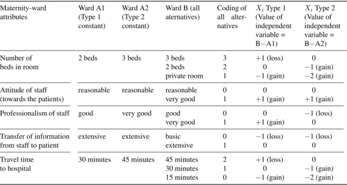
Table 1: Attributes, levels and coding in Type 1 and Type 2 questionnaires Maternity-ward
attributes
Ward A1 (Type 1 constant)
Ward A2 (Type 2 constant)
Ward B (all aternatives)
Coding of all alter-natives
XiType 1
(Value of independent variable = B−A1)
XiType 2
(Value of independent variable = B−A2)
Number of beds in room
2 beds 3 beds 3 beds 2 beds private room
3 2 1
+1 (loss) 0
−1 (gain)
0
−1 (gain) −2 (gain)
Attitude of staff (towards the patients)
reasonable reasonable reasonable very good
0 1
0
+1 (gain)
0
+1 (gain)
Professionalism of staff good very good good very good
0 1
0
+1 (gain)
−1 (loss)
0 Transfer of information
from staff to patient
extensive extensive basic extensive
0 1
−1 (loss)
0
−1 (loss)
0 Travel time
to hospital
30 minutes 45 minutes 45 minutes 30 minutes 15 minutes
2 1 0
+1 (loss)
0
−1 (gain)
0
−1 (gain) −2 (gain)
Note: “Number of beds” was defined by two dummy variables: “3 beds versus 2 beds” and “private room versus 2 beds” in Type 1 regressions; and by “2 beds versus 3 beds” and “private room versus 3 beds” in Type 2 regressions. “Travel time to hospital” included the two dummy variables of “15 minutes versus 30 minutes” and “45 minutes versus 30 minutes” in Type 1 regressions; and “30 minutes versus 45 minutes” and “15 minutes versus 45 minutes” in Type 2 regressions.
cause hospitals are believed to be more diverse in terms of attitude of staff than in terms of professionalism. Diver-sity is prevalent also in terms of information transfer and therefore the two levels are “basic” and “extensive.” The pilot survey and the pilot interviews indicated that unifor-mity simplifies the task of choice between scenarios and that respondents were fully aware of the gap between the two levels that were assigned to each of the attributes.
Travel time has the levels of 15, 30 and 45 minutes to reflect the fact that actual travel time is relatively short because several hospitals are located in the center of the country (the averageactualtravel time of the respondents from residence to the maternity-ward was 19 minutes, with minor differences between the three hospitals: 23, 20 and 16 minutes to each of the hospitals, respectively). A gap of 15 minutes between two successive levels seems therefore reasonable.
A full factorial design that will use all possible combinations of attributes gives rise to 72 scenarios (3*3*2*2*2 = 72; 2 attributes have 3 possible levels each, and each of the other 3 attributes has 2 alternative levels). In order to reduce the number of scenarios to a manage-able size, the SPSS Orthoplan procedure was used to
pro-vide a fractional factorial orthogonal design.3 The
proce-dure’s application gave rise to 16 different scenarios, each representing a hypothetical maternity-ward. If all 16 op-tions were pair-wise compared, a large number of pos-sible discrete choices would emerge. To overcome this difficulty, one scenario was randomly chosen to be con-stant throughout the questionnaire (scenario A1) and each of the remaining 15 scenarios was compared to this cho-sen scenario, concluding in 15 pair-wise combinations. One pair of scenarios had a dominant option (one alterna-tive had superior or identical levels for all attributes) and was used to test for internal consistency.4 Realizing that
it is difficult for women who recently delivered to cope with 15 complex pair-wise choices, the 15 paired combi-nations were split into two subsets. The dominant option was included in each subset, thus giving rise to two ques-tionnaires each with eight choices. The two subsets were randomly distributed among the respondents.
As will be elaborated below, the constant scenario serves as the respondent’s reference point. One of the
3The choice of scenarios that yield an orthogonal design means that
the statistical analysis excludes interactions between attributes.
4A few women (6), who failed the test by preferring the inferior
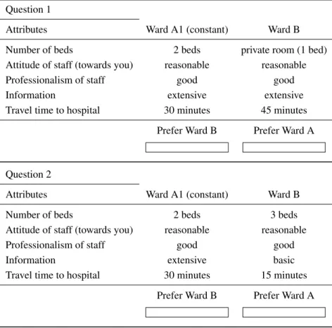
Table 2: Discrete choice questions, Type 1 questionnaire.
You can choose for a delivery, either Ward A1 or Ward B. They differ with respect to a number of attributes. • Assume that all other attributes (on top of the 5 listed ones) are identical in the two wards.
• In each question, Ward A1 is the same and ward B is different. • Which ward would you prefer? (Please tick box below). • Please answer all questions.
Question 1
Attributes Ward A1 (constant) Ward B Number of beds 2 beds private room (1 bed) Attitude of staff (towards you) reasonable reasonable Professionalism of staff good good Information extensive extensive Travel time to hospital 30 minutes 45 minutes
Prefer Ward B Prefer Ward A
Question 2
Attributes Ward A1 (constant) Ward B Number of beds 2 beds 3 beds Attitude of staff (towards you) reasonable reasonable Professionalism of staff good good Information extensive basic Travel time to hospital 30 minutes 15 minutes
Prefer Ward B Prefer Ward A
devices that will be used for the testing of the loss aver-sion theory is a comparison of preference structure that are based on different reference points (constant scenar-ios). For this purpose, we also experimented with an al-ternative constant scenario (A2) that was also randomly chosen from the full set of 16 orthogonal scenarios. Four dominant options were detected within the 15 paired combinations. Three were excluded and one left for the internal consistency test. The remaining pairs of sce-narios were also split into two subsets with six or seven choices, respectively (the dominant option was included in the two subsets) and distributed randomly among the interviewed women. The questionnaires based on each of the two constant wards, are Type 1 and Type 2 question-naires. It follows that all the respondents who received questionnaire Type 1 had the same constant reference set (A1). All the women who answered questionnaire Type 2 also had an identical constant reference set (A2), but the
two sets (A1 and A2) were different. Table 1 presents the two alternative constant scenarios.
Not all attributes changed levels in the two constant hy-pothetical scenarios: The attributes of “attitude” and “in-formation” displayed the same level in A1 and A2, while “professionalism” appeared at the lower level (good) in Questionnaire Type 1 and at the higher level (very good) in Questionnaire Type 2. “Number of beds” and “travel time” was found on the middle level (out of 3 options) in Questionnaire Type 1 and yet on the least desirable level in Questionnaire Type 2. Table 2 contains an example of two of the pair-wise combinations presented to the re-spondents who filled out Questionnaire Type 1.
and one “loss’, whereas in Question 2 the move leads to two “losses” and one “gain.” The respondent is in effect referring to scenario A1 as a reference point while sidering deviations from A1 to B. She therefore must con-sider the gains versus the losses and trade-offs between the attributes when making her quite complex choices. The same applies to interviewees who completed Ques-tionnaire Type 2: they refer to the constant hypothetical scenario A2 as their reference point.
3
The econometric model
Assuming a linear utility function, the marginal change in utility when moving from A5to B is given by
∆UA→B = n
X
i=1
βiXi+u+ε (1)
The observed value of the dependent variable of the estimated preference equation (∆U) is dichotomous and takes the value of 1 if maternity-ward B is chosen and the value of 0 if maternity-ward A is preferred.
The independent variables are theXis, whereXiis the difference in the level of attribute i between B and A. They express changes from the reference level of the con-stant scenario and are outlined in Table 1. Each of the two three-level quantitative attributes was defined using two dummy variables (see note to Table 1).
βi are the parameters of the model that represent marginal utility scores (relative importance) of the at-tributes;uis the error term that represents differences be-tween the various choices of the same respondent (each respondent provides 6–8 discrete choice observations); andεis the error term representing differences between respondents. Interactions between independent variables are not included because anorthogonalfractional design was used.
The data6compiled from the completed questionnaires of the two types were used to estimate two sets of main-effects regressions. To account for the fact that each re-spondent makes several choices, a Random-Effects Probit was used for estimation.7
5The constant hypothetical scenario A is denoted by A1 in
Ques-tionnaire Type 1 and by A2 in QuesQues-tionnaire Type 2.
6Each observation had the value of the dependent variable (either 1
if scenario B was chosen or 0 if A was the preferred scenario) and the deviations between the levels of scenario B and scenario A. See Table 1 for more detail. Each respondent made several choices and therefore contributed several observations.
7Each respondent had an identification number (ID) that was used
for all the responses of this subject (ID=1 for the 6 choices of woman #1; ID=2 for the 6 responses of woman #2 etc.). The statistical Stata program that was used for estimation was “informed” that ID is the subject identifier when applying the random-effects (re) estimation (the Stata command is: re, i (ID), where i refers to the subject ).
4
The loss-aversion hypotheses
A central statement of the loss aversion theory is that utility is reference dependent and that individuals value losses (vis-a-vis the attribute’s reference level), signif-icantly more (in absolute terms) than they value same-sized gains8: e.g., adding one bed to the number of beds in the reference constant scenario (loss) leads to a larger decrease in utility than the increase in utility that is as-sociated with the removal of one bad (gain). The very rich data set, generated by the discrete choice experimen-tal design, is used to test several hypotheses, all derived from the reference-dependence assertion.
Two complementary approaches were employed for testing hypotheses: The first was a comparison of the marginal valuation (utility scores) of positive versus neg-ative same-sized deviations of attributes from the con-stant scenario. Such comparisons can be performed for attributes that exhibit at least three possible levels, with the constant scenario including the middle level. The util-ities of same-sized positive and negative deviations can then be compared. If individuals are loss averse, the disu-tility of negative deviations will be larger than the udisu-tility of positive deviations;
The second approach was the use of two questionnaire types, based on different constant scenarios (A1 and A2): If the respondent was referring to the constant maternity-ward as her reference point, then different constant sce-narios should lead to different estimated utilities for the same attribute. A comparison of the preference structures estimated using data generated by the two questionnaires facilitates statistical testing of loss aversion theory. For instance, assume that a two-level attribute x has different levels in the two alternative constant scenarios: In the first questionnaire it exhibits the less favorable level and in the second it exhibits the more desirable one. It is expected that estimates of the marginal utility score of x based on data generated by the first questionnaire will be smaller than the respective estimates when based on data from the second questionnaire. The justification for this con-clusion rests on the fact that in the first case a deviation represents a “gain” vis-à-vis the reference point whereas in the second case, a deviation represents a “loss.” The DCE is therefore an efficient instrument for soliciting preferences in general and loss aversion components in particular.
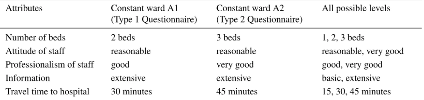
Table 3 illustrates the attribute levels used in the test of loss aversion. For the sake of clarity, the attribute levels of the constant scenarios in the two types of questionnaires (A1 and A1), as well as the definition of all possible at-tribute levels, are repeated. In the Type 1 Questionnaire
8This is the definition proposed by Kahneman and Tversky (1979).
Table 3: Loss aversion hypotheses: levels of the constant scenarios that are used in the two types of questionnaires, as well as all possible attribute levels.
Attributes Constant ward A1 (Type 1 Questionnaire)
Constant ward A2 (Type 2 Questionnaire)
All possible levels
Number of beds 2 beds 3 beds 1, 2, 3 beds
Attitude of staff reasonable reasonable reasonable, very good Professionalism of staff good very good good, very good Information extensive extensive basic, extensive Travel time to hospital 30 minutes 45 minutes 15, 30, 45 minutes
the attributes “number of beds” and “travel time” exhibit the middle level in the constant ward A1, facilitating the following hypotheses that are based on the coefficients of Type 1 regressions (and on the assumption that the degree of diminishing sensitivity/utility is comparable for gains and for losses):
Hypothesis 1: The coefficient of the dummy variable for “3 beds’, that represents a loss, will be significantly larger (in absolute value) than the coefficient of the dummy variable “1 bed” that represents a same-sized gain.
Hypothesis 2: The coefficient of the dummy variable for “travel time of 45 minutes” that relates to a loss, will be significantly larger (in absolute terms) than the coeffi-cient of the “travel time of 15 minutes” dummy variable that relates to the same-sized gain.
Turning to a comparison of regression coefficients based on data generated by the two questionnaires, the following hypotheses can be derived:
Hypothesis 3: The coefficients of “attitude of staff” will not statistically differ by questionnaire type, as in the two questionnaire types they represent the valuation of a gain in attitude.
Hypothesis 4: The coefficients of “information” will not statistically differ by questionnaire type, as in the two questionnaire types they represent the valuation of a loss in information.
Hypothesis 5: The coefficient of “professionalism of staff” will be significantly larger in the regressions based on Type 2 Questionnaires where it relates to the valua-tion of a loss (moving from “very good” to “good’, repre-sented by a difference of−1), whereas in the regressions
based on Type 1 Questionnaires it represents the valua-tion of a gain (moving from “good” to “very good’, rep-resented by a difference of+1).
Hypothesis 6: A larger absolute coefficient for “3 beds” (a loss of one bed compared to the “2 bed” ref-erence level) in the regression based on Type 1 Question-naires will be obtained, in comparison to the coefficient of “two beds” (a same-sized gain vis-à-vis the “3 bed” reference level) in the regression using the Type 2 Ques-tionnaire data.
Hypothesis 7: The coefficient that relates to “travel time of 45 minutes” in Type 1 regression (moving from “30 minutes’ in the reference level to “45 minutes”, that relates to a loss of 15 minutes) is expected to be signif-icantly larger (in absolute terms) than the coefficient of “travel time of 30 minutes” in Type 2 regression (same-sized gain, moving from the reference level of “45 min-utes” to “30 minmin-utes”).
The hypotheses testing will be based on the prefer-ence structure for maternity-ward attributes that were es-timated using the data generated by the two types of ques-tionnaires.
5
Results
Five hundred and forty-two (542) women who had given birth in three large public hospitals located in the Greater Tel-Aviv area in Israel9 comprised the primary study sample. They were surveyed while still in the hospi-tal maternity-wards, by interviewers who provided ex-planations and instructions10. The overall response rate
was about 50% and 542 questionnaires have been fully
9The Rabin medical Center (in Petach Tikva), Sheba (in Ramat-Gan)
and Meir (in Kfar Saba).
10It is recognized in the literature that interviews are the most
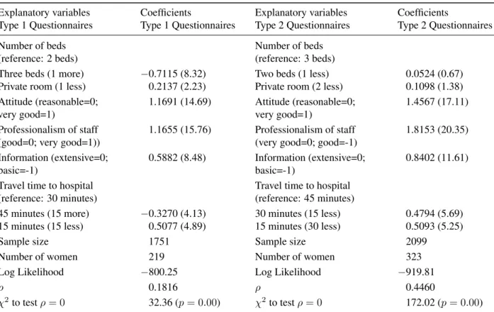
Table 4: Main-effects regressions with two different constant scenarios: Women who gave birth — Israel, 2003. Explanatory variables
Type 1 Questionnaires
Coefficients
Type 1 Questionnaires
Explanatory variables Type 2 Questionnaires
Coefficients
Type 2 Questionnaires Number of beds
(reference: 2 beds)
Number of beds (reference: 3 beds) Three beds (1 more)
Private room (1 less)
−0.7115 (8.32)
0.2137 (2.23)
Two beds (1 less) Private room (2 less)
0.0524 (0.67) 0.1098 (1.38) Attitude (reasonable=0;
very good=1)
1.1691 (14.69) Attitude (reasonable=0; very good=1)
1.4567 (17.11)
Professionalism of staff (good=0; very good=1))
1.1655 (15.76) Professionalism of staff (very good=0; good=-1)
1.8153 (20.35)
Information (extensive=0; basic=-1)
0.5882 (8.48) Information (extensive=0; basic=-1)
0.8402 (11.61)
Travel time to hospital (reference: 30 minutes)
Travel time to hospital (reference: 45 minutes) 45 minutes (15 more)
15 minutes (15 less)
−0.3270 (4.13)
0.5077 (4.89)
30 minutes (15 less) 15 minutes (30 less)
0.4794 (5.69) 0.5093 (5.25)
Sample size 1751 Sample size 2099
Number of women 219 Number of women 323 Log Likelihood −800.25 Log Likelihood −919.81
ρ 0.1816 ρ 0.4460
χ2to testρ= 0 32.36 (p= 0.00) χ2to testρ= 0 172.02 (p= 0.00)
Note: The coefficients of the following pairs of attributes are not significantly different (at a significance level of 0.05): Attitude and Professionalism; Time of 15 minutes more and of 15 minutes less (in absolute values); Infor-mation and Time of 15 minutes less; A private room and Time of 15 minutes more (in absolute value); Three beds and Information (in absolute value).
Note: The coefficients of the following pairs of attributes are not significantly different (at a significance level of 0.05): Two beds and Private room; Time of 15 minutes less and Time of 30 minutes less.
Notes: 1.Zstatistics are in parentheses.
2. Stata 9 was used for estimation (Random-Effect Probit, with no constant).
3. The constant set in Type 1 questionnaires has the following attributes: Number of beds, 2; Attitude, reasonable; Professionalism of staff, good; Information, extensive; Travel time, 30 minutes. The constant set for Type 2 ques-tionnaires has the following attributes: Number of beds, 3; Attitude, reasonable; Professionalism of staff, very good; Information, extensive; Travel time, 45 minutes. The levels of Attitude and Information are therefore the same. Levels of all other attributes are different.
4. The significance of the differences between the main-effects of two groups (not reported) are derived from aχ2test
for equality of coefficients.
completed. Questionnaire Type 1 has been filled out by 219 women (109 and 110 women completed the two sub-versions, respectively), with a total of 1751 observations. Questionnaire Type 2 has been completed by 323 women (161 women completed the first version and 162 the sec-ond one), with 2099 observations.
The age range of the participants in the sample was 18– 47: average age was 31. Four percent were aged over 40. Thirty-one percent of the interviewees were experiencing
their first delivery; the rest, 69%, had had two or more de-liveries.11 Over one quarter (28%) had undergone
high-11Another interesting issue is the effect of experience on preferences.
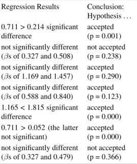
Table 5: Loss aversion hypotheses results: The following table summarizes the relevant regression results and the conclusions of seven hypotheses concerning loss aversion.
Hypotheses Regression Results Conclusion: Hypothesis . . . 1. in Type 1 regression: absolute coefficient of “3 beds” (loss) >
coefficient of “private room” (gain)
0.711 > 0.214 significant difference
accepted (p = 0.001)
2.in Type 1 regression: absolute coefficient of “45 minutes” (loss) > coefficient of “15 minutes” (gain)
not significantly different (βs of 0.327 and 0.508)
not accepted (p = 0.238)
3. coefficient of “attitude” in Type 1 regression (gain) = coefficient of “attitude” in Type 2 regression (gain)
not significantly different (βs of 1.169 and 1.457)
accepted (p = 0.290)
4. coefficient of “information” in Type 1 regression (loss) = coeffi-cient of “information” in Type 2 (loss)
not significantly different (βs of 0.588 and 0.840)
accepted (p = 0.123)
5. coefficient of “professionalism” in Type 1 (gain) < coefficient of “professionalism” in Type 2 (loss)
1.165 < 1.815 significant difference
accepted (p = 0.000)
6.absolute coefficient of “3 beds” in Type 1 (loss) > coefficient of “2 beds” in Type 2 (gain)
0.711 > 0.052 (the latter not significant)
accepted (p = 0.000)
7.absolute coefficient of “45 minutes” in Type 1 (loss of 15 minutes) > coefficient of “30 minutes” in Type 2 (same-sized gain)
not significantly different (βs of 0.327 and 0.479)
not accepted (p = 0.366) The p value is derived from the test for the equality of the respective coefficients.
risk pregnancies. The socio-economic characteristics of the sample were representative of the general Israeli pop-ulation for the relevant age group (see Appendix 1for de-tails).
5.1
Main-effects preference structures
Table 4 presents the main-effects preference structure of maternity-ward attributes.
Before examining if our respondents are loss averse, by testing the seven hypotheses that were formulated above, it is instructive to investigate their preferences for these attributes. However, these two issues are intertwined: if loss aversion is in evidence, then the estimated preference structure will depend on the reference point (constant sce-nario) and data generated by experiments that are based on different reference points, will lead to different prefer-ence equations.
Indeed, Table 4 indicates that the two respective pref-erence structures differ, not only in size of attribute coef-ficients but also in the ranking of attributes’ utility: The most striking difference is related to the room facilities. In Type 2 regressions the two dummy variables that re-late to the number of beds are not significant, indicating that the interviewed women do not gain utility from a de-crease in the number of beds (from 3 beds to 2 beds; p
those who had no experience at all exhibited different preference pat-terns than those with any experience. In the study reported in this paper we excluded the first sub-group and combined the other two that have the same preference pattern.
= 0.50; and even to a private room; p = 0.17). But, in Type 1 regressions a change in the number of beds has a significant effect on utility (or disutility): moving from a two-bed room to a three-bed room results in a signifi-cant drop of 0.711 in utility score (Z = 8.32; p = 0.00), and improving the room conditions from a two-bed room to a private room leads to a significant increase in utility (coefficient of 0.214; Z = 2.23; p = 0.025).
5.2
Testing the loss aversion hypotheses
Table 5 summarizes the tests and conclusions of the seven hypotheses outlined above. The significance of the differ-ence between respective coefficients of the two regression equations (Table 4) are derived from aχ2test for equality
of coefficients.
Discussion of the results follows:
Hypothesis 2: Hypothesis 2 that traveling 15 minutes more (a loss in relation to the reference level of 30 min-utes) is more negatively valued than traveling 15 minutes less (a gain), is not supported. As Type 1 regressions in-dicate, the difference between the coefficients of the two dummy variables in not significant (p = 0.238, for the test of equality of the two coefficients), indicating that the in-terviewed women have a similar valuation of a loss and a same-sized gain.
Hypothesis 3: We find support for Hypothesis 3 that ar-gues that the coefficients of “attitude of staff” are not sig-nificantly different in the two regressions, based on Type 1 and Type 2 Questionnaires (p = 0.290, for the test of equality of coefficients).12. The two coefficients repre-sent a gain compared to the identical reference point in the two questionnaires that is “reasonable attitude” and therefore give an estimate of the marginal utility score of a gain in attitude.
Hypothesis 4: Hypothesis 4 is also supported as the difference between the corresponding coefficients of the “information” attribute in Type 1 and Type 2 regressions is not significant (p = 0.123). In the two questionnaires this attribute is assigned the same level of “extensive in-formation’, indicating that the estimated coefficients re-late to the marginal valuation of a loss of information, from “extensive” to “basic.”
Moreover, combining the two pieces of evidence, namely that the marginal utility score of the “attitude” attribute relates to a gain in attitude, while the marginal utility score of “information” is associated with a loss in information (that is more highly valued than a gain), we can speculate that using the difference between the cor-responding coefficients in order to evaluate the difference in the valuations of “attitude” and “information” is an un-derestimation and gives a lower-limit for the difference. Had “information” also been associated with a gain, we would have arrived at a larger difference, i.e. at the con-clusion that the attribute of “attitude” ranks much higher than the attribute of “information” (with a larger differ-ence than is indicated by our preferdiffer-ence equations).
Hypothesis 5: The coefficient of “professionalism” is indeed significantly larger in Type 1 regression, thus sup-porting Hypothesis 5: there is a positive significant dif-ference of 0.65 (p = 0.000). These results are explained by the fact that in the data of Type 1 questionnaires a gain versus the reference level is in evidence (a change from “good” to “very good”), while is the data of Type 2
12Based on ax2Test for significance between coefficients of two
re-gressions.Not reported in the table.
questionnaires the deviation from the reference scenario is associated with a loss (a change from “very good” to “good”).
Hypothesis 6: The marginal utility score of “3 beds” in responses to Type 1 Questionnaire (absolute value of 0.711) is 14 times (!) larger compared to that of “2 beds” in the responses to the Type 2 Questionnaires (insignif-icant coefficient of 0.052). The former represents a loss compared to the “2 bed” reference level, while the latter manifests a gain versus the “3 bed” reference level. It appears that a gain, in terms of fewer beds in the room, is not appreciated by the women in our sample while a loss (more beds) is painful and highly (negatively) val-ued. This is a very distinct reconfirmation of the asym-metry between gains and same-sized losses.
Hypothesis 7: The difference between a 15-minutes gain in travel time (a decrease from 45 minutes to 30 minutes, Type 2 regression) and a same-sized loss (an increase from 30 to 45, type 1 regression) is not statis-tically significant (p = 0.238). Hypothesis 7 is therefore not supported.
This result is consistent with the rejection of Hypoth-esis 2 and also with the observation that in the Type 2 regression, insignificant differences were found between the valuations of 15 and 30 minutes less travel time, i.e. the two different gains in time have a similar marginal utility score.
To conclude, five of the seven hypotheses have been supported by the regression results, indicating that loss aversion is relevant for the attributes of “professional-ism,” “attitude,” “information” and in particular “num-ber of beds in hospital room.” The rest two hypotheses, which relate to the “travel time” attribute, did not obtain support but have not been reversed either. Could be that travel time is a minor factor within the maternity ward preference structure because the participants had experi-enced only two short episodes of travel (to the maternity ward and back home), leading to neutrality between the (absolute) valuation of a loss and a gain.
6
Summary and discussion
A DCE appears to be a highly suitable tool for loss aversion testing because it estimates the marginal valua-tions of attributes, based ondeviations from a reference point(a constant scenario). Moreover, loss aversion can be tested foreach attribute separatelyrather than for the service as a whole. The DCE method can also be applied to a non-traded service having non-tangible attributes, which implies its flexibility.13
Loss aversion theory was confirmed for four of the five hospital attributes investigated. The results were less con-clusive for “travel time”, probably because traveling is only a short and perhaps marginally meaningful episode for this specific sample population.
The existence of loss aversion also implies that the choice of the constant scenario used in a DCE affects the estimated preference structure obtained: that is, differ-ent constant reference sets result in differdiffer-ent preference structure estimates, if not in changes in the attributes” ranking. It follows that reports of preference structures should include descriptions of the constant reference sce-nario in order to facilitate an accurate description of the coefficients and a distinction between coefficients that present valuations of gains and those that relate to val-uations of losses.
Three unsolved questions merit further study:
The first: what affects the existence and magnitude of loss aversion regarding the various attributes of a com-posite commodity? Is it possible to detect which at-tribute will be subject to a higher level of loss aversion when compared to the others? Our data indicated that “travel time” is not subject to loss-averse preferences and that differences arose in the valuation of a “gain” ver-sus a “loss” between the other four attributes. Further research, involving additional case studies of varied com-posite commodities or services, could lead to greater
gen-13DCEs belong to a set of field experiments that are employed in the
social sciences. Field experiments represent an empirical approach that bridges laboratory data and naturally occurring data (see List, 2006, for a discussion of the methodological contribution of field experiments and a comprehensive overview of the different types of these experiments that are employed in the fields of: Markets; The Economics of Charity; Environmental Economics; Development Economics; and Discrimina-tion). Unlike laboratory experiments, DCEs do not involve any financial incentives for performance and respondents are not paid for answering. While economists presume that experimental subjects do not work for free and they work harder, more persistently, and more effectively, if they earn more money for better performance, the view expressed by most psychologists is that intrinsic motivation is usually high enough to produce steady effort even in the absence of financial rewards; and that while more money may stimulate more effort, the effort does not always improve performance, especially if good performance requires subjects to induce spontaneously a principle of rational choice or judg-ment. However, there is no consensus on this issue and there are studies that have found some effect of real incentives (see Hertwig and Ort-mann, 2001 for a review). Camerer and Hogarth (1999), who reviewed 74 experiments with no, low, or high performance-based incentives, ba-sically found no effect of financial rewards on mean performance (al-though variance is usually reduced by higher payment).
eralization of the results.
A second unresolved question is: What is the role of experience? Economists have claimed that loss aversion will erode as individuals accumulate more experience.14 In most health-care events not much experience can (for-tunately) be accumulated; hence the effect of repeated ob-servations cannot be tested and becomes irrelevant.15
Re-peated experiences can be observed mainly when a pa-tient had a series of treatments or a sequence of health diagnostic tests (e.g. pap smears, blood tests, EKG tests). Experiments conducted among people with chronic con-ditions can therefore be used to examine the effect of ex-perience on the possible erosion of loss aversion.
Third and finally:Are there gender differences in loss aversion? Obviously, our sample, which was composed only of women and pertained to a distinctively feminine scenario — a maternity ward — cannot resolve this is-sue. However, the conduct of a similar study among men could shed some light on this interesting question.
References
Andreoni, J. (1995). Warm-glow versus cold-prickle: The effects of positive and negative framing on cooper-ation in experiments.Quarterly Journal of Economics, 110, 1–21.
Benartzi, S., and Thaler, R. H. (1995). Myopic loss aver-sion and the equity premium puzzle.Quarterly Journal of Economics, 110, 73–92.
Bleichrodt, H., and Pinto J. L., (2002). Loss aversion and scale compatibility in two-attribute trade-offs.Journal of Mathematical Psychology, 46, 315–337.
Bowman, D., Minehart, D., and Rabin, M. (1999). Loss aversion in a consumption/savings model. Journal of Economic Behavior and Organization, 38, 155–178. Bronstein, J., and Morrisey, M. (1991). Bypassing rural
hospitals for obstetrics care. Medical Care, 16, 87– 118.
Brown, S., and Lumley, J. (1994). Satisfaction with care in labor and birth: A survey of 790 Australian women.
Birth,21, 4–13.
Bryan, S., Buxton, M., Sheldon, R., and Grant, A. (1998). Magnetic resonance imaging for the investigation of knee injuries: An investigation of preferences.Health Economics, 7, 595–603.
Cattin, P., and Wittink, D. (1982). Commercial use of conjoint analysis: A survey.Journal of Marketing, 46, 44–53.
14Economists have referred mainly to the experience of selling and
buying experience as reflected in the market place.
15More specifically, women do not have many repeated experiences
Camerer, C. F. (2000). Prospect theory in the wild: Ev-idence from the field. In D. Kahneman, and A. Tver-sky (eds.),Choices, Values and Frames(pp. 288–300). Cambridge, UK: Cambridge University Press. Camerer, C. F., Babcock, L., Loewenstein, G., and
Thaler, R. H. (1997). Labor supply of New York City cabdrivers: One day at a time. Quarterly Journal of Economics, 112, 407–442.
Camerer, C. F., and Hogarth, R. M. (1999). The effects of financial incentives in experiments: A review of capital-labor production framework. Journal of Risk and Uncertainty, 19, 7–42.
Genesove, D., and Mayer, C. (2001). Loss aversion and seller behavior: Evidence from the housing market.
Quarterly Journal of Economics, 116, 1233–1260. Green, P., Carmon, F., and Wind, I. (1972). Subjective
evaluation models and conjoint measurement. Behav-ioral Science, 7, 288–299.
Hardie, B. G. S., Johnson, E. J., and Fader, P. S. (1993). Modeling loss aversion and reference dependence ef-fects on brand choice. Marketing Science, 12, 378– 394.
Hartman, R. S., Doane, M. J., and Woo, C. K. (1991). Consumer rationality and the status quo. Quarterly Journal of Economics, 106, 141–162.
Hertwig, R., and Ortmann, A. (2001). Experimental prac-tices in Economics: A methodological challenge for Psychologists? Behavioral and Brain Sciences, 24, 383–451.
Janssen, P. A., Klein, M. C., Harris, S. J., Soolsma, J., and Seymour, L. C. (2000). Single room maternity care and client satisfaction.Birth, 27, 235–243.
Jullien, B., and Salanie, B. (2000). Estimating prefer-ences under risk: The case of racetrack bettors. Jour-nal of Political Economy, 108, 503–530.
Kahneman, D., and Tversky, A. (1979). Prospect theory: An analysis of decision under risk. Econometrica, 47,
263–291.
Kobberling, V., and Wakker P. P. (2005). An index of loss aversion.Journal of Economic Theory, 122, 119–131. Koszegi, B., and Rabin, M. (2006). A model of reference-dependent preferences. Quarterly Journal of Eco-nomics,121, 1133–1165.
List, J. A. (2006). Field experiments: A bridge between lab and naturally occurring data. Advances in Eco-nomic Analysis and Policy,6, Article 8, 1–45 (Berke-ley Electronic Press).
Luce, D., and Tukey, J. (1964). Simultaneous conjoint measurement: A new type of fundamental measure-ment.Journal of Mathematical Psychology,1, 1–27. McGuirk, M. A., and Porell F. W. (1984). Spatial
pat-terns of hospital utilization: The impact of distance and time.Inquiry, 21, 84–95.
Myagkov, M., and Plott, C. R. (1998). Exchange economies and loss exposure: Experiments exploring prospect theory and competitive equilibria in market environments. American Economic Review,87, 801– 828.
Neuman E., and Neuman S. (2007). Explorations of the effect of experience on preferences for a health-care service. Discussion Paper No. 6608, CEPR, London. Opaluch, J., Swallow, S., Weaver T., Wessells, C., and
Wichelns, D. (1993). Evaluating impacts from nox-ious facilities: Including public preferences in current sitting mechanisms. Journal of Environmental Eco-nomics and Management, 24, 41–59.
Phibbs, C., Mark, D., Luft, H., Petzman-Rennie, D., Garnick, D., Lichtenberg, E., and McPhee, S. (1993). Choice of hospital for delivery: A comparison of high risk and low risk women. Health Services Research, 28, 201–220.
Rahtz, D. R., and Moore, D. L. (1988). An examination of attribute saliency in the obstetrics/gynecology profit center.Journal of Health Care Marketing, 8, 50–53. Robinson, A., Loomes, G., and Jones-Lee, M. (2001).
Visual analogue scales, standard gambles and relative risk aversion.Medical Decision Making,21, 17–27. Ryan, M., and Hughes, J. (1997). Using conjoint
analy-sis to assess women’s preferences for miscarriage man-agement.Health Economics, 6, 261–273.
Ryan, M., McIntosh, E., and Shackley, P. (1998a). Using conjoint analysis to elicit the views of health service users: An application to the patient health card.Health Expectation, 1, 117–129.
Ryan, M., McIntosh, E., and Shackley, P. (1998b). Methodological issues in the application of conjoint analysis in health care.Health Economics, 7, 373–378. Sadler, L. C., Davison, T., and McCowan, L. M. E. (2001). Maternal satisfaction with active management of labor: A randomized controlled trial. Birth, 28, 225–235.
Salkeld, G., Ryan, M., and Short, L. (2000). The veil of experience: Do consumers prefer what they know best?.Health Economics, 9, 267–270.
San Miguel, F., Ryan, M., and Scott, A. (2002). Are pref-erences stable? The case of health care. Journal of Economic Behavior and Organization, 48, 1–14. Scott, A. (2002). Identifying and analysing dominant
preferences in discrete choice experiments: An appli-cation in health care.Journal of Economic Psychology, 23, 383–398.
Shalev, J. (2000). Loss aversion equilibrium. Interna-tional Journal of Game Theory,29, 269–287.
Tversky, A., and Kahneman, D. (1991). Loss aversion in risk-less choice: A reference dependent model. Quar-terly Journal of Economics, 106, 1039–1061.
van Osch, S. M. C., Wakker, P. P., van den Hout, W. B., and Stiggelbout, A. M. (2004). Correcting biases in gamble and tradeoff utilities. Medical Decision Mak-ing,24, 511–517.
van Osch, S. M. C., van den Hout, W. B., and Stiggel-bout, A. M. (2006). Exploring the reference point in prospect theory: Gambles for length of life. Medical Decision Making, 26, 338–346.
Vick, S., and Scott, A. (1998). Agency in health care: Examining patients preferences for attributes of the doctor-patient relationship. Journal of Health Eco-nomics, 17, 587–605.
Wardman, M. (1988). A comparison of revealed prefer-ence and stated preferprefer-ence models. Journal of Trans-port Economics and Policy,22, 71–91.
Wakker, P., and Tversky, A. (1993). An axiomatization of cumulative prospect theory.Journal of Risk and Un-certainty,7, 147–176.
Wilcock, A., Kobayashi, L., and Murray, I. (1997). Twenty-five years of obstetric patient satisfaction in North America: A review of the literature. Journal of Prenatal and Neonatal Nursing,10, 36–47.
Appendix 1: Socio-economic
charac-teristics of the sample
The socio-economic background of the respondents is representative of the Israeli general population in this age group (18 — 47).
The average age is 30.65 (10% were aged below 25 and 4% above 40).
The ethnic composition of the sample resembled the ethnic stratification in the Israeli population: 26% were born in Asian/African countries (referred to as Easterners or Mizrachim); 33% were born in European or English-speaking countries (referred to as Westerners or Ashke-nazim); and the remaining 41% were native Israelis. The women were highly educated, with almost half (46%) having earned an academic degree; only 4 (less than 1%) out of 542 women had not studied beyond elementary school. The questionnaire also included questions on per-sonal and household income. As all women were on ma-ternity leave, many declared themselves as not working. As to household income: 36% reported above average; 56%, average; and 8%, below average.
The respondents were also asked to relate to their reli-gious affiliation: About half said they were secular, one quarter traditional and one quarter observant or ultra reli-gious.