Wealth composition, endogenous fertility and the dynamics of income inequality

Wealth Composition,

Endogenous Fertility and

the Dynamics of Income Inequality

Fernando A. Veloso· Department ofEconomics

Ibmec November 14,2002

Abstract

This paper analyzes how differences in the composition of wealth between human and physical capital among families affect fertility choices. These in tum influence the dynamics of wealth and income inequality across generations through a tradeoffbetween quantity and quality of children. Wealth composition affects fertility because physical capital has only a wealth effect on number of children, whereas human capital increases the time cost of child-rearing in addition

to the wealth effect. I construct a model combining endogenous fertility with borrowing constraints in human capital investments, in which weaIth composition is determined endogenously. The model is calibrated to the PNAD, a Brazilian household survey, and the main findings of the paper can be summarized as follows. First, the model implies that the cross-section relationship between fertility and wealth typically displays a U-shaped pattem, reflecting differences in wealth composition between poor and rich families. Also, the quantity-quality tradeoff implies a concave cross-section relationship between investments per child and wealth. Second, as the economy develops and families overcome their bOlTowing constraints, the negative effect of weaIth on fertility becomes smaller, and persistence of inequality declines accordingly. The empirical evidence presented in this paper is consistent with both implications .

1.lntroduction

This paper analyzes the implications of the interaction between wealth composition,

fertility and investments in children for the dynamic behavior of the income distribution among

families. Wealth composition affects fertility because physical capital has only a wealth effect on

the optimal number of children, whereas human capital increases the time cost of child-rearing in

addition to the wealth effect. Fertility choices in turn influence the dynamics of income inequality across generations due to a tradeoff between quantity and quality of children.

Several studies suggest that human and physical capital have different qualitative effects

on fertility and investments in children. Becker and Barro (1988), Benhabib and Nishimura

(1993) and Alvarez (1999) analyze fertility models in which families are heterogeneous in their

physical capital stocks. In these models, rich families dilute their wealth by having more children

than poor families, and fertility behavior leads to long-run equality among families.

Becker, Murphy and Tamura (1990), Tamura (1994) and Palivos (1995) study the role of

heterogeneity in human capital in generating differences in fertility and investment decisions

among families. Since child-rearing requires parental time, human capital increases the

opportunity cost of children, and fertility is negatively related to income. Because of the tradeoff

between quantity and quality of children, endogenous fertility leads to long-run income

inequality .

The main contribution of this paper is to analyze a model of fertility and investment

decisions in which the wealth and income composition are determined endogenously fiom the

allocation of investments in children between human and physical capital. The endogeneity of

wealth composition allows for a characterization of the conditions under which fertility is an

equalizing force, and when it creates inequality.

Recent papers by Dahan and Tsiddon (1998), Knowles (1999), Kremer and Chen (2000),

Doepke (2002) and Greenwood, Guner and Knowles (2002) also analyze the effects of

differential fertility on the dynamic behavior of the income distribution, but they do not consider

effects of the composition of wealth on income distribution, but they do not model fertility

decisions. Lucas (2002) presents a representative agent model of endogenous fertility with

human and physical capital, but its implications for income inequality are not analyzed.

In order to analyze the interaction between wealth composition, fertility and the dynamics

of inequality, I combine a borrowing-constraints model of human and physical capital

investments with a model of fertility behavior.

I assume that families may invest in children's human and physical capital, but c~ot

borrow to finance their human capital investments. In any period, families are divided into two

groups. Richer families typically are unconstrained, and make efficient human capital

investments. Additional investments are made in the form of physical capital. Since the children

of unconstrained families are also unconstrained, this group tends to have the same leveI of

(efficient) human capital, and different physical capital stocks.

Poorer families are typically constrained, and make investments in children only in the

form of human capital. If the children of poor families are also constrained, they will have the

same stock of physical capital, equal to zero, and will be heterogeneous in their human capital

stocks.

Since the source of wealth variations differs for constrained and unconstrained families,

their fertility behavior differs as well. In particular, the negative effect of wealth on fertility is

larger for constrained than for unconstrained families, and the cross-section fertility-wealth

profile typically displays a U-shaped pattem at any point in time. Because of the tradeoff

between quantity and quality of children, this implies a concave cross-section relationship

between investments per child and parental wealth.

The model is calibrated to data from the 1996 Pesquisa Nacional de Amostra Domiciliar

(PNAD), a Brazilian household survey. The PNAD is a series of annual representative

cross-sections of the Brazilian population collected by the Instituto Brasileiro de Geografia e

in general, and Brazil in particular, are typicallycharacterized by significant cross-section

variation in fertility across education and income classes. I

The numerical simulations suggest three qualitatively different long-run pattems of

wealth and income distribution. First, if the degree of intergenerational altruism, the time cost of

children and the productivity of human capital investments are high relative to the fertility

preference parameter, all families eventually overcome their borrowing constraints and there is

long-run income equality. The negative effect of wealth on fertility declines across generations,

which reduces persistence of inequality.

Another pattem generated by the model is one in which the degree of altruisp:l, the time

cost of children and the productivity of human capital investments are not high enough relative

to preferences for numbers of children to allow families to overcome their borrowing constraints,

but are large enough to generate convergence among borrowing-constrained dynasties.

The third possible outcome is a situation in which the degree of altruism, the time cost of

children and the productivity of human capital investments are too low relativ~ to preferences for

numbers of children, so that numbers of children are sufficiently high to generate long-run

inequality.

I provide empirical evidence on the main implications of the model based on an empirical

analysis of the PNAD and results from other studies. The evidence shows that the

fertility-income cross-section profile typically displays a U-shaped pattem, consistent with the model.

The interaction between quantity and quality of children tends in tum to generate a concave

investment-income cross-section profile for the PNAD data, even though the evidence is mixed

for other studies.

I also explore the implications of the model regarding the dynamic behavior of the degree

of intergenerational persistence of inequality. The simulations suggest that, given the calibrated

parameters, the negative effect of wealth on fertility tends to become smaller across generations,

reflecting a weaker cross-section association between wealth and labor income over time.

Moreover, the quantity-quality tradeoff will tend to reduce the degree of persistence in inequality

over time.

In order to verify this implication of the model, I compare the degrees of persistence in

wages and the coefficients obtained from a regression of fertility on wages for Brazil and the

United States. The results suggest that a larger negative effect of wages on fertility increases the

persistence of inequality in Brazi!.

This paper is organized as follows. Section 2 presents the mode!. Section 3 calibrates the

mode! to the 1996 PNAD, and illustrates the possible outcomes with the aid of simulations.

Section 4 presents empirical evidence supporting the implications of the mode!. Section 5

concludes and provides directions for future research.

2. TheModel

Consider an economy inhabited by M dynasties, indexed by i

=

I, ... , M . Each dynasty is defined by a parent and her descendants. Each person lives for two periods: childhood and

adulthood. Parental variables are indexed by t, while children variables are indexed by t + 1 .

Families have two sources of wealth: human capital, h, and physical capital, k .

First-generation parents are heterogeneous in their stocks of human and physical capital,

{ h,/ ,

kOi}_

. Parents are assumed to have identical preferences over their consumption, c"

.-I, ... ,M

number of children, n" and utility per child, Ut+I' described by

U,

=

a logc,

+

ylogn,

+

f3u'+1

where

a

> O, Y > O and O < f3 < 1 .

Parents are endowed with one unit of time, and spend íl units of time per child and if> units of the consumption good rearing their children. Hence, parents work 1-íln, units of time,

earning a wage rate w" described by the following functional specification:3

where A > O and O <

e

< 1.

I will assume that the rental price of capital is detenruned exogenously, at the constant

leveI r. Parents choose investments in each child's human capital, h'+I' and physical capital, k'+I' but they cannot borrow against their children's eamings in order to finance human capital investments.

The recursive fonnulation ofthe decision problem of a typical parent can be described as

v(h,k)= m~,{alogc+ ylogn+ f3v( h',k')} c,n,h,k

s.t.

k'

~O 1

O<n<-_{- - íl}

c+n(if>+h' +k')

=

(l-íln) Ahl

-e +(I+r)k

where h' and k' denote human and physical capital per child, respectively.

(1)

The budget constraint captures the interaction between the quantity and quality of

children through the tenn n, (ht+1 + kt+1 ). Borrowing constraints are captured by the restriction

It is convenient to rewrite (I) in tenns of full-time wealth, y == Ahl

-e

+(1 + r) k, and

fulI-time labor income, yL == Ahl-e :

3 See Loury (1981), Becker and Tomes (1986) and Mulligan and Song Han (2000) for similar specifications ofthe

v(h,k)==

m3;X,{alogc+ ylogn+

.Bv(h',k')}

c,n.h.k

I O<n<-_{- - À}

c+n (ifJ+h' +k' +ÀAhl-e) == Ahl-e +(l+r) k

(2)

The fonnulation in (2) makes explicit the fact that human capital affects the price of children through the tenn ÀAhl-e, while physical capital has only a wealth effect on number of

children. This asymmetry between human and physical capital, combined with the interaction between number of children and investments in the budget constraint, is crucial in generating a link between wealth composition and investments per child.

The Euler equation for unconstrained families, that is, families making positive physical capital investments per child, k'+1 > O , is given by

C'+I

==.B

(l+r)

(3) c, n,

The Euler equation for constrained families, that is, families for which optimal physical capital investments in the absence of constraints satisfy kt+1 < O, is given by

(4)

c, n,

Notice that the rate of return on investments for both constrained and unconstrained families depend on the optimal fertility rate, n,. Unconstrained families equalize the rate of retum between human and physical capital investments, which implies:

1

h ==[A(l-e){I-Àn,+I)J

Since the fertility rate of the next generation affects the amount of time they alIocate to

the marketplace, optimal human capital investments, h'+l' depend on n'+l' as shown in (5). This dependence of current investments on the fertility behavior of future generations makes it very

difficult to characterize the model analytically, and makes it necessary to compute numerical

simulations to understand the behavior of the mode!. 4

3. Model Simulations

3.1. Calibration

The baseline parameters will be calibrated to data from the 1996 Pesquisa Nacional de

Amostra Domiciliar (PNAD), a Brazilian household survey. The PNAD is a series of

representative cross-sections of the Brazilian population which have been colIected annualIy

(except for 1980, 1990, 1991 and 2000) since 1973 by the Instituto Brasileiro de Geografia e

Estatística (IBGE). 5

I assume that a generation takes 25 years. The annual rate of return on physical capital is

chosen to match the average rate of return on 30-year V.S. govemment bonds, which is about

5.7%. This implies that the net rate of return on physical capital over a generation, r, is chosen

to be r = 3. These numbers were taken from Mulligan and Song Han (2000).

I require that

f3

(1

+ r )

=

I , under the assumption that r corresponds to the steady state

rate of return for the V.S.6 Hence

f3

=

0.25, which corresponds to an annual altruism rate of 0.946.

4 Kremer and Chen (2000) were faced with the same difficulty, and they dealt with it by assuming that market wages

depend on the size ofthe labor force, rather than the amount ofman-hours employed in production.

5 The PNAD is close to a nationally representative sample, though it is not fully representative of rural areas,

especiaJly in the remote frontier regions.

6 Laitner (1992) and Navarro-Zermeno (1993) suggest that consumption does not grow across generations among

The elasticity of wages with respect to hwnan capital is 1-

e.

If we take a log-linear approximation to the frrst-order condition for hwnan capital investrnents in children, we obtain the following equation:

(6)

À-L

where Y L is the sample average of the share of time costs in total fertility costs and cons

I/>+Ày

denotes a constant.

I was not able to compute this share from the Brazilian data, so I used the share of time costs for American women with only elementary education, obtained from Espenshade (1977). This implies a share offifty-percent. Since the average woman in the sample used to estimate (6) had on average four years of schooling, this may provide a reasonable approximation for Brazil. I then estimated (6) using years of schooling of the mother and the oldest aduIt child, and obtained a coefficient on log h, equal to 0.4. This implies that 1-

e

=

0.8, so I set the base1ine value of

e

to 0.2.7

In order to provide an estimate of the fraction of time alIocated to child-rearing, À, I use the restriction imposed by the modeI on the maximwn ferti1ity rate:

where n_max is the maximwn nwnber of children and the total time endowment is normalized to 1. This restriction has to be satisfied in order for the head of household to supply positive labor hours.

I computed n_max by choosing the highest nwnber of children currently alive for married women aged 40-60 currently employed, and then used the restriction above to estimate À. I

considered only women because there is considerable evidence that women allocate a higher

fraction of their time to child-rearing than men.8 I used number of children currently alive as a

measure of fertility, rather than number of children-ever-bom, to reduce the effect of child

mortality on the empirical measure of fertility. The chosen age bracket for married women was

chosen in order to obtain a measure of completed fertility. For this sample, n_max was found to

equal 7, which implies Â, =0.14.

I order to estimate the parameter A in the wage function, I used the estimated values of

e,

Â, and

r

and the expression for the optimal human capital per child given by (5). To compute

the optimal human capital investment per child, I computed the average schooling among

children aged 14-21 still living with their parents. Moreover, this measure was calculated for

parents in the highest income decile, because they are more likely to be making oprimal human

capital investments in children. The restriction that children live with their parents is necessary

for one to be able to link data on parents and their children. I also assumed that these families are

in steady state, so that nt+1

=

n,. These calculations lead to an estimate of A equal to 5.

In order to estimate the preference parameters

a

and

r,

I assume that

a

+

y

=

1, and use

the fact that a and y are the shares of parental consumption and total expenditures in children

on family income, respectively. These shares were obtained from the 1987/88 Pesquisa de

Orçamento Familiar (POF), a Brazilian household survey that provides detailed data on family

expenditures for 9 metropolitan regions. The POF data set implies a share of total expenditures in

children of approximately one third, which implies that

a

= 0.67 and

r

= 0.33.9

I estimated the goods cost offertility per child,

l/J,

by using

Â,Y~L

=

0.5, the estimated

l/J+Â,y

value of Â, and the average value of labor income (computed in model units, see below), which

yields

l/J

=

0.5.10

I also chose the range and the initial distribution of the state variables, human and

physical capital, in order to match the corresponding values for the PNAD 96. In particular, the

8 See Leibowitz (1974).

9 Espenshade (1984) estimates that expenditures on children account for between 30 and 50 percent oftotal family

expenditures in the V.S.

initial distribution consists of 10 pairs of human and physical capital combinations, chosen to fit

the distribution of schooling and fmancial wealth across income deciles among married couples

with women aged 40-60 in 1996.

These human-physical capital initial pairs were constructed as follows. I used the wife's

average schooling by deciles as a measure of the distribution of human capital among families. 11

I then used the wage function of the model, calibrated as described above, to compute the

lifetime labor income of the household head. From the PNAD 96, I computed the average ratio

between capital income (interest, dividends and rent) and labor income for each decile. Finally, I

applied these ratios to the constructed measures of lifetime labor income, and used the calibrated

interest rate, r, to construct measures of the capital stock for each decile. The resulting pairs of

human and physical capital were used to compute alI time series simulated from the model.

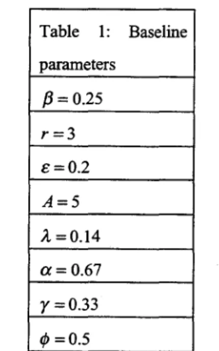
Table 1 presents the baseline parameter values. They will be used in alI simulations,

unless noted otherwise.

3.2. Simulations

In this subsection, I will simulate the model presented in section 2 for three different

parameterizations, intended to illustrate the different long-run pattems that may arise. In section

4, I will estimate the empírical counterparts to the simulations and will assess to what extent the

model is able to match the Brazilian data.

One possibility is that the degree of altruism, the time cost of children and the

productivity of human capital investments are not high enough relative to preferences for

numbers of children, but are large enough to generate convergence among

borrowing-constrained families. This possibility wilI be analyzed in the first simulation.

11 Since husbands' and wives' education are highly correlated, the results are similar when we use the former as a

A second possibility corresponds to the case in which all families eventually overcome

their borrowing constraints and there is long-run wealth and income equality among familieso

This possibility will be analyzed in the second simulationo

A third possibility is that the degree of altruism, the time cost of children and the

productivity of human capital investments are toa low relative to preferences for numbers of

children, so that the number of children is sufficiently high to generate long-run inequalityo This

possibility will be considered in the third simulationo

a) Baseline case

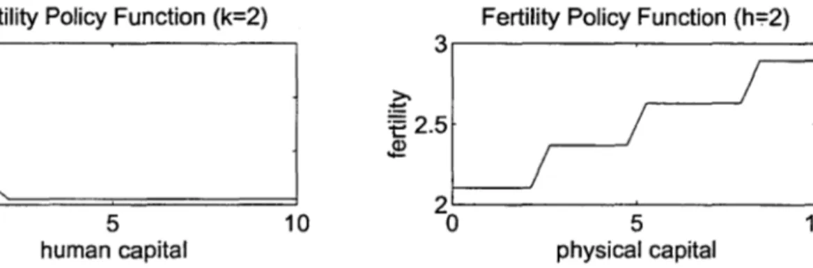
Figures 1 and 2 present simulation results for the baseline parameterizationo Figure 1

displays the policy function for fertility as a function of the state variables, human and physical

capital o The policy funotion for fertility shows that fertility decreases with human capital, and

increases with physical capital. This asymmetry of fertility behavior with respect to the source of

wealth is particularly pronounced at low human and physical capitallevelso

The policy function for physical capital investments for this parameter configuration is

trivial, since all families are borrowing-constrained and thus do not leave any bequests in the

forro of physical capital. This is consistent with the 1996 PNAD data for Brazil, which shows

that for a large majority ofthe population the share of asset income in total income is very smallo

The first step in the analysis is to study how the cross-section relationship between

fertility and parental wealth affects the cross-section investment profile through the

quantity-quality tradeoff, and how both cross-section relationships are affected by the cross-section

correlation between parental wealth and labor incomeo All simulated cross-section relationships

were obtained by simulating (2) using the baseline parameter values (unless noted otherwise) and

the initial distribution of pairs of human and physical capital, {hOi, kOi ,i = 1 '000'

N},

constructed in

the way described in the previous subsectiono

The three plots in Figure 2 illustrate the relationships between wealth composition,

Ah,-e

generation. The labor income-share, l-e t , increases slightly at low-wealth leveIs,

Ah,

+ (1+

r )k,

Ah/-e

+

(1

+

r)

k, , and declines for higher leveIs of wealth. Fertility,

n"

declines at low leveIs of

wealth, then becomes constant, and increases slightly at the highest end of the wealth

distribution.

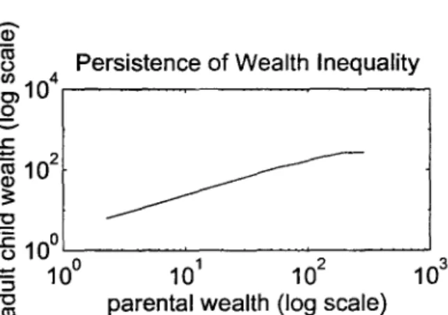
The reduction in fertility among poor and middle-income families tends to increase

persistence of inequality, as captured by the slope of the graph that relates aduIt child's wealth,

Ah,+/-e

+ (1+

r

)k,+" to parental wealth, Ah/-e

+(1 +

r)

k,. Further increases in parental wealth

are associated with constant and rising fertility, which reduces persistence of inequality among

richer families.

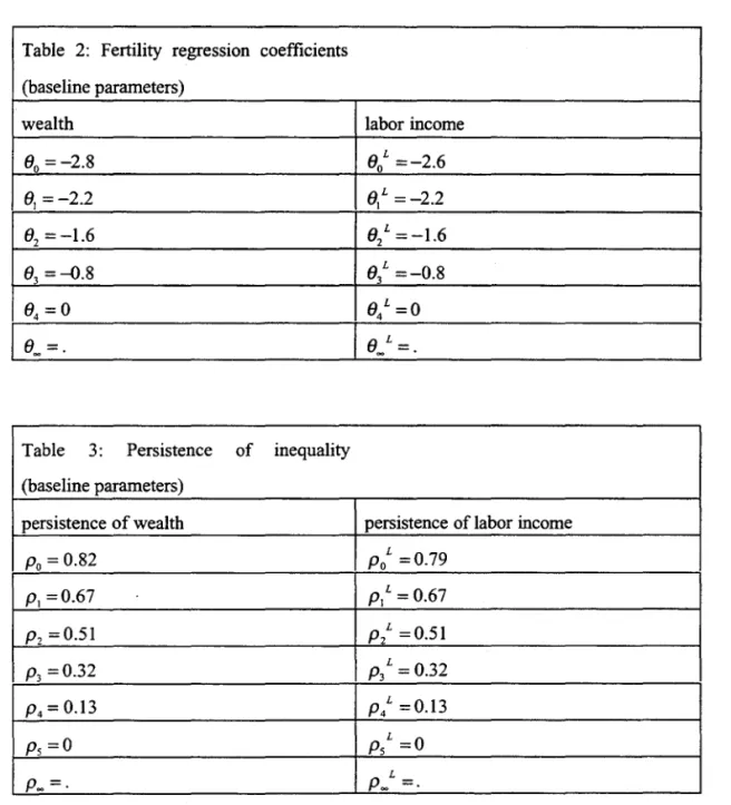
Table 2 displays the dynamic behavior of the fertility-wealth (labor income) relationship.

These estimates, denoted by 0, and O,L, respectively, are ordinary least-squares coefficients obtained by regressing fertility, n" on parentallog wealth (labor income), log y, (log y,

L) ,

where

the observations were generated by simulating time series of wealth and labor income for all

families.

Table 2 shows that the negative effect of wealth (labor income) on fertility in the

cross-section of families declines across generations. At t =4, all families have the same fertility rate

(0₄

=

O), and in the long-run the fertility regression coefficient cannot be calculated, since there is long-run equality (0_ =.).

Table 3 displays the dynamic behavior of the degrees of intergenerational persistence of

inequality of wealth and labor income, denoted p, and p,L, respectively. These estimates are ordinary least-squares coefficients obtained by regressing total aduIt child's log wealth (labor

income), 10gy,+,(logy,+,L) , on parentallog wealth (labor income), logy,(logy/), where the

observations were generated by simulating time series of wealth and labor income for all

families.12

Three features of Table 3 deserve comment. First, both degrees of persistence of

inequality are always less than one, which implies convergence. Second, both persistence

coefficients decline monotonically over time. Third, the decline in persistence of inequality is

very slow. In fact, as can be observed from Table 3, only at t = 5 persistence is zero for both

wealth and labor income, implying convergence after six generations.

The baseline parameterization leads to policy functions and time series that resemble the

equilibrium family behavior in Becker, Murphy and Tamura (1990). Families derive all their

income from labor, and fertility is negatively related to income, at least at low-income leveis.

The dynamic behavior of income distribution for the baseline parameterization differs from the

one implied by Becker, Murphy and Tamura (1990), however, in two important aspects. First,

the human capital technology in the model presented in this paper is concave. Second, because of

the concavity assumption, the model tends to generate long-run equality in labor shares across

families, which in turn tends to reduce the negative correlation between fertility and parental

wealth, which reinforces the undedying tendency for long-run equality.

b) Increase in time spent in child-rearing

(À

=

0.4)

Figures 3 and 4 present simulation results for the case in which À

=

0.4 (as opposed to

À

=

0.14 in the baseline case). The parameter À is the fraction of time devoted to child-rearing.

An increase in À may be interpreted as a reduction in the productivity of child-rearing or,

conversely, as an increase in the cost of fertility. All other parameters and the initial distribution

of state variables remain the same.

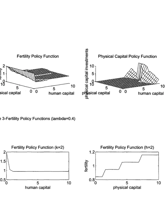
Figure 3 displays the policy functions for fertility and physical capital investments,

respectively, as functions of the state variables, human and physical capital. As observed in the

previous example, for any given leveI of physical capital, fertility declines when human capital

increases. AIso, for any given leveI of human capital, fertility increases with physical capital.

One interesting feature of Figure 3 is that, as opposed to the baseline case, a significant

many families leave positive bequests to their children in the fonn of physical capital. This result illustrates the fact that the extent to which borrowing constraints are binding may be significantly affected by fertility decisions, since the only difference between the policy functions displayed in Figures 1 (baseline case) and 3 is that the latter are computed for a higher À. .

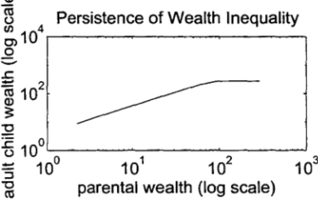
The three plots in Figure 4 illustrate the relationship between wealth composition, fertility behavior, and investments per child at t

=

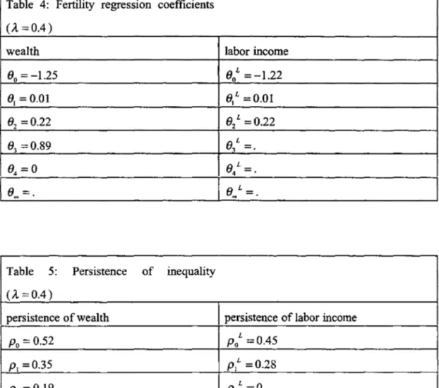
O. The cross-section relationship between fertility and parental wealth displays a U-shaped pattem, which mirrors the inverse U-shaped relationship between labor share and parental wealth.13 The positive relationship between number of children and parental wealth at higher leveIs of wealth contributes significantly for the very low degree of persistence in wealth inequality among rich families.

Table 4 shows that the effect of wealth (labor income) on fertility in the cross-section of families becomes positive at t

=

1. At t = 4, all families have the same fertility rate (84

=

O), and

in the long-run the fert.lity regression coefficient cannot be calculated, since there is long-run equality ( 8 ~

= . ).

Table 5 displays the dynamic behavior of the degrees of intergenerational persistence of inequality of wealth and labor income. From t

=

5 on, there is wealth and income equality among families. The degree of persistence of labor income declines monotonically, as families overcome their borrowing constraints across generations. At t = 2 all families are unconstrained, and this is reflected in a persistence coefficient for labor income equal to zero. There is still some persistence in wealth, however, as parents make investments in children in the fonn of physical capital. At t

=

3, all families have the same efficient human capital leveIs, and this leads to equality oftotal investments in children, as in Becker and Barro (1988).

The case in which À. = 0.4 leads to a dynamic behavior that combines elements from Becker and Barro (1988) and Becker, Murphy and Tamura (1990). lnitially, most farnilies derive all their income from labor, and fertility is negatively related to income at low-income leveIs. At high-income leveIs, fertility is positively related to income, as these families derive most of their

13 See Becker and Tomes (1976) for a theoretical analysis that also generates a U-shaped fertility-income

income from physical capital. As the economy develops, constrained families eventually become

unconstrained, and the relationship between labor share and wealth becomes negative. Because

of the change in the cross-section wealth composition, the relationship between fertility and

wealth becomes positive, which leads to equality in investments across families through the

quantity-quality tradeoff.

c) Reduction in the rate of return to human capital

(e

=

0.5).

Figures 5 and 6 present simulation results for the case in which

e

=

0.5 (as opposed to

e

=

0.2 in the baseline case). The parameter

e

affects the rate of return of human capital

investments. It can be interpreted as a technological parameter, or as capturing the effect of institutions and govemment policy on the efficiency of investments in education.14 All other

parameters and the initial distribution of state variables remain the same.

Figure 5 displays the policy function for fertility. For any given levei of physical capital,

fertility declines when human capital increases. For any given leveI of human capital, fertility

increases with physical capital. This asymmetry of fertility behavior with respect to the source of

wealth is qualitatively similar to the one observed for the higher productivity case (Figure 1), but

is considerably sharper.

The policy function for physical capital investments for this parameter configuration is

trivial, since alI families are borrowing-constrained and thus do not leave any bequests in the

form of physical capital.

The three plots in Figure 6 illustrate the relationship between wealth composition,

fertility behavior, and investments per child at t

=

O. The qualitative patterns are similar to the

ones observed for the higher rate of return case (Figure 2). The main difference is that total

investments in children are smaller when

e

=

0.5 . It should also be noted that, despite the lower

productivity, fertility leveIs at t

=

O are higher than the ones ohserved for

e

=

0.2 .

14 HaII and Jones (1999) interpret productivity parameters as functions of the economic infrastructure, including

Table 6 shows that the negative effect of wealth (labor income) on fertility persists for several generations. If we compare Table 6 to Table 2, we can observe that the negative effect of wealth on fertility is larger in every period when the rate of return is smaller.

Table 7 displays the dynamic behavior of the degrees of intergenerational persistence of inequality of wealth and labor income. The dynamic partem of the coefficients is considerably different from the one displayed when the rate of return of human capital investments is higher (Table 2). When the rate of return is low, both degrees of persistence increase over time, and from t

=

4 on the relative distance in wealth and labor income among dynasties remains constant (degree of persistence equals 1). If we compare Table 7 to Table 2, we can observe that persistence of inequality is higher in every period when the rate of return is smaller, which is consistent with the fertility pattem displayed in Table 6.

This exerci se suggests that persistence of inequality is affected not only by the differences in fertility rates across income classes, but also by fertility leveIs. Long-run inequality in this example thus arises because of endogenous fertility decisions and, particularly, by the fact that poor families tend to have a number of children excessively high relative to the leveI of technology.

4. Empirical Evidence

4.1. Evidence on U-shaped fertility-income cross-section profile.

The interaction between quantity and quality of children tends in turn to generate a

concave quality-income cross-section profile, where quality is captured by either schooling or

income of the aduIt child.

Table 8 presents ordinary least-squares (OLS) regressions of fertility, adult child's

schooling and adult child's log income on parental log income and log income squared, using

data from the 1996 PNAD.15 Parental and adult child's family income are used as proxies for

parental and child's wealth. 16 I also tried to fit polynomials of higher order to the data, but onIy

the coefficients on father's log income and log income squared were found to be statistically

significant. 17

Table 8 shows that the coefficient on log parental income in the fertility regression is

negative, while the coefficient on log income squared is positive. AIl coefficients are significant

at the one-percent leveI. The estimated fertility-income profile thus displays a U-shaped pattem,

consistent with the modeI.

AIso, in the quality regressions (adult child's schooling and income)., the coefficient on

log parental income is positive, while the coefficient on log income squared· is negative. Thus,

the aduIt child's schooling and income cross-section profiles display a concave pattem, which is

also consistent with the modeI.

Figure 7 uses the regression coefficients displayed in Table 8 to plot the estimated

relationship between fertility and parental income, computed for sample means of the other

explanatory variables. The range of parental income in Figure 7 is the same as the one used in

the simulations, to make the estimated and simulated plots comparable.

The cross-section relationship between fertility and parental income simulated by the

model for the baseline parameterization (Figure 2) has a pattem similar to the one estimated from

15 Fertility is defined as the number of children currently alive to married women aged 40-60. Only families with

nonzero fertility are inc1uded in the regressions, since childless adults cannot affect intergenerational mobility. See MulIigan (1997) for a discussion of differences in the fertility-income cross-section relationship when childless families are included.

16 I measure family in come as the average family income for men who are household heads and who work 40 hours

per week on average. Different income averages are calculated for each possible combination of education category, state ofresidence and whether the individuallives in a urban or rural area, and assigned to alI men in each category.

17 AlI regressions use sample weights provided by IBGE to produce a representative sample of individuais for the

the 1996 PNAD data based on the same income range (Figure 7). The main difference is that the

simulated fertility-income profile underestimates the fertility differential found in the 1996

PNAD.

One important reason for this discrepancy between the simulated and actual fertility

differential may be the omission of controls for child mortality in the regressions displayed in

Table 8. Richer families typically face 10wer child mortality, which tends to reduce the number

of children necessary to achieve a desired fertility rate, and increase the fertility differential

between rich and poor families. 18

Figure 7 also presents analogous results for the cross-section relationship between adult

child's income and parental income, which may be compared to the simulated plot in Figure 2.

As in the model, the empirical investment cross-section profile displays a concave pattem.

However, since the model underestimates the fertility differential in the data, it also underestimates the investment differential between poor and rich families arising from the

quantity-quality tradeoff.

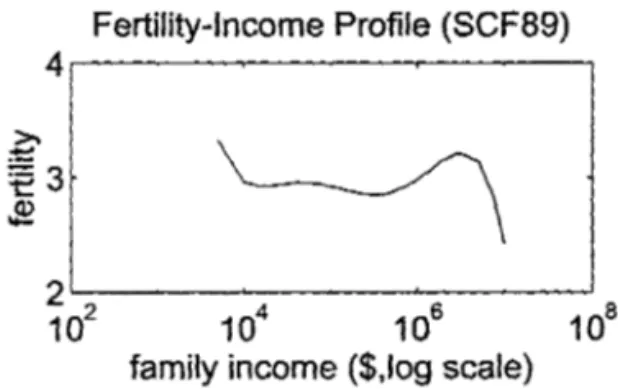
In addition to the evidence for Brazil provided in this paper, there is some evidence of a U-shaped fertility-income profile for other countries. Mulligan (1997) presents evidence for the

United States, using data from the 1990 U.S. Census and the 1989 Survey of Consumer

Finances.

Figure 8 displays the fertility-income cross-section relationship estimated in Mulligan

(1997) from the 1989 Survey of Consumer Finances. Mulligan uses number of children of

household heads between the ages of forty-one and eighty-four as his fertility measure. Both

plots displayed in Figure 8 were computed by fitting a fifth-order polynomial in log annual family income to the number of children. The top figure excludes childless families, as is

preferable in a study of persistence of inequality, and corresponds to the Brazilian

fertility-income relationship presented in Figure 7. The bottom figure includes childless families.

Fertility declines with income for family incomes up to US$ 300,000, and rises with

income for incomes between US$ 300,000 and US$ 3,000,000. Fertility declines with income

after US$ 3,000,000, but this is based on only thirty-three observations.

In addition to Mulligan (1997), Willis (1973) also provides evidence for the U.S., using

data from the 1960 U.s. Census. Ben-Porath (1973) presents evidence for Israel, using an

empirical model similar to Willis (1973).

The evidence on a concave relationship between adult child's income and father's income,

however, is mixed. In addition to the evidence provided in this paper, Mulligan (1993) also

found evidence of an inverse U-shaped relationship, but the regression coefficient on the

quadratic term is not significant. Both Behrman and Taubman (1990) and Solon (1992) found

evidence in the opposite direction, indicating a U-shaped relationship between adult child's and

parental income, but the regression coefficients also tend to be insignificant.

The mixed evidence on the shape of the cross-section investment-income profile may be

attributed to at least two reasons. First, with the exception of this paper, alI studies cited above

use small samples, which are not particularly suitable for a study of income -nonlinearities.

Second, from a theoretical standpoint the implication that the investment-income profile has a

concave pattem is less robust than the analogous implication for the fertility profile, because

investment is affected by other variables in addition to fertility.

The empirical evidence thus strongly supports the implications of the model regarding the

shape of the cross-section relationship between fertility and parental income, but is not

conclusive with respect the shape ofthe investment-income cross-section profile.

4.2. Evidence on the dynamic relationship between fertility and persistence of

inequality .

Another implication of the model is related to the dynamic behavior of the

fertility-wealth relationship, and its effect on the degree of intergenerational persistence of inequality.

fertility tends to become smaller as the country develops, reflecting a weaker cross-section

association between wealth and labor income over time. Moreover, the quantity-quality tradeoff

will tend to reduce the degree of persistence in inequality as the country develops.

In order to verify this implication of the model, I compare the degrees of persistence in

full-time wages and the coefficients obtained from a regression of fertility on wages for the 1976 PNAD and the Panel Study of Income Dynamics (PSID), where the U.S. regressions are taken

from Mulligan (1993).19 Mulligan uses information on father's wage rate and fertility taken from the period 1967-72, which makes the U.S. and Brazilian samples approximately contemporary.

Table 9 presents simple OLS regressions of fertility and adult child's wage on father's

wage, both for Brazil and the V.S. Both the fertility and persistence coefficients obtained from

the PNAD 76 are roughly the double (in absolute value) of their PSID counterparts. The results for the 1996 PNAD are not shown in Table 9, but they confirm the differences between Brazil and the U.S. For the 1996 sample, the coefficient on father's wage in the fertility regression is -2.10, whereas the wage coefficient in the mobility regression is 0.67.

Table 10 uses a procedure similar to the one used in Mulligan (1993) to estimate the quantitative importance of fertility decisions for the persistence of inequality across generations.

These regressions include as an explanatory variable the fitted value obtained from the

regression of mother's schooling on father's fertility, father's wage, age variables, a gender

durnmy and agriculture's share of personal income in the county where the son grew Up.20 The

idea is that the fitted value of mother's schooling controls for variations in the price of fertility

among families. The change in the coefficient on father's wage when the cost of children is

controlled for may then be interpreted as the contribution of fertility behavior for the persistence

of inequality.

19 Becker and Tomes (1986) present evidence from a dozen samples for the period 1960 through 1982 drawn from

five countries (V.S., England, Sweden, Switzerland, and Norway). They generally found low intergenerational persistence of inequality, averaging about 0.25. These low estimates may be downward biased, due to sample homogeneity and measurement error in parental income, but revised estimates for the V.S. eamings estimates are in

~eneral around 0.4, which is considerably smaller than the estimates for Brazil presented in the texto

o Because of data limitations, I use mother's labor income instead of parental fertility as an instrumento Also, for the same reason, I use a dummy variable indicating whether the father lives in a urban area, rather than agriculture share ofpersonal income in the county where the son grew up.

If we compare Tables 9 and 10, we can observe that the coefficient on father's wage in

1976 declines fifty-percent (from 0.76 to 0.38) when we control for the cost of children. The

corresponding decline in 1996 is of thirty-four percent (from 0.67 to 0.44). This is consistent

with the prediction that fertility becomes relatively less important as a source of inequality as the

country develops.

Table 10 also shows that the coefficient on father's wage for the U.S. declines forty-four

percent (fiom 0.36 to 0.20) when one controls for the cost of children. The relative importance of

fertility for persistence of inequality in the V.S. (around 1967-71) is thus slightly smaller then the

contemporaneous figure for Brazil. Since it is likely that other sources of inequality persistence

differ between Brazil and the V.S., it is probably more accurate to compare the absolute values

of the effect of fertility on inequality, rather than the percentage change. In this case, the impact

of fertility on persistence is much higher for Brazil (0.38) than the V.S. (0.16), which is

consistent with the model.

5. Conclusion

This paper analyzed the interaction between wealth composition, endogenous fertility and

the dynamics of wealth and income inequality, combining numerical simulations and empirical

evidence. The major fmdings of the paper may be summarized as follows.

The first set of findings relates cross-section relationships between parental wealth, on

the one hand, and wealth composition, fertility and investments per child, on the other. The

cross-section relationship between fertility and wealth tends to display a V-shaped pattem,

reflecting differences in the correlation between wealth and labor income among constrained and

unconstrained families. The interaction between quantity and quality of children implies a

concave cross-section relationship between investments per child and parental wealth.

The second set of fmdings is related to the dynamic behavior of the wealth and income

productivity of human capital investments are high relative to preferences for numbers of

children, alI families eventually overcome their borrowing constraints and there is long-run

equality among families. The negative effect of wealth on fertility declines as physical capital

becomes relatively more important as a source of wealth variations among families. The

quantity-quality tradeoff implies that the degree of persistence in income inequality tends to

decrease as the economy develops and families become unconstrained.

I provided empírical evidence on these two sets of implications using data from the

PNADs 76 and 96 and evidence taken from other studies. First, the evidence shows that the

fertility-income cross-section relationship tends to display a U-shaped pattem, as implied by the

modelo The cross-section relationship between adult child's income and parental income displays

a concave pattem, reflecting the interaction between quantity and quality of children.

Second, I provided evidence on the dynamic behavior of persistence of inequality by

comparing fertility behavior and persistence of income inequality between Brazil and the United

States. I found that the negative effect of income on fertility is larger in Brazil, which tends to

raise persistence of inequality in Brazil relative to the U.S. I also provided evidence that the

quantitative importance of fertility as a source of persistence of inequality declined in Brazil

between 1976 and 1996, which is consistent with the model.

The model constructed in this paper abstracts from several issues, in order to focus on the

mechanism relating wealth composition, fertility and investments per child. In particular, the

analysis does not consider the relationship between differences in fertility among skilled and

unskilled workers and the dynamic evolution of the wage premium, as in Kremer and Chen

(2000) and Doepke (2002). One interesting extension of the model would be to consider the

general equilibrium interaction between wealth composition, fertility and factor prices.

Another possible extension of the model would be to assume that investments per child

also require parental time, in addition to expenditures in goods. In this case, wealth composition

would affect investments both direct1y and through changes in fertility.

Also, Veloso (2002) provides evidence that differences in the allocation of time to

investments in children. This suggests that, in addition to the composition of income between

labor and nonlabor sources, the composition of household income between mother's and father's

References

Alvarez, Fernando (1999). "Social Mobility: The Barro-Becker Children Meet the

Laitner-Loury Dynasties." Review ofEconomic Dynamics 2: 65-103.

Becker, Gary S., and Robert Barro (1988). "A Refonnulation of the Economic Theory of

Fertility." Quarterly Journal of Economics 103: 1-25.

Becker, Gary S., and Nigel Tomes (1976). "Child Endowments and the Quantity and

Quality ofChildren." Journal ofPo/itical Economy84 (4), pt.2: SI43-S162.

Becker, Gary S., and Nigel Tomes (1986). "Human Capital and the Rise and Fall of

Families." Journal ofLabor Economics 4(3)(2):SI-S39.

Becker, Gary S., Kevin M. Murphy, and Robert F. Tamura (1990). "Economic Growth,

Human Capital, and Population Growth." Journal of Po/itical Economy 98:S12-S37.

Behnnan, Jere R. and Paul Taubman (1990). "The Intergenerational Correlation between

Children's Adult Earnings and their Parents' Income: Results from the Michigan Panel Survey of

Income Dynamics." Review oflncome and Wealth 36 (2):115-27.

Benhabib, Jess, and Kazuo Nishimura (1993). "Endogenous Fertility and Growth" in

General Equi/ibrium, Growth, and Trade lI, The Legacy of Lionel McKenzie. Edited by R.

Becker, M. Boldrin, R. Jones, and W. Thomson. Academic Press Inc.

Ben-Porath, Yoram (1973). "Economic Analysis of Fertility in Israel: Point and

Counterpoint." Journal ofPo/itical Economy 81 (2):S202-S233.

Dahan, Momo and Daniel Tsiddon (1998). "Demographic Transition, Income

Distribution, and Economic Growth." Journal of Economic Growth, 3:29-52.

Doepke, Matthias (2002). "Inequality and Growth: Why Differential Fertility Matters".

Working Paper, Department ofEconomics, VCLA.

Espenshade, Thomas J. (1977). "The Value and Cost of Children." Population Bul/etin

32 (1). Washington, DC, Population Reference Bureau.

Espenshade, Thomas J. (1984). Investing in Children: New Estimates of Parental

Galor, Oded and Omer Moav (2002). "From Physical to Human Capital Accumulation: Inequality and the Process ofDevelopment." Working Paper, Department ofEconomics, Brown University.

Greenwood, Jeremy, Nezih Guner and John A. Knowles (2002). "More on Marriage, Fertility and the Distribution of Income." International Economíc Revíew, forthcoming.

Hall, Robert E. and Charles I. Jones (1999). "Why do Some Countries Produce So Much More Output than Others?" Quarterly Journal of Economics 114 (F ebruary): 83-116.

Knowles, John (1999). "Social Policy, Equilibrium Poverty and Investment in Children." W orking Paper, Department of Economics, University of Pennsylvania.

Kremer, M. and Daniel Chen (2000). "Income Distribution Dynamics with Endogenous Fertility." NBER Working Paper 7530.

Laitner, John (1992). "Random Earnings Differences, Lifetime Liquidity Constraints, and Altruistic Intergenerational Transfers." Journal of Economíc Theory 58: 135-170.

Lam, David. (1986). "The Dynamics of Population Growth, Differential Fertility, and Inequality." American Economic Review. 76 (5): 1103-1116.

Leibowitz, Arleen (1974). "Education and Home Production." Amerícan Economic Review 64 (2):243-50

Loury, Glenn C. (1981). "Intergenerational Transfers and the Distribution of Earnings." Econometríca 49 (4):843-67.

Lucas, Robert E., Jr. (2002). Lectures on Economic Growth. Harvard University Press. Meltzer, David O. (1992). "Mortality Decline, the Demographic Transition, and Economic Growth." PhD. Dissertation, Department ofEconomics, University ofChicago.

Mulligan, Casey B. (1993). "Intergenerational Altruism, Fertility, and the Persistence of Economic Status." Ph.D. Dissertation, Department ofEconomics, University ofChicago.

Mulligan, Casey B. (1997). Parental Prioríties and Economíc Inequalíty. The University of Chicago Press.

Navarro-Zenneno, J. L (1993). "A Model of Bequests and Intergenerational Mobility."

PhD. Dissertation, Department ofEconomics, University ofChicago.

Palivos, Theodore (1995). "Endogenous Fertility, Multiple Growth Paths, and Economic

Convergence." Joumal ofEconomic Dynamics and Controll9: 1489-1510.

Solon, Gary (1992). "Intergenerational Income Mobility in the United States." American

Economic Review 82 (3): 393-408.

Tamura, Robert F. (1988). "Fertility, Human Capital and the "Wealth ofNations." PhD.

Dissertation, Department of Economics, University of Chicago.

Tamura, Robert F. (1994), "Fertility, Human Capital and the Wealth of Families."

Economic Theory 4: 593-603.

Veloso, Fernando (2002), "Income Composition, Endogenous Fertility and Schooling

Investments in Children." Working Paper, Department ofEconomics, Ibmec.

Willis, Robert J. (1973). "A New Approach to the Economic Theory of Fertility

Fertility Policy Function

physical capital

o

O

5

human capital

10

Figure 1-Fertility Policy Functions (baseline parameters)

Fertility Policy Function (k=2)

5~---~---.

5

human capital

10

Fertility Policy Function (h=2)

3,---~---.

>

-~2.5

2

5 10

~

cc .c

Labor-Share-Wealth Cross-Section Profile

1r---~----~~----~

~ 0.9

o .o

~

0.8'-0---~1----~2---' 3

10 10 10 10

parental wealth (Iog scale)

Fertility-Wealth Cross-Section Profile

4r---~---~---~

2L---~--~==~--~

100 101 102 103

parental wealth (Iog scale)

Figure 2-Cross-Section Profiles at t=O (baseline parameters)

-

Q) "ffi

C) Persistence of Wealth Inequality

~104r---~---~---~

o

:::::.. .c

~

Q) 102

~

"O

~10°'---~---~---'

::! _:::I 100 101 102 103

Fertility Policy Function

5 10

physical capital

o

O

human capital

Figure 3-Fertility Policy Functions (lambda=O.4)

Fertility Policy Function (k=2)

2~---~---.

~1.5f\

~ 1l~~

__________________

~

5

human capital

10

cn

-

c Q) E

(j)

~ 10

c

~ 5

.õ.

Physical Capital Policy Function

~18

~

5

₅ 10

P~ical

capital a.

O O

_{human capital}

Fertility Policy Function (h=2)

1.2

r----~---~---1

J

5

physical capital

~ ta

L:

Labor-Share-Wealth Cross-Section Profile

1r---~---~----~

~ 0.9

o

.o .!!1

0.8 o 1 2 3

10

10

10

10

parental wealth (Iog scale)

Figure 4-Cross-Section Profiles at t=O (lambda=O.4)

ã) (ti

u Persistence of Wealth Inequality

~104r---~---~----~

g

L:

~

_Q)

10

2

!;

"O

~ 100~---~---~----~

=:: _::J

10

0

10

1

10

2

10

3

-g

parental wealth (Iog scale)

Fertility-Wealth Cross-Section Profile

2r---~---~---~

O~---~---~----~

10

0

10

1

10

2

10

3

Fertility Policy Function

Fertility Policy Function (k=2) Fertility Policy Function (h=2)

5 3.5

~4

I~

>. ₃

~

:e

:e

~3 ~2.5

2 "- 2

O 5 10 O 5 10

Labor-Share-Wealth Cross-Section Profile

1.---~---~----~

~ ---~

co

.r:.

~ 0.9

o .c

~

0.8 o 1 2 3

10 10 10 10

parental wealth (Iog scale)

Figure 6-Cross-Section Profiles at t=O (epsilon=0.5)

-

Cl)

~

Persistence of Wealth Inequality

~104.---~---~----~

o ::::..

.r:.

~

10

2

-~ o-~

"fi

10 o 1 2 3

=s

10 10 10 10

-g

parental wealth (Iog scale)

Fertility-Wealth Cross-Section Profile

5r---~---~---~

O~---~---~----~

100 101 102 103

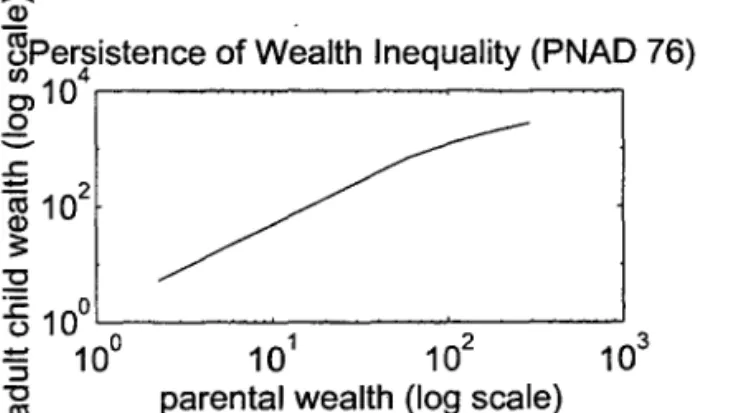
Fertility-Wealth Cross-Section Profile (PNAD 76)

10.---~---~---~

O~---~---~----~

10°

10

1

10

2

10

3

parental wealth (log scale)

Figure 7 -Cross-Section Profiles (PNAD 76)

-

(!)

~Persistence of Wealth Inequality (PNAD 76)

~104r---~---~----~

g

.!::

-;; 10

_(!) 2

~

"O

~100~---~---~----~

:!: _::::l

10°

10

1

10

2

10

3

Fertility-Income Profile without Childless (SCF89)

6~----~---~---~

~

2~----~---~---~

1~

1if

1~

1~

family income ($,Iog scale)

Figure 8-Fertility-lncome Cross-Section Profiles (SCF 89)

Fertility-Income Profile (SCF89)

4~----~---~---~

2~----~---~---~

1~

1if

1~

1~

Table 1: Baseline parameters

f3

= 0.25

r=3

e=O.2

A=5

 =0.14

a= 0.67

r

=0.33

Table 2: Fertility regression coefficients

(baseIine parameters)

wealth labor income

00 =-2.8 OOL =-2.6

O] =-2.2 O]L =-2.2

O2

=

-1.6 0/ =-1.6

0₃

=

-0.8 0/ =-0.8

04

=

O 0/=0

O~ =.

Table 3: Persistence of inequality

(baseline parameters)

persistence of weaIth persistence of labor income

Po = 0.82 _Po L =0.79

p] =0.67 p]L = 0.67

P2 =0.51 p/ =0.51

P3 =0.32 _P3 L =0.32

P4 = 0.l3 P4L =0.l3

Ps =0 _Ps L =0

Table 4: Fertility regression coefficients

(À =0.4)

wealth labor income

°

0 = -1.25 OOL =-1.22

OI = 0.01 0IL =0.01

l0'

=022 03 =0.89

Table 5: Persistence of inequality

(,1,=0.4)

persistence of wealth persistence of labor income

Po = 0.52 _Po L =0.45

PI =0.35 PIL =0.28

P2 = 0.19 p/ =0

P3 =0.16

L P3 =

P4 =0 P4 L =.

Table 6: Fertility regression coefficients

(e =0.5)

wealth labor income

(Jo = -2.95 (JOL =-2.80

(JI = -2.92 (JIL =-2.92

(J2 =-1.88 (J/ =-1.88

(J. = -0.92 (J3L =-0.92

(J4 = O (JL=O 4

Table 7: Persistence of inequality

(e=0.5 )

persistence of wealth persistence of labor income

Po = 0.93 Po L =0.91

PI =0.92 PIL =0.92

P2 = 0.95 p/ =0.95

P3 =0.98 _P3 L =0.98

P4 =1 P L-I 4

Table 8: OLS Regression of fertility, adult child's schooling and adult child's income on family income (full-time)- PNAD

96

independent

fertility adult child's adult child's

variables schooling income

parental income -3.18 * 10.17 * 2.14 *

(0.76) (0.58) (0.09)

parental income 0.17 * -0.86 * -0.13 *

squared (0.05) (0.05) (0.007)

adjusted R

0.17 0.48 0.57

squared

N 18227 17658 17658

Notes: (a) Ali income variable~ are measured in logs. Standard errors in parentheses. The regressions use sample weights provided by IBGE. N refers to the unweighted number of observations.

(b) The full-time concept of full income is defined as average family income for men who are household heads and work 40 hours per week on average. Different income averages are calculated for each possible combination af education category, state of residence and whether the individuallives in a urban or rural area.

(c) A constant, the mother's age, its age squared, the father's age, its age squared, the oldest child age, its age squared, the oldest child's sex, a dummy variable for urban areas and a dummy variable for the state in which the family resides are included in each regression.

Table 8: OLS Regression of fertility, adult child's schooling and adult child's income on family income (full-time)- PNAD

96

independent

fertility adult child's adult child's

variables schooling income

parental income -3.18 * 10.17 * 2.14 *

(0.76) (0.58) (0.09)

parental income 0.17 * -0.86 * -0.13 *

squared (0.05) (0.05) (0.007)

adjusted R

0.17 0.48 0.57

squared

N 18227 17658 17658

Notes: (a) Ali income variable~ are measured in logs. Standard errors in parentheses. The regressions use sample weights provided by IBGE. N refers to the unweighted number of observations.

(b) The full-time concept of full income is defined as average family income for men who are household heads and work 40 hours per week on average. Different income averages are calculated for each possible combination af education category, state of residence and whether the individuallives in a urban or rural area.

(c) A constant, the mother's age, its age squared, the father's age, its age squared, the oldest child age, its age squared, the oldest child's sex, a dummy variable for urban areas and a dummy variable for the state in which the family resides are included in each regression.

Table 9: OLS Regression of fertility and adult child's wage on father's wage (ful/-time)- PNAD 76 and Mulligan (1993)

independent fertifity adult child's wage fertility adult child's wage variables (PNAD 76) (PNAD 76) (Mulligan (1993» (Mulligan (1993)

father's wage -2.18 * 0.76 * -1.17 * 0.36 *

(0.04) (0.006) (0.16) (0.04)

adjusted R

0.18 0.46 0.1 0.21

squared

N 13384 20408 648 648

Notes: (a) Ali wage variables are measured in logs. Standard errors in parentheses. The PNAD regressions use sample weights provided by IBGE. N refers to the unweighted number of observations.

(b) The full-time wage measure for the PNAD is defined as average hourly wage for men who are household heads and work 40 hours per week on average. Different wage averages are

calculated for each possible combination of education category, state of residence and whether the individual lives in a urban or rural area.

(c) A constant, the father's age, its age squared, the child's age, its age squared and the child's sex are included in each regression, and a dummy variable indicating whether the father lives in a urban area (Brazif).

Table 10: 2SLS Regression of fertility and adult child's wage on father's wage (full-time)- PNAD 76, PNAD 96 and Mulligan

(1993)

independent adult child's wage adult child's wage adult child's wage

variables (PNAD 76) (PNAD 96) (Mulligan (1993)

father's wage 0.38 * 0.44* 0.20 **

(0.01) (0.01) (0.11 )

mother's schooling 0.07 * 0.03* 0.06

(0.003) (0.001) (0.05)

adjusted R

0.46 0.45 0.21

squared

N 16380 34889 648

Notes: (a) Ali wage variables are measured in logs. Standard errors in parentheses. The PNAD regressions use sample weights provided by IBGE. N refers to the unweighted number of observations.

(b) The full-time wage measure for the PNAD is defined as average hourly wage for men who are household heads and work 40 hours per week on average. Different wage averages are calculated for each possible combination of education category, state of residence and whether the individual lives in a urban or rural area.

(c) For the Mulligan (1993) PSID data mother's schooling is the fitted value trom a

regression of mother's schooling on the age variables, father's wage, fertility, a gender dummy and agriculture's share of personal income in the county where the son grew up. For the PNAD, mother's schooling is the fitted value from a regression of mother's schooling on the age variables, father's wage, mother's full-time labor income, a gender dummy , and a dummy variable indicating whether the father lives in a urban area.

(d) A constant, the father's age, its age squared, the child's age, its age squared and t

(e) * significant at the one-percen! levei

• . • li L I . T" ~ A""

J

~Millll\)l IlilIEINlRIIOIIJJE ~'MON~N "

J~11CA1 &uÍÍl~ _,,~\ ~ ..

!

!