Results from a new linear O<sub>3</sub> scheme with embedded heterogeneous chemistry compared with the parent full-chemistry 3-D CTM

(1)

ACPD

10, 12993–13027, 2010

Stratospheric ozone scheme from 3-D

CTM

B. M. Monge-Sanz et al.

Title Page

Abstract Introduction

Conclusions References

Tables Figures

◭ ◮

Back Close

Full Screen / Esc

Printer-friendly Version Interactive Discussion

Discussion

P

a

per

|

Dis

cussion

P

a

per

|

Discussion

P

a

per

|

Discussio

n

P

a

per

|

Atmos. Chem. Phys. Discuss., 10, 12993–13027, 2010 www.atmos-chem-phys-discuss.net/10/12993/2010/ doi:10.5194/acpd-10-12993-2010

Atmospheric Chemistry and Physics Discussions

This discussion paper is/has been under review for the journal Atmospheric Chemistry and Physics (ACP). Please refer to the corresponding final paper in ACP if available.

Results from a new linear O

₃

scheme with

embedded heterogeneous chemistry

compared with the parent full-chemistry

3-D CTM

B. M. Monge-Sanz1, M. P. Chipperfield1, D. Cariolle2,3, and W. Feng1

1

Institute for Climate and Atmospheric Science, School of Earth and Environment, University of Leeds, Leeds, UK

2

Centre Europ ´een de Recherche et Formation Avanc ´ee en Calcul Scientifique, Toulouse, France

3

M ´et ´eo-France, Toulouse, France

Received: 23 April 2010 – Accepted: 5 May 2010 – Published: 20 May 2010 Correspondence to: B. M. Monge-Sanz (beatriz@env.leeds.ac.uk)

(2)

ACPD

10, 12993–13027, 2010

CTM

Title Page

Tables Figures

◭ ◮

Back Close

Full Screen / Esc

Discussion

P

a

per

|

Dis

cussion

P

a

per

|

Discussion

P

a

per

|

Discussio

n

P

a

per

Abstract

A detailed full-chemistry 3-D chemistry and transport model (CTM) is used to evalu-ate the current stratospheric O₃parameterisation in the European Centre for Medium-Range Weather Forecasts (ECMWF) model and to obtain an alternative version of the ozone scheme implicitly including heterogeneous chemistry. The approach avoids the

5

inaccurate treatment currently given to heterogeneous ozone chemistry in the ECMWF model, as well as the uncertainties of a cold-tracer. The new O₃scheme (COPCAT) is evaluated within the same CTM used to calculate it. It is the first time such a compari-son has been possible, providing direct information on the validity of the linear param-eterisation approach for stratospheric ozone. Simulated total column and O₃ profiles

10

are compared against Total Ozone Mapping Spectrometer (TOMS) and Halogen Occul-tation Experiment (HALOE) observations. COPCAT successfully simulates polar loss and reproduces a realistic Antarctic O₃hole. The new scheme is comparable to the full-chemistry in many regions for multiannual runs. The parameterisation produces less ozone over the tropics around 10 hPa, compared to full-chemistry and observations,

15

however, this problem can be ameliorated by choosing a different ozone climatology for the scheme. The new scheme is compared to the current ECMWF scheme in the same CTM runs. The Antarctic O₃hole with the current ECMWF scheme is weaker and disappears earlier than with the new COPCAT scheme. Differences between the cur-rent ECMWF scheme and COPCAT are di_fficult to explain due to the di_fferent approach

20

used for heterogeneous chemistry and di_fferences in the photochemical models used to calculate the scheme coefficients. Results with the new COPCAT scheme presented here show that heterogeneous and homogeneous ozone chemistry can be included in a consistent way in a linear ozone parameterisation, without any additional tunable parameters, providing a parameterisation scheme in much better agreement with the

25

(3)

ACPD

10, 12993–13027, 2010

CTM

Title Page

Tables Figures

◭ ◮

Back Close

Full Screen / Esc

Discussion

P

a

per

|

Dis

cussion

P

a

per

|

Discussion

P

a

per

|

Discussio

n

P

a

per

|

1 Introduction

Numerical weather prediction (NWP) models cannot yet a_fford to include detailed chemistry schemes, although a realistic representation of radiatively active species is essential for the correct assimilation of satellite radiances into these models. NWP systems must therefore make use of simplified parameterisations of the species most

5

relevant to them, i.e. radiatively active gases such as O₃, H₂O, CH₄ and CFCs. In the last two decades, the Cariolle and D équ é (CD) scheme (Cariolle and D équ é, 1986; Cariolle and Teyss èdre, 2007) has been the most widely used parameterisation for stratospheric ozone. McCormack et al. (2006) gives a summary of the evolution of the ozone schemes implemented by global models before the numerical CD approach

10

appeared as a more suitable option. The CD scheme represents the time tendency of ozone as a function of production (P_{) and loss (}L_{), where the net production (}P₋L_{) is} considered a linear function of ozone mixing ratio (f_{), temperature (}T_{) and partial} col-umn of ozone above the considered point (c_O

3). The coefficients for the linearisation are obtained from a photochemical model and provided as look-up tables which are

15

function of latitude, level and month of the year. The photochemical models used until now to derive the coe_fficients have included only gas-phase chemistry (Cariolle and D équ é, 1986; Cariolle and Teyss èdre, 2007; McCormack et al., 2006) or very limited heterogeneous processes (McLinden et al., 2000), which has made it necessary to include an additional term in the parameterisation to take into account heterogeneous

20

chemistry.

The European Centre for Medium-Range Weather Forecasts (ECMWF) model uses a linear parameterisation for O₃ based on the CD approach. The O₃ coe_fficients for the CD scheme used by the ECMWF model (Dethof and H ´olm, 2004) come from the 2-D photochemical model MOBIDIC (Cariolle and Teyss `edre, 2007). The complete

25

ECMWF scheme is based on the expression ∂f

∂t=c0+c1(f−f¯)+c2(T−T¯)+c3(cO3−c¯O3)+c4(ClEQ)

(4)

ACPD

10, 12993–13027, 2010

CTM

Title Page

Tables Figures

◭ ◮

Back Close

Full Screen / Esc

Discussion

P

a

per

|

Dis

cussion

P

a

per

|

Discussion

P

a

per

|

Discussio

n

P

a

per

where ¯f_{, ¯}T _{and ¯}c_O

3 are climatological reference values for local O3, temperature and partial column of O₃. The coefficientsc_i ₍i₌_{0, 1, 2, 3, 4) are obtained with the} pho-tochemical model. The fifth term on the right hand side of Eq. (1) corresponds to the additional heterogeneous term used in the current ECMWF parameterisation. Cl_EQ is the equivalent chlorine content of the stratosphere, and is the only parameter that

5

varies from year to year. This fifth term is only active when temperature falls below 195 K in daytime for latitudes poleward of 45◦. This ECMWF ozone scheme version (currently operational) is also denoted here v2.9 after the version of coefficients pro-vided by M ´et ´eo France. Other versions following the same conceptual CD approach are LINOZ (McLinden et al., 2000) and CHEM2D (McCormack et al., 2004, 2006). Geer

10

et al. (2007) gives a comparison of several versions of ECMWF, LINOZ and CHEM2D coe_fficients in terms of their performance in a data assimilation system. However, none of these schemes includes a complete heterogeneous description, and all of them need an extra term for the simulation of O₃ polar loss. In Geer et al. (2007) heterogeneous processes were parameterised by means of a cold tracer (Eskes et al., 2003) for all the

15

evaluated O₃schemes.

The CD scheme first appeared in the 1980s, when knowledge of the importance of heterogeneous O₃ chemistry was very limited. Therefore, in its original version the CD parameterisation lacked a heterogeneous term. More recent versions (Cariolle and Teyss `edre, 2007) were computed in a similar way to their predecessor: omitting

hetero-20

geneous chemistry but including an additional term calculated with di_fferent methods and approximations and, thus, not consistent with the gas-phase chemistry described by the scheme. This separation between gas-phase and heterogeneous reactions, as discussed in Sect. 1 reduces the accuracy of the ECMWF approach. The alternative of using a cold tracer, which has been presented as an improvement to the current

25

(5)

ACPD

10, 12993–13027, 2010

CTM

Title Page

Tables Figures

◭ ◮

Back Close

Full Screen / Esc

Discussion

P

a

per

|

Dis

cussion

P

a

per

|

Discussion

P

a

per

|

Discussio

n

P

a

per

|

Here a new approach is proposed and evaluated. Based on the CD linear approach, a new set of coe_fficients is obtained from a 3-D CTM including complete heteroge-neous processes. The alternative ozone scheme COPCAT (Coefficients for Ozone Pa-rameterisation from a Chemistry And Transport model) does not need any additional heterogeneous term as it implicitly includes heterogeneous chemistry in the first 4

coef-5

ficients (Monge-Sanz, 2008). This is a more natural way to include both gas-phase and heterogeneous processes, not only at polar latitudes but also over mid/low latitudes, where the CD scheme unrealistically neglects any heterogeneous e_ffect. In addition, from existing literature it is difficult (if not impossible) to discern whether the limitations of the ozone schemes come from the parameterisation approach or from the

photo-10

chemical model used to obtain the coe_fficients, or even from the 3-D model where the scheme is implemented. Obtaining a new scheme based on TOMCAT/SLIMCAT (Chip-perfield, 2006), a widely used and evaluated 3-D CTM, helps to clarify which problems are due to the parameterisation approach as distinct from the limitations of the parent photochemical model. This study presents the first comparison between a linear ozone

15

parameterisation and the equivalent full chemistry 3-D model used to calculate it. The main di_fference between the COPCAT scheme proposed here and the current ECMWF scheme is in the treatment of the heterogeneous chemistry. Using a localised heterogeneous term (i.e. the 5th term in Eq. 1) produces too weak polar ozone loss in the ECMWF global model, unless O₃ observations are assimilated (Dethof and H ´olm,

20

2004). Conceptually, this kind of term is too restrictive with respect to the current un-derstanding of heterogeneous processes. First, the temperature threshold for the for-mation of polar stratospheric clouds (PSCs) actually depends on altitude and trace gas concentrations. The adopted sharp threshold temperature of 195 K in Eq. (1) is repre-sentative of an altitude of∼20 km and 5 ppbv1HNO3(e.g. Hanson and Mauersberger, 25

1988; Carslaw et al., 1994). For a more realistic scheme, the temperature threshold in the heterogeneous term should include altitude dependency, and whenever possible be linked to the concentrations of H₂O, HNO₃ and H₂SO₄ aerosol. Second, another

1

(6)

ACPD

10, 12993–13027, 2010

CTM

Title Page

Tables Figures

◭ ◮

Back Close

Full Screen / Esc

Discussion

P

a

per

|

Dis

cussion

P

a

per

|

Discussion

P

a

per

|

Discussio

n

P

a

per

fundamental shortcoming of the heterogeneous approach in Eq. (1) is that it assumes chlorine activation and O₃ destruction by sunlight to take place at the same time. In reality, the activation of air masses takes place during the polar night inside the polar vortex, when temperature is low enough. Later, with the return of spring sunlight to po-lar latitudes, the processed air is able to destroy ozone. However, the destruction can

5

also happen during winter if activated air masses can reach lower latitudes (e.g. by fila-mentation or vortex break-up) and be exposed to sunlight. This latter kind of process is completely missed by a localised temperature term like the one in the ECMWF scheme (Eq. 1). A more realistic approach would be the use of a cold-tracer (e.g. Chipperfield et al., 1994; Cariolle and Teyss `edre, 2007). With this kind of approach, the model

10

keeps memory of the quantity of air processed by PSCs and of the amount of time that air has been subsequently exposed to sunlight. The cold-tracer approach is there-fore able to propagate the O₃destruction to areas outside the region where PSCs are formed, i.e. outside the restricted (T <195 K) region. This is particularly relevant for the Arctic, due to the vortex being less stable than its Antarctic counterpart. A cold-tracer

15

can therefore be more realistic than the ECMWF heterogeneous term, but this kind of tracer requires an accurate tuning (of activation and deactivation parameters) in or-der to provide realistic O₃destruction and, as meteorological and chemical conditions change, the same cold-tracer parameters would not be equally valid for every year.

Finally, for the long-term evolution of polar ozone loss, the actual heterogeneous

20

chemistry loss is not proportional to the square of the chlorine content (Cl2_EQ). As shown by Searle et al. (1998), an exponent value of 1.5 is much more representative of the typical conditions encountered in a fully activated polar vortex. In addition, not only do chlorine cycles play a role in destroying polar ozone, the ClO₊BrO cycle can account for up to 50% of the polar depletion, and for this latter cycle the Cl dependency is

25

(7)

ACPD

10, 12993–13027, 2010

CTM

Title Page

Tables Figures

◭ ◮

Back Close

Full Screen / Esc

Discussion

P

a

per

|

Dis

cussion

P

a

per

|

Discussion

P

a

per

|

Discussio

n

P

a

per

|

used for earlier years the quadratic dependence on Cl will decrease making the ozone loss even smaller compared to observations.

A better option that represents a good compromise between a realistic heteroge-neous full-chemistry and a simple one-tracer scheme is the use of a scheme of the form described in Eq. (1) but, instead of using the additional 5thterm, using an

alterna-5

tive set of coefficients (c₀_,c₁_,c₂ _andc₃_{) that implicitly include heterogeneous ozone} chemistry. Not only is this expected to improve the representation of polar ozone, but has also the advantage of including mid-latitude heterogeneous processes that have been so far ignored by most O₃linear schemes. This approach has been explored in this study, where a set of coefficients with implicit heterogeneous chemistry has been

10

calculated and tested with SLIMCAT CTM runs. For this approach long-term changes in stratospheric chlorine (or odd nitrogen, water vapour etc.) can be taken into account in a consistent way by deriving coefficients from the CTM for different periods.

In this paper, Sect. 2 describes the calculation of the new COPCAT scheme. The observations used to validate model results are briefly described in Sect. 3. The

pa-15

rameterisation performance is shown in Sect. 4, where the new scheme is compared with SLIMCAT full-chemistry runs and the current ECMWF scheme within CTM runs. This section also includes further polar results showing the ability of COPCAT to adapt to different meteorological conditions. A final summary of results and future work and applications is given in Sect. 5.

20

2 COPCAT scheme

2.1 Coefficients calculation

To calculate the parameterisation coefficients, the TOMCAT box model was initialised with the zonally averaged output of a full-chemistry simulation of the SLIMCAT 3-D model (Chipperfield, 2006) run 323. Run 323 is a multiannual SLIMCAT run that uses

25

a 7.5◦

(8)

ERA-ACPD

10, 12993–13027, 2010

CTM

Title Page

Tables Figures

◭ ◮

Back Close

Full Screen / Esc

Discussion

P

a

per

|

Dis

cussion

P

a

per

|

Discussion

P

a

per

|

Discussio

n

P

a

per

40 winds (Uppala et al., 2005) from 1977–2001 and by ECMWF operational winds from 2002–2006. The period chosen to initialise the box model corresponds to January– December 2000. From the initial state seven 2-day runs of the box model were carried out; one control run and six perturbation runs from the initial conditions. The resolution adopted for the box model is 24 latitudes, and 24 levels (from the surface up to_∼60 km),

5

matching the resolution of the full-chemistry run used for the initialisation. The box model also uses the same chemistry module as the full SLIMCAT model. The short runs of the CTM in box model mode were used to compute the ozone tendencies in the COPCAT scheme (Monge-Sanz, 2008). In these runs the chemistry was computed every 20 min.

10

The coe_fficients corresponding to the climatological (reference) values in Eq. (1), i.e.f,T andc_O

3, are directly provided by the zonal output of the SLIMCAT initial state on the 15th of each month. For the four photochemical coe_fficients (c_i) linear tendencies for the net ozone production (P₋L_{) were calculated from the corresponding box model} runs. Tendencies are calculated for odd oxygen O_x and then scaled by the factor

15

[O₃]/[O_x] to obtain the O₃ coe_fficients. One control run (using the unperturbed zonal initial values) was used to obtain the reference net productionc₀₌₍P₋L₎₀_{. For the} three coe_fficients given by the partial derivatives, the initial values off,T andc_O

3 are perturbed, one at a time, to obtain the corresponding linear tendency in (P₋L). The values used for the perturbations are ±5% for local ozone and column above, and 20

±4 K for temperature, the same perturbation values as in McLinden et al. (2000). The

coe_fficients are based on the daily net production of O₃ averaged over the last day of the run (second day in this case). For the ozone perturbed runs (local ozone and column), O₃ on the second day of the run is initialised with the average field over the first day. The whole calculation procedure is applied to every month of the year. This

25

(9)

ACPD

10, 12993–13027, 2010

CTM

Title Page

Tables Figures

◭ ◮

Back Close

Full Screen / Esc

Discussion

P

a

per

|

Dis

cussion

P

a

per

|

Discussion

P

a

per

|

Discussio

n

P

a

per

|

a tracer following the COPCAT approach ∂f

∂t=c0+c1(f−f¯)+c2(T−T¯)+c3(cO3−c¯O3) (2) 2.2 Implicit heterogeneous chemistry

A 3-D model using COPCAT coe_fficients can successfully simulate polar and mid-latitude O₃depletion despite the fact that no additional heterogeneous term is included.

5

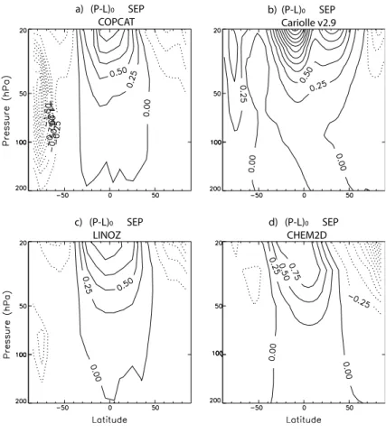
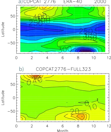
By plotting the September reference net production (P₋L₎₀_{, i.e.}c₀_{, in the lower} strato-sphere (LS) for the di_fferent schemes (Fig. 1), it can be seen that COPCAT shows a depletion region centred at 50 hPa over the south pole. This represents the ozone destruction caused by PSCs triggered by spring sunlight. None of the other schemes shows such a depletion region; only LINOZ shows a weak loss region at 100 hPa over

10

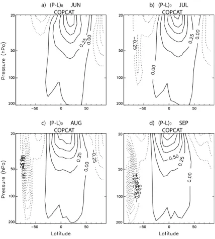
southern high latitudes, but it is not enough to produce spring ozone depletion over the Antarctic. Figure 2 shows the evolution of COPCATc₀_coe_ffi_{cient in June–September} in the LS. The Antarctic loss region starts to develop at the edge of the vortex in July; in September values of₋2.1 ppmv/month are reached around 40 hPa at high southern latitudes.

15

2.3 Linearity validation

Despite the nonlinear interactions involved in O₃ chemistry (both gas-phase and het-erogeneous), the validity of the linear approximation in previous schemes based on the CD approach has been shown in the literature. For the original version (Cariolle and D ´equ ´e, 1986) the di_fferences between the linear tendency inf and the real tendency

20

(in the 2-D model) were found to be less than 1% for variations of_±20% in the value of f_{. For LINOZ, McLinden et al. (2000) showed the deviations from the linear tendencies} in (P ₋L) with respect tof,c_O

3 and T, such deviations were low enough to consider the linear approximation valid for the usual range of variability observed in GCMs. Also, McCormack et al. (2006) showed the linearity in CHEM2D was valid for variations of

(10)

ACPD

10, 12993–13027, 2010

CTM

Title Page

Tables Figures

◭ ◮

Back Close

Full Screen / Esc

Discussion

P

a

per

|

Dis

cussion

P

a

per

|

Discussion

P

a

per

|

Discussio

n

P

a

per

±20 K in temperature and±50% in ozone column. Analysing the linear approximation

in the COPCAT scheme is also necessary, since the previous schemes did not include any polar heterogeneous chemistry implicitly, and only LINOZ included processes on binary sulfate aerosols.

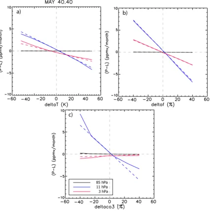
Figure 3 shows the COPCAT (P ₋L_{) values as a function of perturbation of local}

5

ozone f, temperature T and column above c_O

3 for three vertical levels, at 40

◦_{N in}

May. The range of variation, with respect to the reference state, chosen for the three variables are±40% in local ozone and column and±16 K in temperature. The vertical

levels represented correspond to 85 hPa, 11 hPa and 3 hPa. The exact tendency has been represented together with the linear squares fit to the points used to obtain the

10

COPCAT coefficients. The linearisation is a good approximation for the three variables in the shown ranges and only the dependence withc_O

3 shows some non-linearity for column variations larger than±20%.

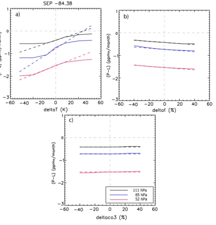
The level of agreement with the linear approximation shown in Fig. 3 is similar for other months and latitudes, except for polar LS regions in spring. Figure 4 evaluates the

15

linear approximation in the LS at 84◦S in September. The linearity of the scheme is still good for the O₃variables (local and column above), however, variations in temperature larger than 10 K take (P₋L) outside the linear COPCAT range. From Fig. 4a it can be seen that the control run in the coefficients calculation (∆T ₌_{0) is already under} PSC conditions (negative (P₋L_{)); further lowering T causes more ozone loss, while}

20

increasingT reduces the amount of loss. Note that the figure shows that the threshold for further PSC activation due to denitrification is not a sharp step but more of a smooth threshold. Chlorine activation on cold sulfate aerosol near the PSC formation threshold causes activation rates to vary in this way.

These results show that the linear approximation is also a good estimation for the O₃

25

scheme developed here. Despite including heterogeneous chemistry implicitly COP-CAT agrees with a linear approximation for local ozone variations of up to±40%,

col-umn ozonec_O

(11)

po-ACPD

10, 12993–13027, 2010

CTM

Title Page

Tables Figures

◭ ◮

Back Close

Full Screen / Esc

Discussion

P

a

per

|

Dis

cussion

P

a

per

|

Discussion

P

a

per

|

Discussio

n

P

a

per

|

lar loss. To ensure that the variations are within the ranges considered above, attention must also be paid to the choice of the reference states (or climatologies). The inclusion of higher order terms for the temperature dependency can be considered as a future improvement to further ensure the accuracy of the scheme in polar regions.

3 Ozone observations

5

We compare model results in this work against Total Ozone Mapping Spectrometer (TOMS) column observations (McPeters et al., 1998), and O₃ data from the Halogen Occultation Experiment (HALOE) (Br ¨uhl et al., 1996).

3.1 TOMS data

TOMS provided a near-continuous record of ozone measurements from 1978 to

De-10

cember 2005, with a high-density horizontal coverage of total ozone of about 200 000 observations per day (only daylight measurements). TOMS data have been widely used for the validation of models and other observational sets. Monthly data of TOMS Earth Probe (EP) (McPeters et al., 1998) have been obtained from http://toms.gsfc. nasa.gov/. Zonal monthly means are available from 85◦_N–85◦_{S with a 5}◦_resolution. 15

3.2 HALOE O3data

HALOE O₃ monthly data have been provided by W. Randel and F. Wu (from NCAR, USA) and correspond to the version 19 of HALOE public data release. These HALOE data are zonally averaged and are available for 41 latitudes (80◦_N–80◦_{S) and 49}

pres-sure levels (from 100–0.01 hPa). HALOE data have very high vertical resolution (2 km),

20

(12)

ACPD

10, 12993–13027, 2010

CTM

Title Page

Tables Figures

◭ ◮

Back Close

Full Screen / Esc

Discussion

P

a

per

|

Dis

cussion

P

a

per

|

Discussion

P

a

per

|

Discussio

n

P

a

per

4 Performance of the COPCAT scheme

The way COPCAT coefficients have been calculated enables for the first time the com-parison between the parameterisation and the full-chemistry CTM used to obtain it. In this way, the same numerics and dynamics are involved and di_fferences can only be due to the use of the COPCAT scheme instead of the full-chemistry. This kind of

5

evaluation was not possible for previous linear O₃ parameterisations, since they were computed by 2-D photochemical models and then implemented within 3-D GCMs or CTMs.

4.1 Comparison with full-chemistry simulations

The SLIMCAT full-chemistry run 323 is in good general agreement with TOMS

(Monge-10

Sanz, 2008) and the temporal and spatial evolution of O₃is well simulated. In particular, the minimum in the southern hemisphere spring is accurately represented by SLIM-CAT in multiannual runs (e.g. Chipperfield, 1999, 2003). Figure 5 shows the January– December 2000 total ozone (TO) column simulated by COPCAT and di_fferences with respect to the full-chemistry run 323. The two CTM runs use ERA-40 winds, same

15

resolution and advection schemes; the only difference between COPCAT and run 323 is in the chemistry. Results over the tropics and mid-latitudes are almost identical. The main di_fferences are over high latitudes, where COPCAT values are larger than the full-chemistry, indicating that the parameterisation scheme underestimates polar ozone loss compared to the full 3-D CTM. In the SH di_fferences remain low (<20 DU2) for all

20

months except in late winter and early spring (i.e. early in the ozone hole season), when COPCAT gives values up to 40 DU higher than the full-chemistry. The situa-tion over the Arctic is very similar, di_fferences are below 20 DU except in winter/spring. However, maximum di_fferences over the Arctic are larger than in the Antarctic, reaching up to 60 DU in March.

25

2

(13)

ACPD

10, 12993–13027, 2010

CTM

Title Page

Tables Figures

◭ ◮

Back Close

Full Screen / Esc

Discussion

P

a

per

|

Dis

cussion

P

a

per

|

Discussion

P

a

per

|

Discussio

n

P

a

per

|

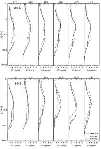
Total ozone column is a good diagnostic for the global variability achieved by the model both in time and space. However, the vertical distribution of O₃ must also be realistic in order to simulate correct radiative fluxes at all levels in the atmosphere. Figure 6 shows vertical profiles at 84◦N (February–July) and 84◦S (July–December), obtained with the COPCAT parameterisation and full-chemistry SLIMCAT runs driven

5

by ERA-40 2000 winds. The O₃destruction in spring between 30–100 hPa is success-fully simulated by COPCAT. However, the ozone hole duration is much shorter in the parameterisation than in the full-chemistry. The parameterisations, both COPCAT and the operational ECMWF scheme, tend to overestimate O₃in the mid/low stratosphere at high southern latitudes. The same occurs at 84◦N during winter and spring. In the

10

upper stratosphere, compared to full-chemistry, the parameterisations underestimate O₃ in spring. The agreement for the O₃ profiles over the tropics (Fig. 7) is very good except for the fact that the maximum value around 10 hPa is underestimated by the parameterisation. If the COPCAT ¯f reference state is replaced with that included in the CHEM2D scheme, which corresponds to the Fortuin and Kelder (1998) O₃

clima-15

tology, then O₃ values above 5 hPa increase (green line in Fig. 7). This shows that using a different O₃ climatology affects the maximum peak value over the tropics and adds ozone above 5 hPa, compared to the run using the default COPCAT ¯f (solid black line in Fig. 7). This proves the relevance of the climatology/reference state choice, us-ing the CHEM2D climatology improves results at low/mid latitudes and differences with

20

TOMS are reduced (Fig. 8c). However, the Antarctic ozone depletion is less realistic with this climatology; the minimum in September–October is around 60 DU higher with the CHEM2D climatology.

4.2 Comparison versus ECMWF v2.9

Both COPCAT and the ECMWF scheme are based on the same linear CD approach

25

(14)

ACPD

10, 12993–13027, 2010

CTM

Title Page

Tables Figures

◭ ◮

Back Close

Full Screen / Esc

Discussion

P

a

per

|

Dis

cussion

P

a

per

|

Discussion

P

a

per

|

Discussio

n

P

a

per

to model the heterogeneous chemistry effects over the poles. The COPCAT scheme is here compared in detail with the current ECMWF operational scheme in SLIMCAT 3-D runs.

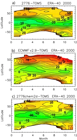
Figure 8 shows total O₃column differences between SLIMCAT runs using COPCAT and ECMWF ozone schemes and TOMS for year 2000. Over the tropics both schemes

5

underestimate column values, COPCAT simulating up to 30 DU less than observed and v2.9 up to 20 DU less. Over northern mid and high latitudes the differences are particularly large for the ECMWF scheme, which clearly overestimates column values compared to TOMS. In the Antarctic, both schemes overestimate TO column, except in Oct-Dec, when COPCAT underestimates ozone column values by 10–20 DU. Further

10

comparisons at polar latitudes are discussed in Sect. 4.3.

Like COPCAT, the ECMWF scheme underestimates the tropical maximum with re-spect to full chemistry (Fig. 7). Nevertheless, ECMWF ozone is∼1 ppmv larger than

COPCAT above 5 hPa. The annual mean zonal mean ECMWF O₃ distribution (fig-ure not shown) also confirms this; the ECMWF O₃ maximum centred at 10 hPa is

15

larger than in the COPCAT simulation for all latitudes, although lower than the full-chemistry run over tropics and mid-latitudes. At NH high latitudes (Fig. 6) the ECMWF scheme simulates too high O₃ in the mid/lower stratosphere compared to both the full-chemistry and COPCAT; up to 2 ppmv higher in June–July. The differences in the mid/lower stratosphere between ECMWF ozone and COPCAT or full-chemistry are

20

larger in the Antarctic region. From September to November the ECMWF scheme in the LS (∼100 hPa) is larger than the SLIMCAT full-chemistry or the COPCAT

param-eterisation (lower panel in Fig. 6). This helps to explain why the ozone hole is not as deep with the ECMWF scheme as it is with COPCAT or SLIMCAT full-chemistry (Fig. 8 and Sect. 4.3). Vertical features above 100 hPa also differ, with ECMWF O₃

25

being larger overall and showing too fast a recovery of the O₃hole, similar to COPCAT compared to the full-chemistry.

(15)

ACPD

10, 12993–13027, 2010

CTM

Title Page

Tables Figures

◭ ◮

Back Close

Full Screen / Esc

Discussion

P

a

per

|

Dis

cussion

P

a

per

|

Discussion

P

a

per

|

Discussio

n

P

a

per

|

the ECMWF and COPCAT schemes might be playing the fundamental role in explaining the di_fferences between both schemes. At high latitudes, the di_fferent heterogeneous chemistry treatment is the most probable cause of discrepancy between the schemes. However, at mid-latitudes both factors play important roles and it is difficult to attribute the main cause of the di_fferences.

5

4.3 Polar winter/spring O₃with COPCAT

This section compares the ability of the COPCAT scheme to simulate O₃ destruction at high latitudes with that of the full-chemistry CTM and the ECMWF scheme including the heterogeneous term in Eq. (1). It also shows the ability of COPCAT to adapt to different meteorological conditions (cold/warm polar winters).

10

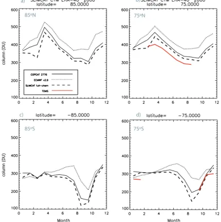
Figure 9a and b show TO column January–December 2000 at 85◦N and 75◦N, re-spectively for SLIMCAT simulations using the COPCAT scheme, the ECMWF scheme and the full-chemistry. The two parameterisations result in too large column values compared to the full-chemistry and TOMS. The ECMWF scheme results in the highest column values, 30 DU higher than COPCAT on average over high NH latitudes and

15

∼80 DU higher than TOMS at 75◦N. In the Antarctic COPCAT column values are very

close to full-chemistry (Fig. 9c and d). The ozone hole in September-October is better represented by COPCAT than by the ECMWF scheme which, except for the summer months, results in column values much larger than the other two runs (full-chemistry and COPCAT). Based on the few TOMS observations available at 75◦S both COPCAT

20

and SLIMCAT simulate a realistic ozone hole. These results are a further proof of the suitability of the implicit heterogeneous chemistry approach. The high column values obtained with the ECMWF scheme in the Antarctic region during winter (Fig. 9c and d) can in part be explained by transport of ozone from higher altitudes. In the Antarctic region the ECMWF scheme concentrations above 50 hPa are significantly higher than

25

(16)

ACPD

10, 12993–13027, 2010

CTM

Title Page

Tables Figures

◭ ◮

Back Close

Full Screen / Esc

Discussion

P

a

per

|

Dis

cussion

P

a

per

|

Discussion

P

a

per

|

Discussio

n

P

a

per

rate of decrease for the period of sharp ozone decline is similar for both schemes, the COPCAT scheme, as well as the full-chemistry run, already starts to show some de-cline in late winter due to the ongoing loss at the edge of the vortex; this loss process is missed by the heterogeneous treatment in the current ECMWF scheme. The implicit calculation approach in the new COPCAT scheme makes it less vulnerable to transport

5

problems and able to achieve realistic chemical loss at the edge of the polar vortex. The coefficients for this kind of linear parameterisations based on the CD approach are calculated under certain atmospheric conditions, both chemical and meteorologi-cal. In the case of COPCAT such conditions correspond to the year 2000. However, the amount of O₃ loss, especially in the Arctic region, is very dependent on the minimum

10

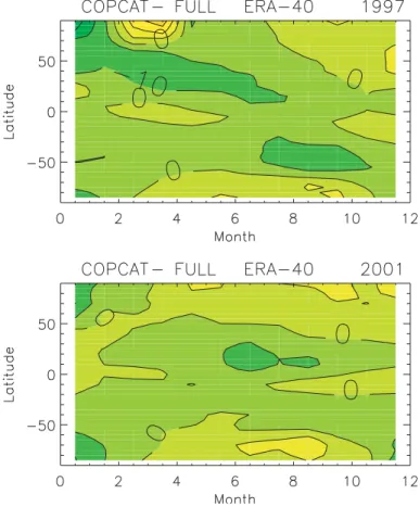
temperatures reached during winter. Year 2000 exhibited a very cold Arctic winter, thus, it is important to evaluate how sensitive the coe_fficients are to the initial calculation con-ditions and to what extent COPCAT is able to generalise its performance to different atmospheric conditions. Figure 10 shows the total column di_fferences between the COPCAT and the full chemistry ozone fields for the years 1997 (cold winter, although

15

warmer than 2000) and 2001 (warm winter). For 1997 (upper panel in Fig. 10) the differences are similar to those in 2001 (0–10 DU), except in the Arctic winter, where COPCAT TO column is over 30 DU larger than the full chemistry. Other cold winters like 2000 (Fig. 5) or 1996 (not shown) exhibit similar patterns in the TO column differences. In 2001 (bottom panel in Fig. 10) differences are small in all months and regions. In

20

the tropical and mid-latitude regions COPCAT columns are 0–10 DU smaller than in the full-chemistry, over high latitudes the parameterisation gives larger column values than the full chemistry, but in no case are these differences larger than 10 DU. This sit-uation is representative of what happens in other warm winters, e.g. 1992 or 1994 (not shown), while for 1999 (warm winter) the Arctic column values are up to 40 DU lower

25

(17)

ACPD

10, 12993–13027, 2010

CTM

Title Page

Tables Figures

◭ ◮

Back Close

Full Screen / Esc

Discussion

P

a

per

|

Dis

cussion

P

a

per

|

Discussion

P

a

per

|

Discussio

n

P

a

per

|

than the full chemistry).

Vertical profiles at 84◦_{N are shown in Fig. 11 for January–July 1997 and 2001. It}

can clearly be seen how COPCAT is able to follow well the full-chemistry variations in both years. For the cold winter COPCAT shows a small underestimation in the middle stratosphere with respect to the full chemistry run, while for the warm winter

5

the agreement is very good at least up to 10 hPa. The ECMWF v2.9 scheme however, tends to underestimate O₃concentrations in the LS (∼0.25 ppmv3) and to overestimate

concentrations above 60 hPa by up to 2 ppmv, the overestimation being more obvious during the early months of winter (January–February). While these di_fferences with the full chemistry are common to both the cold and warm winters, overall the ECMWF

10

scheme is closer to the full chemistry profile during warm winter conditions.

Even if warm and cold winter conditions do not a_ffect the Antarctic as much as the Arctic it is also interesting to check the ability of COPCAT to simulate Antarctic O₃ loss for conditions di_fferent from year 2000. Figure 12 represents the O₃ verti-cal profiles from the COPCAT run, together with the full-chemistry and the ECMWF

15

scheme, for July–December 2001 at 84◦S. These profiles show very clearly the ability of COPCAT to follow the full-chemistry field, while the ECMWF scheme overestimation is also present in this case (above 60 hPa in July–September) and in the LS region in September–December. The spring O₃ hole simulated by COPCAT is in very good agreement with full-chemistry SLIMCAT, while the ECMWF scheme does not deplete

20

as much ozone in the LS region.

5 Summary

This work has tested the current ECMWF O₃parameterisation in a 3-D CTM, and sug-gested improvements for the current operational scheme. An alternative scheme has been proposed here, based on the same CD linear approach, but using a new

calcula-25

3

(18)

ACPD

10, 12993–13027, 2010

CTM

Title Page

Tables Figures

◭ ◮

Back Close

Full Screen / Esc

Discussion

P

a

per

|

Dis

cussion

P

a

per

|

Discussion

P

a

per

|

Discussio

n

P

a

per

tion approach with a consistent treatment of heterogeneous and gas-phase chemistry. For this, the new O₃parameterisation scheme (COPCAT) has been developed with im-plicit heterogeneous chemistry. This novel approach has been presented as a suitable improvement for schemes based on the linear Cariolle and D ´equ ´e approach, such as the operational ECMWF scheme.

5

The new linear ozone scheme has been obtained from SLIMCAT full-chemistry runs and for the first time it has been possible to compare a scheme of this kind with the full chemistry 3-D CTM used to calculate it. This has allowed the isolation of chemistry di_fferences from other factors, such as numerics, resolution or transport. Obtaining a parameterisation based on a widely tested CTM like SLIMCAT is crucial to evaluate

10

and understand di_fferences between the parameterisation and full-chemistry models. Moreover, the approach adopted here ensures that the parameterisation obtained is as close as possible to a state-of-the-art full-chemistry CTM. COPCAT is in good overall agreement with SLIMCAT full-chemistry, although a significant reduction in the tropical maximum O₃ at 10 hPa occurs when using the parameterisation. A similar reduction

15

takes place when using the ECMWF scheme in a SLIMCAT run, which identifies a drawback of this kind of scheme with respect to full-chemistry models. Results have also shown the relevance of the choice of the reference state (climatology); using the Fortuin and Kelder (1998) O₃climatology the tropical differences against observations have been reduced for COPCAT runs.

20

The heterogeneous treatment adopted by COPCAT has provided the scheme with a realistic polar loss simulation showing that the linearisation approach can cope ade-quately with polar chemical processes. The new scheme is able to reproduce a realistic Antarctic ozone hole, and also over northern high latitudes COPCAT is more realistic than the current ECMWF scheme. Both treatments involve approximations, however,

25

(19)

ACPD

10, 12993–13027, 2010

CTM

Title Page

Tables Figures

◭ ◮

Back Close

Full Screen / Esc

Discussion

P

a

per

|

Dis

cussion

P

a

per

|

Discussion

P

a

per

|

Discussio

n

P

a

per

|

Sect. 4.3 COPCAT is able to reproduce the behaviour of the full chemistry model in the Arctic for both warm and cold winters. The adaptability of the scheme makes it a good candidate to be used in the production of a long reanalysis series. Coefficients would only have to be recomputed for periods in which atmospheric chemistry conditions were very di_fferent from present ones, mainly in terms of ozone depleting substances (ODS)

5

concentrations. To adjust the tendencies to the actual chemistry conditions coefficients would be recomputed for years before 1980, when ODS concentrations were still low enough not to produce ozone destruction during the Antarctic spring, and again before the 1960s, when no significant ODS concentrations were present in the atmosphere (WMO, 2007).

10

The inclusion of heterogeneous chemistry in the scheme has not been detrimental for the linearity of the approach. Only at polar latitudes is the range of temperatures for the linear approximation somewhat restricted. Such temperature range (±10 K from

the reference state) is still within the typical variation range observed in global mod-els (e.g. Shine et al., 2003), however, to ensure the accuracy of the scheme under

15

all possible polar vortex conditions higher order terms could be included as a future improvement to the scheme. This would not increase much the cost of the scheme, as it would only mean the coe_fficients files to be read-in would contain more data. Other improvements that can easily be implemented in future COPCAT versions are the use of a higher vertical resolution, as well as basing the scheme in a full-chemistry run

20

using the recent ERA-Interim reanalyses, which have already shown to provide more realistic results in the stratosphere than ERA-40 (e.g. Monge-Sanz et al., 2007). Solar cycle influences could also be included in next COPCAT versions. Moreover, as the full chemistry SLIMCAT model is continuously subject to revisions and improvements, following versions of COPCAT would benefit from the same developments included in

25

the CTM.

(20)

ACPD

10, 12993–13027, 2010

CTM

Title Page

Tables Figures

◭ ◮

Back Close

Full Screen / Esc

Discussion

P

a

per

|

Dis

cussion

P

a

per

|

Discussion

P

a

per

|

Discussio

n

P

a

per

in this study could be applied by any other 3-D CTM with complete ozone chemistry. Deriving this kind of implicitly consistent linear scheme from di_fferent CTMs, and being able to compare with the corresponding full-chemistry model, would add valuable in-formation on the performance of linear O₃parameterisations widely used in NWP and data assimilation systems, such as those of UK Met-O_ffice, ECMWF or M ´et ´eo-France.

5

Acknowledgements. Authors are very grateful to Adrian Simmons for useful discussions and

support throughout this work. We also thank John McCormack for providing the CHEM2D coef-ficients and Agathe Untch, Elias H ´olm and Rossana Dragani for many valuable communications on the ECMWF O3scheme. This work has been partially funded by the NERC Research Award

NE/F004575/1. 10

References

Br ¨uhl, C., Drayson, S. R., Russell III, J. M., Crutzen, P. J., Mclnerney, J. M., Purcell, P. N., Claude, H., Gernandt, H., McGee, T. J., McDermid, I. S., and Gunson, M. R.: Halogen Occultation Experiment ozone channel validation, J. Geophys. Res., 101, 10217–10240, 1996. 13003

15

Cariolle, D. and D ´equ ´e, M.: Southern Hemisphere Medium-Scale Waves and Total Ozone Disturbances in a Spectral General Circulation Model, J. Geophys. Res., 91, 10825–10846, 1986. 12995, 13001

Cariolle, D. and Teyss `edre, H.: A revised linear ozone photochemistry parameterization for use in transport and general circulation models: multi-annual simulations, Atmos. Chem. Phys., 20

7, 2183–2196, doi:10.5194/acp-7-2183-2007, 2007. 12995, 12996, 12998

Carslaw, K. S., Luo, B. P., Clegg, S. L., Peter, T., Brimblecombe, P., and Crutzen, P. J.: Strato-spheric aerosol growth and HNO3gas phase depletion from coupled HNO3and water uptake

by liquid particles, Geophys. Res. Lett., 21, 2479–2482, 1994. 12997

Chipperfield, M. P.: Multiannual simulations with a three-dimensional chemical transport model, 25

J. Geophys. Res., 104, 1781–1805, 1999. 13004

(21)

ACPD

10, 12993–13027, 2010

CTM

Title Page

Tables Figures

◭ ◮

Back Close

Full Screen / Esc

Discussion

P

a

per

|

Dis

cussion

P

a

per

|

Discussion

P

a

per

|

Discussio

n

P

a

per

|

Chipperfield, M. P.: New version of the TOMCAT/SLIMCAT off-line chemical transport model, Q. J. R. Meteorol. Soc., 132, 1179–1203, doi:10.1256/qj.05.51, 2006. 12997, 12999

Chipperfield, M. P., Cariolle, D., and Simon, P.: A 3-Dimensional transport model study of PSC processing during EASOE, Geophys. Res. Lett., 21, 1463–1466, 1994. 12998

Chipperfield, M. P., Khattatov, B. V., and Lary, D. J.: Sequential assimilation of stratospheric 5

chemical observations in a three-dimensional model, J. Geophys. Res., 107(D21), 4585, doi:10.1029/2002JD002110, 2002. 13003

Dethof, A. and H ´olm, E. V.: Ozone assimilation in the ERA-40 reanalysis project, Q. J. R. Meteorol. Soc., 130, 2851–2872, 2004. 12995, 12997, 12998

Eskes, H. J., Van Velthoven, P. F. J., Valks, P. J. M., and Kelder, H. M.: Assimilation of GOME 10

total-ozone satellite observations in a three-dimensional tracer-transport model, Q. J. R. Me-teorol. Soc., 129, 1663–1681, 2003. 12996

Eyring, V., Butchart, N., Waugh, D. W., Akiyoshi, H., Austin, J., Bekki, S., Bodeker, G. E., Boville, B. A., Br ¨uhl, C., Chipperfield, M. P., Cordero, E., Dameris, M., Deushi, M., Fioletov, V. E., Frith, S. M., Garcia, R. R., Gettelman, A., Giorgetta, M. A., Grewe, V., Jourdain, L., Kinnison, 15

D. E., Mancini, E., Manzini, E., Marchand, M., Marsh, D. R., Nagashima, T., Newman, P. A., Nielsen, J. E., Pawson, S., Pitari, G., Plummer, D. A., Rozanov, E., Schraner, M., Shepherd, T. G., Shibata, K., Stolarski, R. S., Struthers, H., Tian, W., and Yoshiki, M.: Assessment of temperature, trace species, and ozone in chemistry-climate model simulations of the recent past, J. Geophys. Res., 111, D22308, doi:10.1029/2006JD007327, 2006. 13003

20

Feng, W., Chipperfield, M. P., Dorf, M., Pfeilsticker, K., and Ricaud, P.: Mid-latitude ozone changes: studies with a 3-D CTM forced by ERA-40 analyses, Atmos. Chem. Phys., 7, 2357–2369, doi:10.5194/acp-7-2357-2007, 2007. 13003

Fortuin, J. P. F. and Kelder, H.: An ozone climatology based on ozonesonde and satellite mea-surements, J. Geophys. Res., 103, 31709–31734, 1998. 13005, 13010, 13022

25

Geer, A. J., Lahoz, W. A., Jackson, D. R., Cariolle, D., and McCormack, J. P.: Evaluation of lin-ear ozone photochemistry parametrizations in a stratosphere-troposphere data assimilation system, Atmos. Chem. Phys., 7, 939–959, doi:10.5194/acp-7-939-2007, 2007. 12996 Hanson, D. and Mauersberger, K.: Laboratory studies of the nitric acid trihydrate: Implications

for the South Polar stratosphere, Geophys. Res. Lett., 15, 855–858, 1988. 12997 30

(22)

ACPD

10, 12993–13027, 2010

CTM

Title Page

Tables Figures

◭ ◮

Back Close

Full Screen / Esc

Discussion

P

a

per

|

Dis

cussion

P

a

per

|

Discussion

P

a

per

|

Discussio

n

P

a

per

Phys., 4, 2401–2423, doi:10.5194/acp-4-2401-2004, 2004. 12996

McCormack, J. P., Eckermann, S. D., Siskind, D. E., and McGee, T. J.: CHEM2D-OPP: A new linearized gas-phase ozone photochemistry parameterization for high-altitude NWP and climate models, Atmos. Chem. Phys., 6, 4943–4972, doi:10.5194/acp-6-4943-2006, 2006. 12995, 12996, 13001

5

McLinden, C. A., Olsen, S. C., Hannegan, B., Wild, O., and Prather, M. J.: Stratospheric Ozone in 3-D Models: A simple chemistry and the cross-tropopause flux, J. Geophys. Res., 105, 14635–14665, 2000. 12995, 12996, 13000, 13001

McPeters, R., Bhartia, P., Krueger, A., Herman, J. R., Wellemeyer, C., Seftor, C., Jaross, G., Torres, O., Moy, L., Labow, G., Byerly, W., Taylor, S., Swissler, T., and Cebula, R.: Earth 10

Probe Total Ozone Mapping Spectrometer (TOMS) Data Products User’s Guide, NASA Ref. Publ. 206895, 1998. 13003

Monge-Sanz, B. M.: Stratospheric Transport and Chemical Parameterisations in ECMWF Anal-yses: Evaluation and Improvements using a 3-D CTM, Ph.D. thesis, Earth and Environment School, University of Leeds, 2008. 12997, 13000, 13004

15

Monge-Sanz, B. M., Chipperfield, M. P., Simmons, A. J., and Uppala, S. M.: Mean age of air and transport in a CTM: Comparison of different ECMWF analyses, Geophys. Res. Lett., 34, L04801, doi:10.1029/2006GL028515, 2007. 13011

Searle, K. R., Chipperfield, M. P., Bekki, S., and Pyle, J. A.: The impact of spatial averaging on calculated polar ozone loss 2. Theoretical analysis, J. Geophys. Res., 103, 25409–25416, 20

1998. 12998

Shine, K. P., Bourqui, M. S., de F. Forster, P. M., Hare, S. H. E., Langematz, U., Braesicke, P., Grewe, V., Ponater, M., Schnadt, C., Smith, C. A., Haigh, J. D., Austin, J., Butchart, N., Shindell, D. T., Randel, W. J., Nagashima, T., Portmann, R. W., Solomon, S., Seidel, D. J., Lanzante, J., Klein, S., Ramaswamy, V., and Schwarzkopf, M. D.: A comparison of model-25

simulated trends in stratospheric temperatures, Q. J. R. Meteorol. Soc., 129, 1565–1588, doi:10.1256/qj.02.186, 2003. 13011

Steil, B., Br ¨uhl, C., Manzini, E., Crutzen, P. J., Lelieveld, J., Rasch, P. J., Roeckner, E., , and Kr ¨uger, K.: A new interactive chemistry-climate model: 1. Present-day climatology and inter-annual variability of the middle atmosphere using the model and 9 years of HALOE/UARS 30

data, J. Geophys. Res., 108(D9), 4290, doi:10.1029/2002JD002971, 2003. 13003

(23)

ACPD

10, 12993–13027, 2010

CTM

Title Page

Tables Figures

◭ ◮

Back Close

Full Screen / Esc

Discussion

P

a

per

|

Dis

cussion

P

a

per

|

Discussion

P

a

per

|

Discussio

n

P

a

per

|

N., Allan, R. P., Andersson, E., Arpe, K., Balmaseda, M. A., Beljaars, A. C. M., Berg, L. V. D., Bidlot, J., Bormann, N., Caires, S., Chevallier, F., Dethof, A., Dragosavac, M., Fisher, M., Fuentes, M., Hagemann, S., H ´olm, E., Hoskins, B. J., Isaksen, L., Janssen, P. A. E. M., Jenne, R., Mcnally, A. P., Mahfouf, J.-F., Morcrette, J.-J., Rayner, N. A., Saunders, R. W., Simon, P., Sterl, A., Trenberth, K. E., Untch, A., Vasiljevic, D., Viterbo, P., and Woollen, J.: 5

The ERA-40 Re-analysis, Q. J. R. Meteorol. Soc., 131, 2961–3012, doi:10.1256/qj.04.176, 2005. 13000

WMO: Scientific Assessment of Ozone Depletion: 2006, Global Ozone Research and Monitor-ing Project -Report No. 50, WMO (World Meteorological Organization), Geneva, Switzerland, 2007. 13011

(24)

ACPD

10, 12993–13027, 2010

CTM

Title Page

Tables Figures

◭ ◮

Back Close

Full Screen / Esc

Discussion

P

a

per

|

Dis

cussion

P

a

per

|

Discussion

P

a

per

|

Discussio

n

P

a

per

a) (P-L)0 SEP

COPCAT

b) (P-L)0 SEP

Cariolle v2.9

c) (P-L)0 SEP

LINOZ

d) (P-L)0 SEP

CHEM2D

(25)

ACPD

10, 12993–13027, 2010

CTM

Title Page

Tables Figures

◭ ◮

Back Close

Full Screen / Esc

Discussion

P

a

per

|

Dis

cussion

P

a

per

|

Discussion

P

a

per

|

Discussio

n

P

a

per

|

a) (P-L)0 JUN COPCAT

b) (P-L)0 JUL COPCAT

c) (P-L)0 AUG COPCAT

d) (P-L)0 SEP COPCAT

Fig. 2.Altitude/latitude distribution of COPCAT net ozone productionc₀_{(see text in Sect. 1 for}

(26)

ACPD

10, 12993–13027, 2010

CTM

Title Page

Tables Figures

◭ ◮

Back Close

Full Screen / Esc

Discussion

P

a

per

|

Dis

cussion

P

a

per

|

Discussion

P

a

per

|

Discussio

n

P

a

per

a) b)

85 hPa 11 hPa 3 hPa

c)

Fig. 3. COPCAT (P-L) values as a function of the perturbation in(a) temperatureT, (b)local ozonef and(c)column abovec_O

3, at 40

◦_{N in May. Pressure levels shown are 85 hPa (black),} 11 hPa (blue) and 3 hPa (red). Solid lines correspond to the exact tendencies from the box model; dashed lines correspond to the least squares fit for the perturbation values used for COPCAT coefficients (Sect. 2). To show all results within the same vertical axis, those for the 3 hPa level have been scaled by 0.1, 0.25 and 0.1 forT_,f _andc_O

(27)

ACPD

10, 12993–13027, 2010

CTM

Title Page

Tables Figures

◭ ◮

Back Close

Full Screen / Esc

Discussion

P

a

per

|

Dis

cussion

P

a

per

|

Discussion

P

a

per

|

Discussio

n

P

a

per

|

a) _b)

85 hPa 111 hPa

52 hPa c)

(28)

ACPD

10, 12993–13027, 2010

CTM

Title Page

Tables Figures

◭ ◮

Back Close

Full Screen / Esc

Discussion

P

a

per

|

Dis

cussion

P

a

per

|

Discussion

P

a

per

|

Discussio

n

P

a

per

a)

b)

(29)

ACPD

10, 12993–13027, 2010

CTM

Title Page

Tables Figures

◭ ◮

Back Close

Full Screen / Esc

Discussion

P

a

per

|

Dis

cussion

P

a

per

|

Discussion

P

a

per

|

Discussio

n

P

a

per

|

84ºN

84ºS

(30)

ACPD

10, 12993–13027, 2010

CTM

Title Page

Tables Figures

◭ ◮

Back Close

Full Screen / Esc

Discussion

P

a

per

|

Dis

cussion

P

a

per

|

Discussion

P

a

per

|

Discussio

n

P

a

per

4ºN

fk fk

Fig. 7.Annual average 2000 O3(ppmv) profile at 4◦N from SLIMCAT runs using the COPCAT

(31)

ACPD

10, 12993–13027, 2010

CTM

Title Page

Tables Figures

◭ ◮

Back Close

Full Screen / Esc

Discussion

P

a

per

|

Dis

cussion

P

a

per

|

Discussion

P

a

per

|

Discussio

n

P

a

per

|

c) b) a)

0

10 20

30

40

50

60

70 80

0 20

0 -10

-20

-30

0

-10

-20

20 -20

50

0

-10

20 70 -10

-30

60

20

1030 0 50

Fig. 8. Total O3 column differences (DU) with respect to TOMS for SLIMCAT runs using(a)

(32)

ACPD

10, 12993–13027, 2010

CTM

Title Page

Tables Figures

◭ ◮

Back Close

Full Screen / Esc

Discussion

P

a

per

|

Dis

cussion

P

a

per

|

Discussion

P

a

per

|

Discussio

n

P

a

per

a)

c)

b)

d)

85ºS 75ºS

85ºN 75ºN

column (DU)

Fig. 9.Total ozone column (DU) zonally averaged time series January–December 2000 at(a) 85◦_N,

(b) 75◦_N,

(c) 85◦_{S and}

(33)

ACPD

10, 12993–13027, 2010

CTM

Title Page

Tables Figures

◭ ◮

Back Close

Full Screen / Esc

Discussion

P

a

per

|

Dis

cussion

P

a

per

|

Discussion

P

a

per

|

Discussio

n

P

a

per

|

(34)

ACPD

10, 12993–13027, 2010

CTM

Title Page

Tables Figures

◭ ◮

Back Close

Full Screen / Esc

Discussion

P

a

per

|

Dis

cussion

P

a

per

|

Discussion

P

a

per

|

Discussio

n

P

a

per

84ºN 1997

84ºN 2001

(35)

ACPD

10, 12993–13027, 2010

CTM

Title Page

Tables Figures

◭ ◮

Back Close

Full Screen / Esc

Discussion

P

a

per

|

Dis

cussion

P

a

per

|

Discussion

P

a

per

|

Discussio

n

P

a

per

|

84ºS

2001