ACPD
15, 5849–5957, 2015Global OZone Chemistry And Related Datasets for
the Stratosphere (GOZCARDS)
L. Froidevaux et al.
Title Page
Abstract Introduction
Conclusions References
Tables Figures
◭ ◮
◭ ◮
Back Close
Full Screen / Esc
Printer-friendly Version
Interactive Discussion
Discussion
P
a
per
|
Discussion
P
a
per
|
Discussion
P
a
per
|
Discussion
P
a
per
|
Atmos. Chem. Phys. Discuss., 15, 5849–5957, 2015 www.atmos-chem-phys-discuss.net/15/5849/2015/ doi:10.5194/acpd-15-5849-2015
© Author(s) 2015. CC Attribution 3.0 License.
This discussion paper is/has been under review for the journal Atmospheric Chemistry and Physics (ACP). Please refer to the corresponding final paper in ACP if available.
Global OZone Chemistry And Related
Datasets for the Stratosphere
(GOZCARDS): methodology and sample
results with a focus on HCl, H
2
O, and O
3
L. Froidevaux1, J. Anderson2, H.-J. Wang3, R. A. Fuller1, M. J. Schwartz1, M. L. Santee1, N. J. Livesey1, H. C. Pumphrey4, P. F. Bernath5, J. M. Russell III2,
and M. P. McCormick2
1
Jet Propulsion Laboratory, California Institute of Technology, Pasadena, CA, USA
2
Hampton University, Hampton, VA, USA
3
Georgia Institute of Technology, Atlanta, GA, USA
4
The University of Edinburgh, Edinburgh, UK
5
Old Dominion University, Norfolk, VA, USA
Received: 5 December 2014 – Accepted: 3 February 2015 – Published: 2 March 2015
Correspondence to: L. Froidevaux ([email protected])
ACPD
15, 5849–5957, 2015Global OZone Chemistry And Related Datasets for
the Stratosphere (GOZCARDS)
L. Froidevaux et al.
Title Page
Abstract Introduction
Conclusions References
Tables Figures
◭ ◮
◭ ◮
Back Close
Full Screen / Esc
Printer-friendly Version
Interactive Discussion
Discussion
P
a
per
|
Discussion
P
a
per
|
Discussion
P
a
per
|
Discussion
P
a
per
|
Abstract
We describe the publicly available dataset from the Global OZone Chemistry And Re-lated Datasets for the Stratosphere (GOZCARDS) project, and provide some results, with a focus on hydrogen chloride (HCl), water vapor (H2O), and ozone (O3). This dataset is a global long-term stratospheric Earth System Data Record (ESDR),
con-5
sisting of monthly zonal mean time series starting as early as 1979. The data records are based on high quality measurements from several NASA satellite instruments and ACE-FTS on SCISAT. We examine consistency aspects between the various datasets. To merge ozone records, the time series are debiased by calculating average offsets with respect to SAGE II during periods of measurement overlap, whereas for other
10
species, the merging derives from an averaging procedure based on overlap periods. The GOZCARDS files contain mixing ratios on a common pressure/latitude grid, as well as standard errors and other diagnostics; we also present estimates of systematic un-certainties in the merged products. Monthly mean temperatures for GOZCARDS were also produced, based directly on data from the Modern-Era Retrospective analysis for
15
Research and Applications (MERRA).
The GOZCARDS HCl merged product comes from HALOE, ACE-FTS and (for the lower stratosphere) Aura MLS data. After a rapid rise in upper stratospheric HCl in the early 1990s, the rate of decrease in this region for 1997–2010 was between 0.4 and 0.7 % yr−1. On shorter timescales (6 to 8 years), the rate of decrease peaked in
20
2004–2005 at about 1 % yr−1, and has since levelled off, at ∼0.5 % yr−1. With a delay of 6–7 years, these changes roughly follow total surface chlorine, whose behavior vs. time arises from inhomogeneous changes in the source gases. Since the late 1990s, HCl decreases in the lower stratosphere have occurred with pronounced latitudinal variability at rates sometimes exceeding 1–2 % yr−1. There has been a significant
re-25
ACPD
15, 5849–5957, 2015Global OZone Chemistry And Related Datasets for
the Stratosphere (GOZCARDS)
L. Froidevaux et al.
Title Page
Abstract Introduction
Conclusions References
Tables Figures
◭ ◮
◭ ◮
Back Close
Full Screen / Esc
Printer-friendly Version
Interactive Discussion
Discussion
P
a
per
|
Discussion
P
a
per
|
Discussion
P
a
per
|
Discussion
P
a
per
|
reversing after about 2011, with (short-term) decreases at northern midlatitudes and some increasing tendencies at southern midlatitudes.
For GOZCARDS H2O, covering the stratosphere and mesosphere, the same
instru-ments as for HCl are used, along with UARS MLS stratospheric H2O data (1991–1993). We display seasonal to decadal-type variability in H2O from 22 years of data. In the up-5
per mesosphere, the anti-correlation between H2O and solar flux is now clearly visible
over two full solar cycles. Lower stratospheric tropical H2O has exhibited two periods of increasing values, followed by fairly sharp drops, the well-documented 2000–2001 de-crease, and another recent decrease in 2011–2013. Tropical decadal variability peaks just above the tropopause. Between 1991 and 2013, both in the tropics and on a
near-10
global basis, H2O has decreased by ∼5–10 % in the lower stratosphere, but about
a 10 % increase is observed in the upper stratosphere and lower mesosphere. How-ever, recent tendencies may not hold for the long-term, and the addition of a few years of data can significantly modify trend results.
For ozone, we used SAGE I, SAGE II, HALOE, UARS and Aura MLS, and ACE-FTS
15
data to produce a merged record from late 1979 onward, using SAGE II as the primary reference for aligning (debiasing) the other datasets. Other adjustments were needed in the upper stratosphere to circumvent temporal drifts in SAGE II O3after June 2000,
as a result of the (temperature-dependent) data conversion from a density/altitude to a mixing ratio/pressure grid. Unlike the 2 to 3 % increase in near-global column ozone
20
after the late 1990s reported by some, GOZCARDS stratospheric column O3 values
do not show a recent upturn of more than 0.5 to 1 %; continuing studies of changes in global ozone profiles, as well as ozone columns, are warranted.
A brief mention is also made of other currently available, commonly-formatted GOZ-CARDS satellite data records for stratospheric composition, namely those for N2O and 25
ACPD
15, 5849–5957, 2015Global OZone Chemistry And Related Datasets for
the Stratosphere (GOZCARDS)
L. Froidevaux et al.
Title Page
Abstract Introduction
Conclusions References
Tables Figures
◭ ◮
◭ ◮
Back Close
Full Screen / Esc
Printer-friendly Version
Interactive Discussion
Discussion
P
a
per
|
Discussion
P
a
per
|
Discussion
P
a
per
|
Discussion
P
a
per
|
1 Introduction
The negative impact of anthropogenic chlorofluorocarbon emissions on the ozone layer, following the early predictions of Molina and Rowland (1974), stimulated interest in the trends and variability of stratospheric ozone, a key absorber of harmful ultraviolet radiation. The discovery of the ozone hole in ground-based data records (Farman et al.,
5
1985) and the associated dramatic ozone changes during Southern Hemisphere winter and spring raised the level of research and understanding regarding the existence of new photochemical processes (see Solomon, 1999). This research was corroborated by analyses of aircraft and satellite datasets (e.g., Anderson et al., 1989; Waters et al., 1993), and by independent ground-based data. Global total column ozone averages in
10
2006–2009 were measured to be smaller than during 1964–1980 by∼3 %, and larger more localized decreases over the same periods reached∼6 % in the Southern Hemi-sphere midlatitudes (WMO, 2011). Halogen source gas emissions have continued to decrease as a result of the Montreal Protocol and its amendments. Surface loading of total chlorine peaked in the early 1990s (WMO, 2011), and subsequent decreases in
15
global stratospheric HCl and ClO have been measured from satellite-based sensors (Anderson et al., 2000; Froidevaux et al., 2006; Jones et al., 2011) as well as from the ground (e.g., Solomon et al., 2006; Kohlhepp et al., 2012). A slow recovery of the ozone layer is expected between the late 1990s and several decades from now, to-wards pre-1985 levels (WMO, 2011); the robust determination of a long-term global
20
trend requires a sufficiently long and accurate data record. It is desirable to use high quality datasets for ozone and related stratospheric species for a robust documentation of past variations and as constraints for global atmospheric models.
The history of global stratospheric observations includes a large suite of satellite-based instruments, generally well-suited for the elucidation of long-term global change.
25
ACPD
15, 5849–5957, 2015Global OZone Chemistry And Related Datasets for
the Stratosphere (GOZCARDS)
L. Froidevaux et al.
Title Page
Abstract Introduction
Conclusions References
Tables Figures
◭ ◮
◭ ◮
Back Close
Full Screen / Esc
Printer-friendly Version
Interactive Discussion
Discussion
P
a
per
|
Discussion
P
a
per
|
Discussion
P
a
per
|
Discussion
P
a
per
|
vapor and ozone intercomparisons have been published by Hegglin et al. (2013) and Tegtmeier et al. (2013), respectively, to be followed by a larger report on intercom-parisons of multiple species. Systematic biases reported in these recent papers tend to mirror past validation work. However, these investigations have not pursued data merging aspects or the creation of long-term records.
5
Under the Global OZone Chemistry And Related Datasets for the Stratosphere (GOZCARDS) project, we have created monthly zonally averaged datasets of strato-spheric composition on a common latitude/pressure grid, using satellite-based limb viewing instruments launched as early as 1979 (for ozone data in particular) and now continuing with instruments launched about a decade ago. The creation of this Earth
10
System Data Record stays close to the data values themselves. Therefore, spatial or temporal gaps are typically not filled in; various methods can be used to try to produce continuous fits to time series, but we viewed this as being outside the scope of this data record creation. The GOZCARDS products arise from several high quality satellite datasets, namely from Stratospheric Aerosol and Gas Experiment instruments (SAGE
15
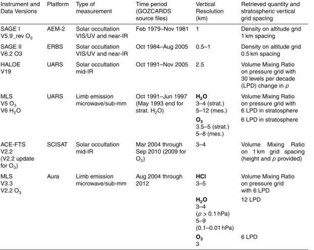
I and SAGE II), the Halogen Occultation Experiment (HALOE) which flew aboard the Upper Atmosphere Research Satellite (UARS), the UARS Microwave Limb Sounder (MLS), the Atmospheric Chemistry Experiment Fourier Transform Spectrometer (ACE-FTS) on SCISAT, and the Aura MLS experiment. Table 1 provides characteristics of the original datasets; validation papers from the instrument teams and other related
stud-20
ies give a certain degree of confidence in these datasets. However, the existence of validation references does not imply that there are no caveats or issues with a particu-lar measurement suite. In this project, we have strived to optimize data screening and mitigate some undesirable features, such as the impact of outlier values or the effects of clouds or aerosols. All source datasets still have shortcomings or imperfections, but
25
we have refrained from arbitrarily removing specific monthly means.
fol-ACPD
15, 5849–5957, 2015Global OZone Chemistry And Related Datasets for
the Stratosphere (GOZCARDS)
L. Froidevaux et al.
Title Page
Abstract Introduction
Conclusions References
Tables Figures
◭ ◮
◭ ◮
Back Close
Full Screen / Esc
Printer-friendly Version
Interactive Discussion
Discussion
P
a
per
|
Discussion
P
a
per
|
Discussion
P
a
per
|
Discussion
P
a
per
|
lowed by binning and averaging into monthly sets. In order to accomodate the lower vertical resolution of some limb viewers, such as UARS MLS, the GOZCARDS pres-sure grid was chosen as
p(i)=1000×10−i /6(hPa) (1)
with i varying from 0 to a product-dependent top; this grid width corresponds to
5
∼2.7 km. The high resolution SAGE O3 profiles were smoothed vertically onto this
grid (see Sect. 5). Given the sampling of solar occultation instruments, which typically provide 15 sunrise (SR) and 15 sunset (SS) profiles every day (vs. the emission-based sampling from MLS), we used latitude bins of width 10◦(18 bins from 80–90◦S to 80– 90◦N) to construct the monthly zonal means.
10
After the production of GOZCARDS source data files on the above grid, merged (combined) products were created. This involves the calculation of average biases be-tween monthly zonal means from different source data during periods of overlap, fol-lowed by an adjustment (using calculated average offsets) of the time series. Non-zero biases always exist between datasets from different instruments for various reasons,
15
such as systematic errors arising from Level 1 (radiances) or Level 2 (retrievals), diff er-ent vertical resolutions, or sampling effects. A useful reference regarding the sampling effects, which can arise spatially (within a latitude bin) or temporally (within a month), is the recent work by Toohey et al. (2013). They studied sampling biases from a large suite of satellite-based stratospheric profiling instruments, based on simulations
us-20
ing fully-sampled model abundance averages vs. averaged sampled results from sub-orbital track locations. The magnitude of such sampling errors is typically inversely related to the number of available profiles routinely sampled, so that larger sampling errors arise from occultation than from emission measurements, which often sample thousands of profiles per day. Toohey et al. (2013) found that sampling-related biases
25
ACPD
15, 5849–5957, 2015Global OZone Chemistry And Related Datasets for
the Stratosphere (GOZCARDS)
L. Froidevaux et al.
Title Page
Abstract Introduction
Conclusions References
Tables Figures
◭ ◮
◭ ◮
Back Close
Full Screen / Esc
Printer-friendly Version
Interactive Discussion
Discussion
P
a
per
|
Discussion
P
a
per
|
Discussion
P
a
per
|
Discussion
P
a
per
|
We have observed very good correlations between GOZCARDS ozone and other long-term ozone datasets, such as the Stratospheric Water vapor and OzOne Satel-lite Homogenized (SWOOSH) dataset (Davis et al., personal communication, 2012) and homogenized Solar Backscatter Ultraviolet (SBUV) data; these analyses (along with related work on H2O) will be discussed elsewhere. Results from GOZCARDS and 5
other data relating to midlatitude ozone trends have appeared (e.g., Nair et al., 2013). Dissemination of trend results arising from analyses of GOZCARDS and other ozone profile data is planned as part of the SI2N initiative, which stands for Stratospheric Pro-cesses And their Role in Climate (SPARC), International Ozone Commission (IOC), Integrated Global Atmospheric Chemistry Observations (IGACO-O3), and the Network
10
for the Detection of Atmospheric Composition Change (NDACC). Recent results on such ozone profile trend comparisons can be found in Tummon et al. (2014) and Harris et al. (2015).
This paper starts with a discussion of general data screening issues (Sect. 2), and then describes the GOZCARDS data production approach and methodology, followed
15
by some atmospheric results for HCl (Sect. 3), H2O (Sect. 4), and O3 (Sect. 5). We
provide specific diagnostics that indicate generally good correlations and small relative drifts between the main datasets being used to create the longer-term GOZCARDS merged time series. Section 6 briefly mentions the availability of a few other GOZ-CARDS products, namely N2O, HNO3, and temperatures derived from MERRA fields.
20
The version of GOZCARDS described here is referred to as ESDR version 1.01 or ev1.01. Each product’s public GOZCARDS data record has an associated digital ob-ject identifier (DOI) along with a relevant dataset reference.
2 GOZCARDS source data and data screening
Data provenance information regarding the various measurements used as inputs for
25
ACPD
15, 5849–5957, 2015Global OZone Chemistry And Related Datasets for
the Stratosphere (GOZCARDS)
L. Froidevaux et al.
Title Page
Abstract Introduction
Conclusions References
Tables Figures
◭ ◮
◭ ◮
Back Close
Full Screen / Esc
Printer-friendly Version
Interactive Discussion
Discussion
P
a
per
|
Discussion
P
a
per
|
Discussion
P
a
per
|
Discussion
P
a
per
|
2.1 GOZCARDS data screening and binning
The screening of profiles for GOZCARDS has largely followed guidelines recom-mended by the various instrument teams and/or relevant publications; such screening procedures are rarely all described in one convenient location, so we review this briefly here for the various data sets. Data screening can reduce the total number of good
pro-5
files below our chosen threshold for flagging zonal monthly means; unless otherwise noted, we only provide monthly means constructed from 15 or more values in a given latitude/pressure bin.
For HALOE, cloud contamination may add retrieval artifacts and HALOE profiles were screened for clouds, following procedures described in Hervig and McHugh
10
(1999); values at and below the cloud level (found in the netCDF files) were excluded. Also, HALOE profiles that may occasionally contain artifacts associated with either a faulty trip angle or constant lockdown angle registration were screened out, per rec-ommendations from the HALOE data processing team (see http://haloe.gats-inc.com/ user_docs/index.php for details).
15
For UARS MLS, we used screening recommendations documented by Livesey et al. (2003). In particular, MLS data points whose retrieved precisions are flagged with a negative sign were discarded, ensuring only a negligible contribution to the re-trieval from a priori. Also, our data filtering followed the recommendations regarding the “MMAF_STAT” flag for operational status (we only used values of “G”, “t”, or “T” for this
20
flag) and the product-specific “QUALITY” flag (for which we only used values equal to 4, thus eliminating bad radiance fits).
For Aura MLS data screening, the procedures are generally as follows: we only use profiles with even values of the Status field, Quality values larger than documented thresholds (indicating good radiance fits), Convergence values smaller than
docu-25
rec-ACPD
15, 5849–5957, 2015Global OZone Chemistry And Related Datasets for
the Stratosphere (GOZCARDS)
L. Froidevaux et al.
Title Page
Abstract Introduction
Conclusions References
Tables Figures
◭ ◮
◭ ◮
Back Close
Full Screen / Esc
Printer-friendly Version
Interactive Discussion
Discussion
P
a
per
|
Discussion
P
a
per
|
Discussion
P
a
per
|
Discussion
P
a
per
|
ommendations, with appropriate flag values for Quality and Convergence; see Livesey et al. (2013) for such references and v3.3 data screening updates.
For ACE-FTS, a list of profiles with data issues is provided by the ACE-FTS team (see https://databace.scisat.ca/validation/data_issues_table.php) and these have been removed from our database. However, we also found it necessary to remove occasional
5
large outlier values that could significantly impact monthly zonal means by adding a bias (or “noise”) to the time series if such screening were not performed; such out-liers are not otherwise routinely removed from the original ACE-FTS profiles. Our outlier screening procedure removed values outside 2.5 times the SD, as measured from the median values in each latitude/pressure bin, for each year of data. This was deemed
10
close to optimum by comparing the results to Aura MLS time series (which usually are not impacted by such outliers), as well as to independent zonal means (using 5◦ lati-tude bins) provided by the ACE-FTS instrument team. Up to 5 % of the profile values in each bin in any given month were typically discarded as a result of this procedure, but the maximum percentage of discarded values can be close to 10 % for a few months of
15
ACE-FTS version 2.2 data, depending on year and species. Moreover, because of poor ACE-FTS sampling in the tropics, the threshold value for minimum number of (good) ACE-FTS profiles determining a monthly zonal average was allowed to be as low as 10 for mid- to high latitudes, and as low as 6 for low latitudes (bins centered from 25◦S to 25◦N). Our zonal mean datasets for ACE-FTS would become too sparse in some
20
years if such lower threshold values were not used; such data sparseness can intro-duce limitations (larger error bars) in the determination of trends, for example, although we also performed comparisons vs. Aura MLS monthly means to provide some level of confidence in the results. In addition, ACE-FTS single profile values were discarded if the associated error was larger than the mixing ratio or smaller than 10−4times the
25
mixing ratio, following recommendations from the ACE-FTS team.
ACPD
15, 5849–5957, 2015Global OZone Chemistry And Related Datasets for
the Stratosphere (GOZCARDS)
L. Froidevaux et al.
Title Page
Abstract Introduction
Conclusions References
Tables Figures
◭ ◮
◭ ◮
Back Close
Full Screen / Esc
Printer-friendly Version
Interactive Discussion
Discussion
P
a
per
|
Discussion
P
a
per
|
Discussion
P
a
per
|
Discussion
P
a
per
|
its associated standard error (or a few times this standard error) can in theory be mean-ingful, we deem that occasional small negative monthly means are unlikely to be very useful, scientifically.
The organization of profiles on a common pressure grid is straightforward when pres-sure values are present in the original files, as is the case for most data used here.
5
Also, the vertical resolutions are similar for most of the instruments used for GOZ-CARDS (see more details in each species-specific section). The UARS MLS, HALOE, and Aura MLS native pressure grids are either the same as or a superset of the GOZ-CARDS pressure grid, so these datasets were readily sampled for the construction of the GOZCARDS monthly means. For ACE-FTS profiles, pressures are provided along
10
with the fixed altitude grid, and we used linear interpolation vs. log(pressure) to convert profiles to the GOZCARDS grid. More details are provided in the O3section for SAGE
I and SAGE II, for which density vs. altitude is the native representation.
3 GOZCARDS HCl
3.1 GOZCARDS HCl source data records
15
We used HCl datasets from HALOE, ACE-FTS and Aura MLS to generate the monthly zonal mean source products for GOZCARDS HCl.
For the screening of HALOE HCl profiles, in addition to the procedures mentioned in Sect. 2, a first-order aerosol screening was applied: all HCl values at and below a level where the 5.26 µm aerosol extinction exceeds 10−3km−1were excluded.
20
For Aura MLS, the ongoing standard HCl product is retrieved using band 14 rather than band 13, which was used to measure HCl for the first 1.5 years after launch, but started deteriorating rapidly after February 2006. Validation and error characterization for the Aura MLS HCl product (version 2.2) were provided by Froidevaux et al. (2008). The MLS version 3.3/3.4 HCl data used here (see Livesey et al., 2013) compare quite
25
ACPD
15, 5849–5957, 2015Global OZone Chemistry And Related Datasets for
the Stratosphere (GOZCARDS)
L. Froidevaux et al.
Title Page
Abstract Introduction
Conclusions References
Tables Figures
◭ ◮
◭ ◮
Back Close
Full Screen / Esc
Printer-friendly Version
Interactive Discussion
Discussion
P
a
per
|
Discussion
P
a
per
|
Discussion
P
a
per
|
Discussion
P
a
per
|
HCl vs. aircraft data at 147 hPa at low latitudes (Froidevaux et al., 2008). Such re-gions with large uncertainties and biases are avoided (flagged) for the production of the GOZCARDS merged HCl dataset.
The use of the GOZCARDS source files for Aura MLS HCl, like the use of original Level 2 MLS HCl files, is not recommended for obtaining realistic trends in the upper
5
stratosphere (at pressures<10 hPa), even if monthly mean MLS HCl in this region dis-plays reasonable values in comparison to other satellite-based measurements. Aura MLS switched to a backup band (band 14) to retrieve the daily HCl measurements af-ter band 13 (originally targeted specifically for HCl) showed signs of rapid degradation in early 2006; as the remaining lifetime for band 13 is expected to be very short (days
10
as opposed to weeks), this band has only been turned on for a few days since Febru-ary 2006. However, for pressures≥10 hPa, the long-term (band 14) HCl data now be-ing routinely produced is deemed to be robust (because of the broader emission line in this region, in comparison to the measurement bandwidth). These considerations have implications for how we treat MLS HCl upper stratospheric data in terms of the merging
15
process.
Past validation studies have compared MLS HCl (v2.2), ACE-FTS (v2.2) and HALOE (v19) datasets using coincident pairs of profiles; such work was described by Froide-vaux et al. (2008) for MLS HCl validation and by Mahieu et al. (2008) for ACE-FTS HCl validation. HALOE HCl values were found to be biased low by ∼10–15 % relative to 20
both MLS and ACE-FTS, especially in the upper stratosphere; this low bias vs. other (balloon- and space-based) measurements had been noted in past HALOE validation studies (Russell et al., 1996). Also, HALOE (v19) and ACE-FTS (v2.2) HCl data tend to lose sensitivity and reliability for pressures less than∼0.4 hPa.
3.2 GOZCARDS HCl merged data records
25
ACPD
15, 5849–5957, 2015Global OZone Chemistry And Related Datasets for
the Stratosphere (GOZCARDS)
L. Froidevaux et al.
Title Page
Abstract Introduction
Conclusions References
Tables Figures
◭ ◮
◭ ◮
Back Close
Full Screen / Esc
Printer-friendly Version
Interactive Discussion
Discussion
P
a
per
|
Discussion
P
a
per
|
Discussion
P
a
per
|
Discussion
P
a
per
|
trends, because of the Aura MLS HCl trend detection issue mentioned above. Aura MLS HCl time series were not included in the merging at pressures less than 10 hPa, so after November 2005, the GOZCARDS HCl upper stratospheric trends are dictated only by changes in ACE-FTS abundances. However, in order to derive the systematic offsets needed to adjust the time series from these three instruments in a continuous
5
way (in the pressure dimension), we used the absolute Aura MLS HCl measurements at all pressure levels in 2004 and 2005, during the overlap period between the three instruments.
Figure 1 illustrates the merging process for HCl at 32 hPa for the 45◦S latitude bin (which covers 40 to 50◦S). Given that there exists very little overlap between the three
10
sets of measurements in the same months in 2004 and 2005, especially in the tropics, a simple 3-way averaging of the datasets is not practical and would lead to significant data gaps. Our methodology is equivalent to averaging all three datasets during this period (if one had full coverage from all datasets), but we use Aura MLS as a transfer dataset. This was done by first averaging ACE-FTS and Aura MLS data, where the
15
datasets overlap, and then including the third dataset (HALOE) into the merging pro-cess with the intermediate (temporary) merged data. Although HALOE HCl is believed to be biased too low, modifying the HALOE values to somehow match ACE-FTS or Aura MLS values or a combination of these two datasets was deemed to be too sub-jective. The combined weight of the other two datasets leads to a merged HCl dataset
20
that is generally further away from HALOE than it is from either ACE-FTS or Aura MLS. The top left panel in Fig. 1 shows monthly zonal average GOZCARDS source data for HALOE, ACE-FTS, and Aura MLS during the overlap period, from August 2004 (when Aura MLS data started) through November 2005 (when HALOE data ended). The top right panel illustrates the result of step 1 in the merging procedure, with the
tempo-25
ACPD
15, 5849–5957, 2015Global OZone Chemistry And Related Datasets for
the Stratosphere (GOZCARDS)
L. Froidevaux et al.
Title Page
Abstract Introduction
Conclusions References
Tables Figures
◭ ◮
◭ ◮
Back Close
Full Screen / Esc
Printer-friendly Version
Interactive Discussion
Discussion
P
a
per
|
Discussion
P
a
per
|
Discussion
P
a
per
|
Discussion
P
a
per
|
ACE-FTS obtained monthly data (since Aura MLS HCl means exist every month). The middle left panel shows the result of step 2, namely the merged values (brown) that arise from merging HALOE values with the temporary merged values (orange) from step 1. In this second averaging step, we weigh the intermediate merged values by 2/3 and HALOE values by 1/3 (leading to a mean reference illustrated by the dashed
5
black line), in order for this process to be equivalent to averaging all three datasets, each with a weight of 1/3. The middle right panel shows the source data along with the final merged values during the overlap period. A simple mathematical description of the above procedure is provided in Appendix A. The bottom panel shows the same datasets but for 1991 through 2012, after the calculated additive offsets are applied to
10
the whole source series, thus debiasing the datasets; these adjusted time series are then merged (averaged) together wherever overlap exists. We tested this procedure by using one or the other of the two occultation datasets as the initial one in step 1, and results were not found to differ appreciably. This methodology is used as well for the same three datasets for the H2O merging; we have also checked our procedures and 15
results by using two independent calculations from different institutions. We also found that the use of multiplicative adjustments generally produces very similar results as additive offsets. Some issues were found on occasion with multiplicative offsets, when combining very low mixing ratios, but additive offsets can also have drawbacks if the merged values end up being slightly negative, notably as a result of changes that
mod-20
ify the already low HCl values during Antarctic polar winter. This occurs on occasion as additive offsets tend to be weighted more heavily by the larger mixing ratios found during non-winter seasons; as a result, we decided not to offset the lower stratospheric HCl source datasets in the polar winter seasons at high latitudes for any of the years (for interannual consistency). Procedural details regarding the merging of HCl data are
25
summarized in the Supplement.
ACPD
15, 5849–5957, 2015Global OZone Chemistry And Related Datasets for
the Stratosphere (GOZCARDS)
L. Froidevaux et al.
Title Page
Abstract Introduction
Conclusions References
Tables Figures
◭ ◮
◭ ◮
Back Close
Full Screen / Esc
Printer-friendly Version
Interactive Discussion
Discussion
P
a
per
|
Discussion
P
a
per
|
Discussion
P
a
per
|
Discussion
P
a
per
|
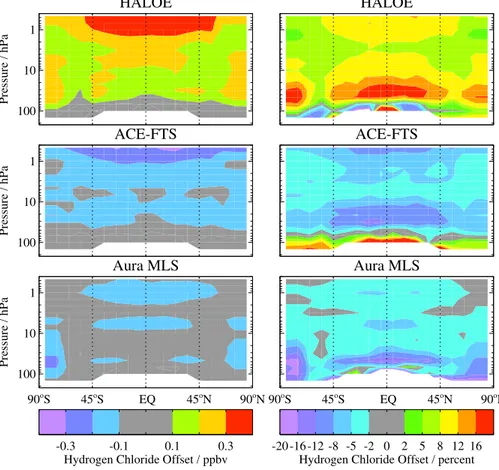
These offsets show that in general, ACE-FTS and Aura MLS HCl values were adjusted down by 0.1–0.2 ppbv (a decrease of about 2–10 %), while HALOE HCl was adjusted upward by 0.2–0.4 ppbv. Offset values tend to be fairly constant with latitude and the sum of the offsets equals zero. The generally homogeneous behaviour vs. latitude is a good sign, as large discontinuities would signal potential issues in the merging (e.g.,
5
arising from large variability or lack of sufficient statistics). Figure S1 provides more detailed examples of some of these (upper and lower stratospheric) offsets vs. latitude, including standard errors based on the variability in the offsets from month to month during the overlap period. Error bars in the offsets provide an indication of the results’ robustness. Another indication of first-order compatibility between datasets is provided
10
by a comparison of annual cycles. Figure S2 provides average annual cycle amplitudes obtained from simple regression model fits to HALOE, ACE-FTS, and Aura MLS series over their respective periods. While there are a few regions where noise or spikes exist (mainly for ACE-FTS), large annual amplitudes in the polar regions occur in all the time series; this arises from HCl decreases in polar winter, followed by springtime increases.
15
A more detailed analysis of interannual variability and trend consistency is provided from results in Fig. 3, which shows an example of ACE-FTS and Aura MLS time series. We note that no v2.2 ACE-FTS data (for any species) are used after September 2010, because of a data processing problem; a fully updated version of ACE-FTS data was not available when the GOZCARDS data records were constructed. We have used
20
coincident points from these time series to compare the deseasonalized anomalies (middle panel in Fig. 3) from both instrument series; correlation coefficient values (R values) are also computed. In the Fig. 3 example, very good correlations are obtained and no significant trend difference between the anomalies (bottom panel) is found for ACE-FTS and Aura MLS HCl. A global view for all latitude/pressure bins of these
cor-25
ACPD
15, 5849–5957, 2015Global OZone Chemistry And Related Datasets for
the Stratosphere (GOZCARDS)
L. Froidevaux et al.
Title Page
Abstract Introduction
Conclusions References
Tables Figures
◭ ◮
◭ ◮
Back Close
Full Screen / Esc
Printer-friendly Version
Interactive Discussion
Discussion
P
a
per
|
Discussion
P
a
per
|
Discussion
P
a
per
|
Discussion
P
a
per
|
that of Aura MLS (as a reminder, we did not use Aura MLS HCl for pressures less than 10 hPa). Figure 4 also shows very low correlation coefficients from the desea-sonalized HCl series in the uppermost stratosphere, because Aura MLS HCl exhibits unrealistically flat temporal behavior, whereas ACE-FTS HCl varies more. In the lower stratosphere, there is generally good agreement between the ACE-FTS and Aura MLS
5
HCl time series, with R values typically larger than 0.7 and difference trend to error ratios smaller than 1.5. The few lowR values for 100 hPa at low latitudes likely reflect more infrequent ACE-FTS sampling and some (possibly related) outlier data screening issues.
Figure S3 illustrates GOZCARDS merged 46 hPa HCl variations vs. time; there is
10
clearly a much more complete global view (with no monthly gaps) after the launch of Aura MLS. Gaps at low latitudes in 1991 and 1992 are caused by post-Pinatubo aerosol-related issues in the HALOE record, and gaps in later years arise from the decrease in coverage from UARS. In the upper stratosphere, there are more gaps compared to 10 hPa and below, as a result of the much poorer tropical coverage from
15
ACE-FTS and the elimination of MLS data in this region.
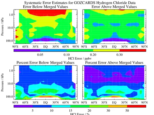
An indication of systematic errors in the merged values can be obtained by providing estimates of the range of available monthly mean source data. We have made such a calculation, although these error values are not part of the public GOZCARDS data files. For each bin, we computed the ranges of monthly means above and below the
20
merged values that include 95 % of the available source data monthly means. These er-ror bars are not usually symmetric about the merged values, especially if one dataset is biased significantly in relation to merged values. We did not have enough datasets here to consider a more statistical approach (such as actual SD among source datasets). Figure 5 shows the result of such a systematic error calculation at 46 hPa for the 35◦S
25
ACPD
15, 5849–5957, 2015Global OZone Chemistry And Related Datasets for
the Stratosphere (GOZCARDS)
L. Froidevaux et al.
Title Page
Abstract Introduction
Conclusions References
Tables Figures
◭ ◮
◭ ◮
Back Close
Full Screen / Esc
Printer-friendly Version
Interactive Discussion
Discussion
P
a
per
|
Discussion
P
a
per
|
Discussion
P
a
per
|
Discussion
P
a
per
|
averages at the 95 % boundaries have their own systematic errors (rarely smaller than 5 %), so our estimates do not really encompass all error sources. Error bars represent-ing a range within which 95 % of the source data values reside (see Figs. 5 and 6) can be a useful guide for data users or model comparisons; users can readily calculate such ranges (or we can provide these values).
5
Other quantities are provided in the netCDF GOZCARDS files, which are composed of one set of individual yearly files for all source datasets, and one set of yearly files for the merged products. The main data quantities are monthly averages, plus SD and standard errors for these means. The GOZCARDS source files also provide the number of days sampled each month as well as minimum and maximum values for
10
the source datasets. Other information includes average solar zenith angles and local solar times for individual sources. Note that for the species discussed here, sunset and sunrise occultation values in the same latitude bin during a given month are averaged together. Finally, formulae for monthly SD of the merged data are given in Appendix A, where sample time series of the SD and standard errors (not systematic errors) for
15
both source and merged HCl data are also shown.
3.3 GOZCARDS HCl sample results and discussion
Stratospheric HCl is important because it is the main reservoir of gaseous chlorine and it can be used to follow the chlorine budget evolution over the past decades. This includes a significant increase before the mid-1990s as a result of anthropogenic
chlo-20
rofluorocarbon (CFC) production, followed by a slower decrease as a result of the Mon-treal Protocol and subsequent international agreements to limit surface emissions that were correctly predicted to be harmful to the ozone layer (Molina and Rowland, 1974; Farman et al., 1985).
In Fig. 7, we provide an overview of the HCl evolution since 1991, based on
GOZ-25
ACPD
15, 5849–5957, 2015Global OZone Chemistry And Related Datasets for
the Stratosphere (GOZCARDS)
L. Froidevaux et al.
Title Page
Abstract Introduction
Conclusions References
Tables Figures
◭ ◮
◭ ◮
Back Close
Full Screen / Esc
Printer-friendly Version
Interactive Discussion
Discussion
P
a
per
|
Discussion
P
a
per
|
Discussion
P
a
per
|
Discussion
P
a
per
|
2000) and subsequent decreases. The GOZCARDS HCl time series for pressures less than 10 hPa stop in September 2010 because after this, v2.2 ACE-FTS data were halted, due to technical retrieval issues with that data version. Rates of decrease for stratospheric HCl and total chlorine have been documented based on such satellite-based upper stratospheric abundances, which tend to follow tropospheric source gas
5
trends with a time delay of order 6 years, with some uncertainties in the modeling of this time delay and related age of air issues (Waugh et al., 2001; Engel et al., 2002; Froidevaux et al., 2006). As summarized in WMO (2011), the average rate of decrease in stratospheric HCl has typically been measured at −0.6 to −0.9 % yr−1, in reason-able agreement with estimated rates of change in surface total chlorine; see also the
10
HCl upper stratospheric results provided by Anderson et al. (2000) for HALOE, Froide-vaux et al. (2006) for the one and a half year Aura MLS data record (from the initially used primary band), and Jones et al. (2009) and Brown et al. (2011) for a combi-nation of HALOE and ACE-FTS datasets. The WMO (2011) summary of trends also includes results from column HCl data at various NDACC Fourier transform infrared
15
(FTIR) measurement sites; see Kohlhepp et al. (2012) for a comprehensive discus-sion of ground-based results, showing some scatter as a function of latitude. Figure 7 demonstrates that a global-scale decline in mid- to lower stratospheric HCl is visible since about 1997. We also notice that at 68 hPa in the tropics, the long-term rate of change appears to be near-zero or slightly positive. In addition, there are shorter-term
20
periods in recent years when an average increasing “trend” would be inferred rather than a decrease, in particular, see the Northern Hemisphere data from 2005 through 2012 at 32 hPa.
To quantify the rates of change further, we created deseasonalized GOZCARDS merged monthly zonal mean HCl data for the different latitudes, and we show in Fig. 8
25
ACPD
15, 5849–5957, 2015Global OZone Chemistry And Related Datasets for
the Stratosphere (GOZCARDS)
L. Froidevaux et al.
Title Page
Abstract Introduction
Conclusions References
Tables Figures
◭ ◮
◭ ◮
Back Close
Full Screen / Esc
Printer-friendly Version
Interactive Discussion
Discussion
P
a
per
|
Discussion
P
a
per
|
Discussion
P
a
per
|
Discussion
P
a
per
|
stratosphere, depending on latitude. Some separation between northern and Southern Hemisphere results is observed in the lower stratosphere, with smaller trends in the Northern Hemisphere. Also, the scatter increases for 68 to 100 hPa and some positive (or essentially zero) trends occur at low latitudes in this region; however, we have less confidence in the results at 100 hPa, given the larger scatter and error bars in that
re-5
gion (and the smaller abundances). Results at more polar latitudes (not shown here) tend to follow the adjacent midlatitude bin results, but with more scatter (and larger error bars), especially for shorter time periods. To explore these rates of change in the lower stratosphere in more detail, Fig. 9 shows the same type of analysis as Fig. 8 for three other time periods and for pressures of 10 hPa or more: (Fig. 9a) for a decade of
10
data from 2003 through 2012, (Fig. 9b) for a shorter 6 year period from 2006 through 2011, and (Fig. 9c) for the most recent 6 year period from 2008 through 2013. For the results in (Fig. 9a), a decadal decrease is still observed for the Southern Hemisphere bins and some of the tropics in the upper region, but increases can be detected in the Northern Hemisphere and at the higher pressures in the tropics. In (Fig. 9b), we see
15
an accentuation of this hemispheric asymmetry in the short-term rates of change, with large positive changes in the Northern Hemisphere, and values on both negative and positive sides between 1 and 3 % yr−1 in many cases; during this past decade, this 6 year period (2006–2011) is near the temporal peak of this asymmetric lower strato-spheric behavior. In the most recent 6 year period, however (see Fig. 9c), the rates of
20
change have decreased for all the latitude bins shown, with all results from 10 to 68 hPa under 0.5 to 1 % yr−1 (absolute value). Without assigning an exact linear “trend” from these simple analyses, we illustrate here that there is considerable variability in lower stratospheric HCl short-term behavior, especially after 2005. Such lower stratospheric changes in HCl have been captured in column HCl FTIR data, as demonstrated by
25
ACPD
15, 5849–5957, 2015Global OZone Chemistry And Related Datasets for
the Stratosphere (GOZCARDS)
L. Froidevaux et al.
Title Page
Abstract Introduction
Conclusions References
Tables Figures
◭ ◮
◭ ◮
Back Close
Full Screen / Esc
Printer-friendly Version
Interactive Discussion
Discussion
P
a
per
|
Discussion
P
a
per
|
Discussion
P
a
per
|
Discussion
P
a
per
|
we note from Fig. 7, that such changes in lower stratospheric HCl appear to be fairly short-term in nature, with an apparent reversal in behavior occurring at both north-ern and southnorth-ern midlatitudes since 2011 (e.g., at 32 hPa). The lower stratospheric changes are distinct from the upper stratospheric long-term decrease, which we ex-pect to continue, as long as the Montreal Protocol agreements are fulfilled worldwide
5
and total surface chlorine emissions keep decreasing.
The rate of change analyses above were repeated and shown in Fig. 10 for slid-ing time periods centered on different years (e.g., a 6 year average for 2004 means an average from 2001 through 2006) in the upper and lower stratosphere for vari-ous latitude bins (covering 50◦S to 50◦N in 10◦ steps). As observed in Fig. 10a, the
10
sliding 6 year results indicate that there has been an acceleration in the rate of de-crease of upper stratospheric HCl between 2000 and 2004, followed by a flatter pe-riod until 2010 (this being the last year of GOZCARDS data available for the upper stratosphere, with a 6 year period centered at the start of 2008). The rate of upper stratospheric HCl change reached a maximum close to−1 % yr−1, and has retreated to
15
values near−0.5 % yr−1in more recent years. This is roughly in agreement with
time-shifted curves showing the rates of change for surface total chlorine based on National Oceanic and Atmospheric Administration (NOAA) surface data (Montzka et al., 1999), as shown in Fig. 10 (upper panels, green and purple curves) with the Earth System Research Laboratory Global Monitoring Division (website) data, time shifted by 6 or
20
7 years to approximately account for transport delays into the upper stratosphere. The tropospheric source gases for chlorine have also shown a reduction in the rate of de-crease during the 2nd half of the past decade, as discussed by Montzka et al. (1999) and summarized more recently in WMO (2011). As discussed in the latter report, this arises from a combination of factors, including the initial rapid decrease in methyl
chlo-25
ACPD
15, 5849–5957, 2015Global OZone Chemistry And Related Datasets for
the Stratosphere (GOZCARDS)
L. Froidevaux et al.
Title Page
Abstract Introduction
Conclusions References
Tables Figures
◭ ◮
◭ ◮
Back Close
Full Screen / Esc
Printer-friendly Version
Interactive Discussion
Discussion
P
a
per
|
Discussion
P
a
per
|
Discussion
P
a
per
|
Discussion
P
a
per
|
by considering the rates of change in partial column density between 68 and 10 hPa. The lower stratospheric rates of change show more variability with latitude than in the upper stratosphere for short (6 yr) time periods, and a hemispheric asymmetry exists, peaking in 2009, when positive tendencies are seen in the Northern Hemisphere, as opposed to decreases in the south. Figure 10c and d also displays the sensitivity to the
5
time period chosen, as we average the different latitudinal results (from the left panels) and add 8 year sliding periods to this analysis of HCl changes. The near-global results are not too dependent on whether 6 or 8 year periods are used, but longer periods tend to smooth out the rates of change; interannual changes, including those arising from the quasi-biennial oscillation (QBO), will affect short-term results, especially in the
10
lower stratosphere. It is worth noting (Fig. 10) that the patterns in the upper and lower stratosphere are qualitatively similar, and that rates of change in surface emissions will impact both regions, but carefully disentangling this from changes in the dynamics and in other constituents (e.g., CH4) that can affect the partitioning of chlorine species will require more analyses and modeling.
15
4 GOZCARDS H2O
4.1 GOZCARDS H2O source data records
We used water vapor datasets from HALOE, UARS MLS, ACE-FTS, and Aura MLS to generate the monthly zonal mean source products for GOZCARDS H2O.
In addition to the data screening procedures mentioned in Sect. 2, screening of
20
HALOE H2O data for high aerosol extinction values was performed, in a way very similar to the method used for the creation of merged H2O for the Stratospheric
Wa-ter vapor and OzOne Satellite Homogenized (SWOOSH) dataset (S. Davis, personal communication, 2012). This method (see Fig. S4) screens out anomalous HALOE H2O values that occurred mainly in 1991–1992, when the aerosol extinction near 22 hPa
ex-25
ACPD
15, 5849–5957, 2015Global OZone Chemistry And Related Datasets for
the Stratosphere (GOZCARDS)
L. Froidevaux et al.
Title Page
Abstract Introduction
Conclusions References
Tables Figures
◭ ◮
◭ ◮
Back Close
Full Screen / Esc
Printer-friendly Version
Interactive Discussion
Discussion
P
a
per
|
Discussion
P
a
per
|
Discussion
P
a
per
|
Discussion
P
a
per
|
corresponding H2O values. Also, for upper mesospheric HALOE data used here, care should be taken during high latitude summer months, as no screening was applied for the effect of polar mesospheric clouds (PMCs). High biases (by tens of percent) in H2O
above∼70 km have been shown to occur as a result of PMCs in the HALOE field of
view (McHugh et al., 2003). Indeed, monthly mean values larger than 8–10 ppmv are
5
observed in GOZCARDS H2O merged data and in HALOE source data for pressures
less than∼0.03 hPa. A more recent HALOE data version (version 20), or the version
labeled VPMC based on the above reference, could be used to largely correct such PMC-related effects, although this was not implemented for GOZCARDS H2O. The
Aura MLS and ACE-FTS measurements, obtained at longer wavelengths than those
10
from HALOE, do not yield such large H2O values; a rough threshold value of 8.5 ppmv could also be used (by GOZCARDS data users) to flag the pre-2005 merged dataset.
UARS MLS stratospheric H2O for GOZCARDS was obtained from V6 (or V600)
H2O data. This data version is identical to the original prototype (named V0104) from Pumphrey (1999), who noted that UARS MLS H2O often exhibits drier values (by 5– 15
10 %) than HALOE H2O (see also Pumphrey et al., 2000). The resulting GOZCARDS
H2O monthly zonal means span the period from September 1991 through April 1993. We note that a significant fraction of UARS MLS tropical data values at 100 hPa are flagged bad (as a result of diminishing sensitivity).
Summarizing briefly past validation results, SPARC WAVAS (2000) analyses pointed
20
out the existence of a small low bias in HALOE stratospheric data vs. most other measurements (from satellites or other means), except for UARS MLS. Lambert et al. (2007) showed agreement within 5–10 % between Aura MLS version 2.2 strato-spheric H2O and other satellite data, including ACE-FTS H2O (see also Carleer et al.,
2008), as well as for comparisons between Aura MLS and balloon data; Aura MLS
25
some-ACPD
15, 5849–5957, 2015Global OZone Chemistry And Related Datasets for
the Stratosphere (GOZCARDS)
L. Froidevaux et al.
Title Page
Abstract Introduction
Conclusions References
Tables Figures
◭ ◮
◭ ◮
Back Close
Full Screen / Esc
Printer-friendly Version
Interactive Discussion
Discussion
P
a
per
|
Discussion
P
a
per
|
Discussion
P
a
per
|
Discussion
P
a
per
|
what difficult to use as absolute validation of satellite-derived H2O in the upper tropo-sphere and lower stratotropo-sphere (UTLS) (Read et al., 2007; Weinstock et al., 2009). An intercomparison of measurements under controlled chamber conditions has helped to better constrain this issue (Fahey et al., 2014). Very good agreement exists between Aura MLS UTLS H2O and measurements from Cryogenic Frost point Hygrometers 5
(CFH), as discussed by Read et al. (2007) and Voemel et al. (2007) for MLS v2.2 data. At the lowest level (147 hPa) used here for merged H2O, the latter study showed a dry bias (by ∼10 %) in the MLS v2.2 data vs. CFH. Recent comparisons by Hurst et al. (2014) of MLS v3.3 H2O data vs. Boulder CFH time series show excellent overall
agreement, and no significant trend differences between coincident profile sets. There
10
is therefore support for systematic uncertainties as low as 5 % for lower stratospheric MLS data. Aura MLS stratospheric H2O v3.3 values are slightly larger (by up to∼5 %)
than the multi-instrument average from a number of satellite datasets, as discussed in SPARC Data Initiative comparisons by Hegglin et al. (2013). No large disagreements in interannual variations were noted by these authors for the GOZCARDS datasets
15
(p <150 hPa). From the mid-stratosphere to the upper mesosphere, excellent agree-ment between ground-based data from the Water Vapor Millimiter-wave Spectrometer (WVMS) and H2O profiles from Aura MLS and ACE-FTS has been demonstrated by
Nedoluha et al. (2007, 2009, 2011).
4.2 GOZCARDS H2O merged data records
20
The merging process for H2O is nearly identical to the method used for HCl. The main difference is an additional step that merges UARS MLS data with the already combined datasets from HALOE, ACE-FTS, and Aura MLS, by simply adjusting UARS MLS val-ues to the average of the previously merged series during the early (1991–1993) over-lap period; see Fig. S5 for an illustration at 22 hPa for the 5◦N latitude bin. Typically, this
25
requires an upward adjustment of the UARS MLS H2O data, as these values are biased
ACPD
15, 5849–5957, 2015Global OZone Chemistry And Related Datasets for
the Stratosphere (GOZCARDS)
L. Froidevaux et al.
Title Page
Abstract Introduction
Conclusions References
Tables Figures
◭ ◮
◭ ◮
Back Close
Full Screen / Esc
Printer-friendly Version
Interactive Discussion
Discussion
P
a
per
|
Discussion
P
a
per
|
Discussion
P
a
per
|
Discussion
P
a
per
|
H2O (and following past advice from the SAGE II team itself), we decided to use caution and did not include that dataset for GOZCARDS merging, as some trend results could be affected to an unknown extent. Also, there is probably some remaining retrieval con-tamination from volcanic aerosol effects for some time after the volcanic eruptions of El Chichon (1982) and Mt. Pinatubo (1991), as well as after several smaller eruptions;
5
see Bauman et al. (2003) for a review of stratospheric aerosol climatology (1984–1999) and Thomason et al. (2008) for the SAGE II stratospheric aerosol dataset.
Minor procedural merging details or issues for H2O are included in the Supplement.
Also, data users should be aware of effects from unequal latitudinal sampling when no MLS data exist, for regions where large latitudinal variations occur, as for H2O at
10
147 hPa (the largest pressure value). Indeed, global or latitudinal averages can be sig-nificantly biased in certain months and month-to-month variability for such averages increases. This is because of poor sampling of the full latitudinal variability, prior to Au-gust 2004; after this, regular sampling exists from MLS every month. Such variations in sampling can become an issue for temporal analyses of latitudinal or global averages,
15
unless additional fits or interpolations to mitigate such effects are undertaken.
In Fig. 11, we display the average offsets that were applied to the four H2O source datasets; these offsets follow previously known relative data biases (mentioned ear-lier). For example, low biases in UARS MLS H2O, especially in the mesosphere, were
discussed by Pumphrey (1999) and the UARS MLS offsets (see Fig. 11) correct that
20
dataset upward. The application of offsets derived for HALOE and UARS MLS raises the H2O time series from these instruments, whereas negative offsets lower the H2O
source data from ACE-FTS and Aura MLS. As we found for HCl, the offset values generally display small variations vs. latitude and are therefore fairly stable systematic adjustments to the time series. Figure S6 displays the amplitudes of the fitted annual
25
ACPD
15, 5849–5957, 2015Global OZone Chemistry And Related Datasets for
the Stratosphere (GOZCARDS)
L. Froidevaux et al.
Title Page
Abstract Introduction
Conclusions References
Tables Figures
◭ ◮
◭ ◮
Back Close
Full Screen / Esc
Printer-friendly Version
Interactive Discussion
Discussion
P
a
per
|
Discussion
P
a
per
|
Discussion
P
a
per
|
Discussion
P
a
per
|
Aura MLS high southern latitude data. Figure 12 provides some statistical information, as done for HCl in Sect. 3.2, regarding the correlations and trend differences between ACE-FTS and Aura MLS. There are a few regions with noisier relationships. While slow increases in H2O are generally observed by both instruments in the stratosphere and mesosphere, the tropical region near 0.1 hPa shows a slight decreasing trend for the
5
ACE-FTS points, thus leading to larger discrepancies; it is not clear what the source of these discrepancies is. While the tropical ACE-FTS data are generally sampled with a significantly lower temporal frequency, the same applies for all pressure levels; how-ever, a few outlier points can have a much larger impact when sampling is poorer. There are also a few other spots, such as near 65◦S and 65◦N and near 5 hPa with a poor
10
trend value for the difference series, in comparison to the errors; this may be caused by a combination of poorer sampling by ACE-FTS and higher atmospheric variability, which can lead to more scatter. At the highest latitudes in the lower stratosphere, the observed slope differences are more within error bars, but the larger variability means that a longer record is needed to determine if two time series really trend differently.
15
The main point here is to show the dataset characteristics and to point out where the agreement is better or worse than typical. The merged dataset tends to be much closer to Aura MLS in terms of trends because there are usually many more months of Aura MLS data than ACE-FTS data, including the fact that the ACE-FTS time series (data version 2.2) used here was halted for data after late 2010 due to technical retrieval
20
issues. Therefore, the overall impact of ACE-FTS data on the merged H2O series is
fairly small.
Figure S7 provides a visual representation of the merged GOZCARDS H2O fields at 3 and 68 hPa, respectively. Well-known features are displayed in these plots, given the good global coverage in the post-2004 period in particular. In the upper stratosphere,
25
tem-ACPD
15, 5849–5957, 2015Global OZone Chemistry And Related Datasets for
the Stratosphere (GOZCARDS)
L. Froidevaux et al.
Title Page
Abstract Introduction
Conclusions References
Tables Figures
◭ ◮
◭ ◮
Back Close
Full Screen / Esc
Printer-friendly Version
Interactive Discussion
Discussion
P
a
per
|
Discussion
P
a
per
|
Discussion
P
a
per
|
Discussion
P
a
per
|
peratures and has been measured in satellite data since the early 1990s (Mote et al., 1996; Pumphrey, 1999). A vertical cross-section of this lower stratospheric tropical (20◦S to 20◦N) tape recorder in GOZCARDS merged H2O for 1991–2013 is shown
in Fig. 13; periods of positive anomalies alternate with negative anomalies, including the post-2000 lows, as well as the most recent decreases in 2012–2013 (see also next
5
section).
As we discussed for HCl, we have estimated systematic errors for the merged H2O product. This is illustrated by the contour plots in Fig. 14; these ranges encompass at least 95 % of the monthly mean source data values from HALOE, UARS MLS, ACE-FTS, and Aura MLS above or below the merged series. These errors typically span 5 to
10
15 % of the mean between 100 and 0.1 hPa; errors larger than 30 % exist in the tropical upper troposphere (147 hPa), and similarly, large values in the upper mesosphere arise from the low bias in UARS MLS H2O.
4.3 GOZCARDS H2O sample results and discussion
Stratospheric H2O variations have garnered attention in the past two decades, be-15
cause of the radiative impacts of water vapor in the UTLS and the connection to climate change, as well as the stratospheric chemical significance of H2O oxidation products. H2O can influence changes in stratospheric and mesospheric ozone via the HOx cat-alytic cycles. H2O in the UTLS has a significant radiative impact (e.g., Forster and
Shine, 2002) and has the potential to influence surface temperature changes in ways
20
that could mitigate surface warming (Solomon et al., 2010) if H2O exhibits a signifi-cant drop, as was observed right after 2000. A decrease of about 1 ppmv was also observed in in situ data (Fujiwara et al., 2010; Hurst et al., 2011; Kunz et al., 2013). Randel et al. (2004, 2006) correlated this post-2000 decrease with a decline in tropi-cal cold point temperatures. An increasing trend in stratospheric H2O since the 1950s 25
ACPD
15, 5849–5957, 2015Global OZone Chemistry And Related Datasets for
the Stratosphere (GOZCARDS)
L. Froidevaux et al.
Title Page
Abstract Introduction
Conclusions References
Tables Figures
◭ ◮
◭ ◮
Back Close
Full Screen / Esc
Printer-friendly Version
Interactive Discussion
Discussion
P
a
per
|
Discussion
P
a
per
|
Discussion
P
a
per
|
Discussion
P
a
per
|
Reid, 2008; Garfinkel et al., 2013). Efforts to better understand past changes in H2O, and their causes and expected impacts, include the references above, and (among others) Dvortsov and Solomon (2001), Shindell (2001), Nedoluha et al. (2003), Ur-ban et al. (2007), Dhomse et al. (2008), Scherer et al. (2008), Read et al. (2008), Tian et al. (2009), Schoeberl et al. (2012), Fueglistaler (2012), Fueglistaler et al. (2013), and
5
the recent review of the tropical tropopause layer by Randel and Jensen (2013). The reconciliation of long-term trends in tropopause temperatures with changes in lower stratospheric water vapor is a task worthy of continued study, using additional datasets as well as model studies.
Individual water vapor datasets have been used here to produce a merged record
10
now spanning more than two decades. Linear trend estimates can be quite sensitive to the starting and ending points of the time series, even for 22 years of data, and simple linear trends do not best describe the variations in stratospheric H2O over the past two
decades. We do not attempt here to characterize trends or to imply that recent ten-dencies will carry into the next decade or two. Rather, as variability is also of interest
15
to climate modelers, we provide information below regarding observed decadal-type (longer-term) variability in stratospheric water vapor. Figure 15 illustrates monthly, an-nual, and longer-term changes in stratospheric water vapor, based on the global GOZ-CARDS merged H2O series; this shows the well-known H2O minimum in the lower
tropical stratosphere as well as an increasing vertical gradient in the upper
strato-20
sphere (as a result of methane oxidation). As we know from past studies (e.g., Randel et al., 2004), medium- to long-term changes in H2O are large-scale in nature. However,
lower stratospheric H2O variations are more accentuated at low latitudes, in compari-son to near-global (60◦S–60◦N) results. It has long been known (e.g., from the in situ balloon-borne measurements of Kley et al., 1979) that the hygropause is typically
lo-25
ACPD
15, 5849–5957, 2015Global OZone Chemistry And Related Datasets for
the Stratosphere (GOZCARDS)
L. Froidevaux et al.
Title Page
Abstract Introduction
Conclusions References
Tables Figures
◭ ◮
◭ ◮
Back Close
Full Screen / Esc
Printer-friendly Version
Interactive Discussion
Discussion
P
a
per
|
Discussion
P
a
per
|
Discussion
P
a
per
|
Discussion
P
a
per
|
the tropics (20◦S–20◦N) have varied between about 3.2 and 4.2 ppmv at 68 hPa. The rapid drop between 2000 and 2001 is observed at 100 and 68 hPa, with some dilu-tion of this effect at higher altitudes. There is a clear difference in long-term behavior between the upper stratosphere, where changes in methane should have the clearest influence, and the lower stratosphere, especially in a narrow vertical region above the
5
tropopause, where cold point temperatures and dynamical changes have a significant impact. To first-order, the last few years show∼10 % larger values in the upper
strato-sphere than in the early 1990s, while the opposite holds in the lowest stratospheric re-gion, where a decrease of order 10 % is observed over the same period. The long-term upper stratospheric increase carries into the mesosphere (see below). Figure 15 also
10
shows that month-to-month and seasonal variations (thin lines) are usually somewhat larger than the long-term changes in the lower stratosphere, most notably at 100 hPa.
In order to provide longer-term variability diagnostics for water vapor, we show in Fig. 16 the minimum to maximum spread in annual averages (tropics and mid-latitudes) from Fig. 15. These variability diagnostics are provided for the 22 year period (1992
15
to 2013) and also separated into the two 11 year periods (thin and dashed lines); as expected, the 22 year variability is always larger than the variability in either of the two decadal period subsets. We also note that the tropical variability is largest just above the tropopause (here this means at the 68 hPa GOZCARDS level), where it reaches 20–28 % (or 0.8 to 1 ppmv) depending on the time period. Such variability diagnostics
20
should be useful for comparisons to various chemistry climate models.
The longer-term variability in water vapor increases above the stratopause and reaches close to 30 % in the uppermost mesosphere, as seen in Fig. 17a; this plot shows the monthly and annual near-global (60◦S–60◦N) H2O variations at 0.01 hPa.
Large seasonal changes in this region are driven by vertical advection associated with
25