www.atmos-chem-phys.net/11/1227/2011/ doi:10.5194/acp-11-1227-2011
© Author(s) 2011. CC Attribution 3.0 License.
Chemistry
and Physics
Results from a new linear O
3
scheme with embedded heterogeneous
chemistry compared with the parent full-chemistry 3-D CTM
B. M. Monge-Sanz1, M. P. Chipperfield1, D. Cariolle2,3, and W. Feng1
1Institute for Climate and Atmospheric Science, School of Earth and Environment, University of Leeds, Leeds, UK 2Centre Europ´een de Recherche et Formation Avanc´ee en Calcul Scientifique, Toulouse, France
3M´et´eo-France, Toulouse, France
Received: 23 April 2010 – Published in Atmos. Chem. Phys. Discuss.: 20 May 2010 Revised: 21 January 2011 – Accepted: 26 January 2011 – Published: 14 February 2011
Abstract.A detailed full-chemistry 3-D chemistry and trans-port model (CTM) is used to evaluate the current strato-spheric O3 parameterisation in the European Centre for Medium-Range Weather Forecasts (ECMWF) model and to obtain an alternative version of the ozone scheme implicitly including heterogeneous chemistry. The approach avoids the inaccurate treatment currently given to heterogeneous ozone chemistry in the ECMWF model, as well as the uncertainties of a cold-tracer. The new O3 scheme (COPCAT) is eval-uated within the same CTM used to calculate it. It is the first time such a comparison has been possible, providing di-rect information on the validity of the linear parameterisa-tion approach for stratospheric ozone. Simulated total col-umn and O3profiles are compared against Total Ozone Map-ping Spectrometer (TOMS) and Halogen Occultation Exper-iment (HALOE) observations. COPCAT successfully simu-lates polar loss and reproduces a realistic Antarctic O3hole. The new scheme is comparable to the full-chemistry in many regions for multiannual runs. The parameterisation produces less ozone over the tropics around 10 hPa, compared to full-chemistry and observations. However, this problem can be ameliorated by choosing a different ozone climatology for the scheme. The new scheme is compared to the current ECMWF scheme in the same CTM runs. The Antarctic O3 hole with the current ECMWF scheme is weaker and disap-pears earlier than with the new COPCAT scheme. Differ-ences between the current ECMWF scheme and COPCAT are difficult to explain due to the different approach used for heterogeneous chemistry and differences in the photochem-ical models used to calculate the scheme coefficients. Re-sults with the new COPCAT scheme presented here show
Correspondence to:B. M. Monge-Sanz ([email protected])
that heterogeneous and homogeneous ozone chemistry can be included in a consistent way in a linear ozone parameteri-sation, without any additional tunable parameters, providing a parameterisation scheme in better agreement with the cur-rent knowledge of stratospheric O3chemistry than previous approaches.
1 Introduction
and loss (L), where the net production (P−L) is consid-ered a linear function of ozone mixing ratio (f), tempera-ture (T) and partial column of ozone above the point con-sidered (cO3). The coefficients for the linearisation are ob-tained from a photochemical model and provided as look-up tables which are functions of latitude, level and month of the year. The photochemical models used until now to derive the coefficients have included only gas-phase chemistry (Cari-olle and D´equ´e, 1986; Cari(Cari-olle and Teyss`edre, 2007; McCor-mack et al., 2006) or very limited heterogeneous processes (McLinden et al., 2000), which has made it necessary to in-clude an additional term in the parameterisation to take into account heterogeneous chemistry.
The European Centre for Medium-Range Weather Fore-casts (ECMWF) model uses a linear parameterisation for O3 based on the CD approach. The O3 coefficients for the CD scheme used by the ECMWF model (Dethof and H´olm, 2004) are derived from the 2-D photochemical model MOBIDIC (Cariolle and Teyss`edre, 2007). The complete ECMWF scheme is based on the expression
∂f
∂t =c0+c1(f− ¯f )+c2(T− ¯T )+c3(cO3− ¯cO3)+c4(ClEQ)
2f (1)
wheref¯,T¯ andc¯
O3 are climatological reference values for local O3, temperature and partial column of O3. The coeffi-cientsci(i=0, 1, 2, 3, 4) are derived from the photochemical model. The fifth term on the right hand side of Eq. (1) corre-sponds to the additional heterogeneous term used in the cur-rent ECMWF parameterisation. ClEQis the equivalent chlo-rine content of the stratosphere, and is the only parameter that varies from year to year. This fifth term is only active when temperature falls below 195 K in daytime for latitudes pole-ward of 45◦. This ECMWF ozone scheme version (currently operational) is also denoted here v2.9 after the version of co-efficients provided by M´et´eo France. Other versions follow-ing the same conceptual CD approach are LINOZ (McLinden et al., 2000) and CHEM2D (McCormack et al., 2004, 2006). Geer et al. (2007) gives a comparison of several versions of ECMWF, LINOZ and CHEM2D coefficients in terms of their performance in a data assimilation system. However, none of these schemes includes a complete heterogeneous descrip-tion, and all of them need an extra term for the simulation of O3polar loss. In Geer et al. (2007) heterogeneous processes were parameterised by means of a cold tracer (Eskes et al., 2003) for all the evaluated O3schemes.
The CD scheme first appeared in the 1980s, when knowl-edge of the importance of heterogeneous O3chemistry was very limited. Therefore, in its original version the CD pa-rameterisation lacked a heterogeneous term. More recent versions (Cariolle and Teyss`edre, 2007) were computed in a similar way to their predecessor: omitting heterogeneous chemistry but including an additional term calculated with different methods and approximations and, thus, not consis-tent with the gas-phase chemistry described by the scheme. This separation between gas-phase and heterogeneous
reac-tions reduces the accuracy of the ECMWF approach. The use of a localised heterogeneous term (i.e. the 5th term in Eq. 1) produces too weak polar ozone loss in the ECMWF global model, unless O3 observations are assimilated (De-thof and H´olm, 2004). Conceptually, this kind of term is too restrictive with respect to the current understanding of heterogeneous processes. First, the temperature threshold for the formation of polar stratospheric clouds (PSCs) ac-tually depends on altitude and trace gas concentrations. The adopted sharp threshold temperature of 195 K in Eq. (1) is representative of an altitude of ∼20 km and 5 ppbv HNO3 (e.g. Hanson and Mauersberger, 1988; Carslaw et al., 1994). For a more realistic scheme, the temperature threshold in the heterogeneous term should include altitude dependency, and whenever possible be linked to the concentrations of H2O, HNO3and H2SO4aerosol. Second, for the long-term evolu-tion of polar ozone loss, the actual heterogeneous chemistry loss is not proportional to the square of the chlorine content (Cl2EQ). As shown by Searle et al. (1998), an exponent value of 1.5 is much more representative of the typical conditions encountered in a fully activated polar vortex. In addition, not only do chlorine cycles play a role in destroying polar ozone, the ClO+BrO cycle can account for up to 50% of the polar depletion, and for this latter cycle the Cl dependency is linear. So, by considering the ozone loss to be quadratic in Cl2EQ, the ECMWF scheme would not capture the correct decadal trend. The amount of O3 destruction simulated by ECMWF for present conditions is insufficient (Dethof and H´olm, 2004), and the Antarctic hole tends to last shorter than observed. This means that if the scheme is used for earlier years the quadratic dependence on Cl will decrease making the ozone loss even smaller compared to observations.
Another fundamental shortcoming of the heterogeneous approach in Eq. (1) is that it assumes chlorine activation and O3 destruction by sunlight to take place at the same time. In reality, the activation of air masses takes place during the polar night inside the polar vortex, when temperature is low enough. Later, with the return of spring sunlight to polar lat-itudes, the processed air is able to destroy ozone. However, the destruction can also happen during winter if activated air masses can reach lower latitudes (e.g. by filamentation or vortex break-up) and be exposed to sunlight. This latter kind of process is completely missed by a localised temperature term like the one in the ECMWF scheme (Eq. 1).
to the current ECMWF heterogeneous term (Cariolle and Teyss`edre, 2007), however, a cold-tracer also has intrinsic problems due to the number of tunable parameters it requires (e.g. activation/deactivation times and destruction rate). This makes this kind of tracer somewhat arbitrary and difficult to adapt to the atmospheric variability found in, for instance, a reanalysis time series; as meteorological and chemical con-ditions change, the same cold-tracer parameters would not be equally valid for every year. Additionally, the cold-tracer ap-proach, by definition, requires an extra tracer to keep track of the low temperature air masses, which adds undesired com-putational cost to the NWP simulations.
To avoid the artificial split between gas-phase and hetero-geneous processes, a better conceptual approach can be ex-plored, which represents a good compromise between the re-alistic heterogeneous full-chemistry and a simple one-tracer parameterisation. Such approach is the use of a scheme of the form described in Eq. (1) but, instead of using the addi-tional 5th term, using an alternative set of coefficients (c0,
c1,c2 andc3) that implicitly includes heterogeneous ozone chemistry.
This new approach is proposed and evaluated in the present study. Here, based on the CD linear approach, a new set of coefficients is obtained from the 3-D chemistry transport model (CTM) TOMCAT/SLIMCAT (Chipperfield, 2006) including complete heterogeneous processes. The al-ternative ozone scheme COPCAT (Coefficients for Ozone Parameterisation from a Chemistry And Transport model) does not need any additional heterogeneous term as it im-plicitly includes heterogeneous chemistry in the first 4 co-efficients (Monge-Sanz, 2008). In the new scheme long-term changes in stratospheric chlorine (or odd nitrogen, wa-ter vapour etc.) can be taken into account in a consistent way by deriving coefficients from the CTM for different periods. This new COPCAT approach is a more natural way to include both gas-phase and heterogeneous processes, and is expected to improve not only the representation of polar ozone, but has also the advantage of including mid-latitude heterogeneous processes that have been so far ignored by most O3 linear schemes.
In addition, from existing literature it is difficult (if not impossible) to discern whether the limitations of the linear ozone schemes come from the parameterisation approach, from the photochemical model used to obtain the coeffi-cients, or even from the 3-D model where the scheme is implemented. Obtaining a new scheme based on TOM-CAT/SLIMCAT, a widely used and evaluated 3-D CTM, helps to clarify which problems are due to the parameteri-sation approach as distinct from the limitations of the parent photochemical model. This study presents the first compari-son between a linear ozone parameterisation and the equiva-lent full chemistry 3-D model used to calculate it.
In this paper, Sect. 2 describes the calculation of the new COPCAT scheme. The observations used to validate model results are briefly described in Sect. 3. The parameterisation
performance is shown in Sect. 4, where the new scheme is compared with SLIMCAT full-chemistry runs and the cur-rent ECMWF scheme within CTM runs. This section also includes further polar results showing the ability of COPCAT to adapt to different meteorological conditions. A final sum-mary of results and future work and applications is given in Sect. 5.
2 COPCAT scheme
2.1 Coefficients calculation
To calculate the parameterisation coefficients, the TOM-CAT/SLIMCAT box model was used. The box model config-uration is identical to the 3-D CTM (chemical descriptions, resolution etc.) but it does not consider transport processes. The box model was initialised from the 3-D model output and a series of short sensitivity runs were performed as described here below. The box model short runs were initialised with the zonally averaged output of the full-chemistry 3-D model run 323. Run 323 is a multiannual SLIMCAT run that uses a 7.5◦×7.5◦horizontal resolution and 24 vertical levels (L24).
The run 323 is driven by ERA-40 winds (Uppala et al., 2005) from 1977–2001 and by ECMWF operational winds from 2002–2006. The SLIMCAT fields used to initialise the box model correspond to January–December 2000. SLIMCAT data for the 15th of each month are passed to the box model as initialisation, then, from that initial state, seven 2-day runs of the box model were carried out; one control run and six perturbation runs from the initial conditions. The resolu-tion adopted for the box model is 24 latitudes, and 24 lev-els (from the surface up to∼60 km), matching the resolution of the full-chemistry run used for the initialisation. The box model also uses the same chemistry module as the full SLIM-CAT model. The short runs of the CTM in box model mode were used to compute the ozone tendencies in the COPCAT scheme (Monge-Sanz, 2008). In these runs the chemistry was computed every 20 min.
a)
(P-L)0 SEPCOPCAT
b)
(P-L)0 SEPCariolle v2.9
c)
(P-L)0 SEPLINOZ
d)
(P-L)0 SEPCHEM2D
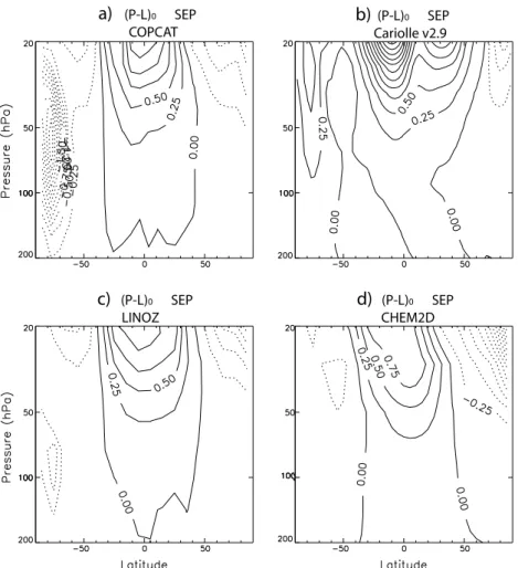
Fig. 1.Altitude/latitude distribution ofc0(see text in Sect. 1 for details), in ppmv/month, for the month of September for(a)COPCAT,(b) ECMWF v2.9(c)LINOZ and(d)CHEM2D. Contour intervals are 0.25 ppmv/month.
based on the daily net production of O3 averaged over the last day of the run (second day in this case). For the ozone perturbed runs (local ozone and column), O3on the second day of the run is initialised with the average field over the first day. The whole calculation procedure is applied to every month of the year. This methodology provides 7 coefficients for each month, on 24 latitudes and 24 vertical levels. The 12 files corresponding the monthly coefficients can then be read in by a CTM or a general circulation model (GCM) simula-tion in which ozone (f) is treated as a tracer following the COPCAT approach
∂f
∂t =c0+c1(f− ¯f )+c2(T− ¯T )+c3(cO3− ¯cO3). (2)
2.2 Implicit heterogeneous chemistry
A 3-D model using COPCAT coefficients can successfully simulate polar and mid-latitude O3depletion despite the fact that no additional heterogeneous term is included. By plot-ting the September reference net production(P−L)0, i.e.c0, in the lower stratosphere (LS) for the different schemes
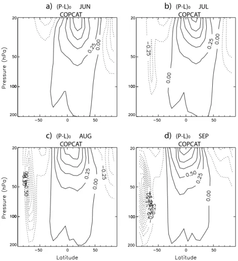
(Fig. 1), it can be seen that COPCAT shows a depletion region centred at 50 hPa over the south pole. This repre-sents the ozone destruction caused by PSCs triggered by spring sunlight. None of the other schemes shows such a depletion region; only LINOZ shows a weak loss region at 100 hPa over southern high latitudes, but it is not enough to produce spring ozone depletion over the Antarctic. Fig-ure 2 shows the evolution of COPCATc0coefficient in June– September in the LS. The Antarctic loss region starts to de-velop at the edge of the vortex in July; in September values of −2.1 ppmv/month are reached around 40 hPa at high south-ern latitudes.
2.3 Linearity validation
a)
(P-L)0 JUN COPCATb)
(P-L)0 JUL COPCATc)
(P-L)0 AUG COPCATd)
(P-L)0 SEP COPCATFig. 2.Altitude/latitude distribution of COPCAT net ozone productionc0(see text in Sect. 1 for details), in ppmv/month, for(a)June,(b) July,(c)August and(d)September. Contour intervals are 0.25 ppmv/month.
were found to be less than 1% for variations of±20% in the value off. For LINOZ, McLinden et al. (2000) showed the deviations from the linear tendencies in (P−L) with respect tof,cO3 andT, which were low enough to consider the lin-ear approximation valid for the usual range of variability ob-served in GCMs. Also, McCormack et al. (2006) showed the linearity in CHEM2D was valid for variations of±20 K in temperature and±50% in ozone column. Analysing the lin-ear approximation in the COPCAT scheme is also necessary, since the previous schemes did not include any polar het-erogeneous chemistry implicitly, and only LINOZ included processes on binary sulfate aerosols.
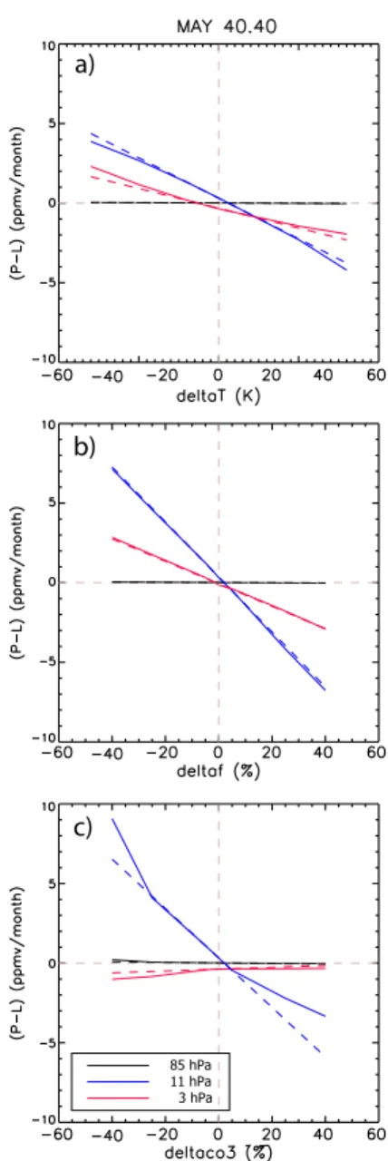
Figure 3 shows the COPCAT (P−L) values as a func-tion of perturbafunc-tion of local ozonef, temperatureT and col-umn abovecO3 for three vertical levels, at 40◦N in May. The ranges of variation, with respect to the reference state, chosen for the three variables are±40% in local ozone and column and±16 K in temperature. The vertical levels represented correspond to 85 hPa, 11 hPa and 3 hPa. The exact tendency has been represented together with the linear squares fit to the points obtained using the same perturbation values, three for
each variable, employed to obtain the COPCAT coefficients. A standard least-squares fit method was chosen, so that the linear fit is easy to generalise to a larger number of points and also comparable to linear validations performed for pre-vious CD-like ozone schemes (e.g. McCormack et al., 2006). Results in Fig. 3 show that the linearisation is a good approx-imation for the three variables in the ranges shown and only the dependence oncO3 shows some non-linearity for column variations larger than±20%.
The level of agreement with the linear approximation shown in Fig. 3 is similar for other months and latitudes, ex-cept for polar LS regions in spring. Figure 4 evaluates the linear approximation in the LS at 84◦S in September. The
85 hPa 11 hPa 3 hPa
a)
c) b)
Fig. 3. COPCAT (P-L) values as a function of the perturbation in (a)temperatureT,(b)local ozonef and(c)column abovecO3, at 40◦N in May. Pressure levels shown are 85 hPa (black), 11 hPa (blue) and 3 hPa (red). Solid lines correspond to the exact ten-dencies from the box model; dashed lines correspond to the least squares fit for the perturbation values used for COPCAT coefficients (Sect. 2). To show all results within the same vertical axis, those for the 3 hPa level have been scaled by 0.1, 0.25 and 0.1 forT,f and
cO3respectively.
activation due to denitrification is not a sharp step but more of a smooth threshold. Chlorine activation on cold sulfate aerosol near the PSC formation threshold causes activation rates to vary in this way.
These results show that the linear approximation is also a good estimation for the O3 scheme developed here. De-spite including heterogeneous chemistry implicitly COPCAT agrees with a linear approximation for local ozone variations
85 hPa 111 hPa 52 hPa
a)
c) b)
Fig. 4.Same as Fig. 3 but for the polar lower stratosphere at 84◦S in September. Represented pressure levels are 111 hPa (black), 85 hPa (blue) and 52 hPa (red).
3 Ozone observations
We compare model results in this work against Total Ozone Mapping Spectrometer (TOMS) column observations (McPeters et al., 1998), and O3 data from the Halogen Oc-cultation Experiment (HALOE) (Br¨uhl et al., 1996).
3.1 TOMS data
TOMS provided a near-continuous record of ozone measure-ments from 1978 to December 2005, with a high-density horizontal coverage of total ozone of about 200 000 ob-servations per day (only daylight measurements). TOMS data have been widely used for the validation of models and other observational sets. Monthly data of TOMS Earth Probe (EP) (McPeters et al., 1998) have been obtained from http://toms.gsfc.nasa.gov/. Zonal monthly means are avail-able from 85◦N–85◦S with a 5◦resolution. McPeters et al.
(1998) includes a detailed description of errors for EP/TOMS total ozone. They estimated the absolute error to be of 3% and the random error of 2%; larger errors (up to 6%) may ex-ist due to the presence of Type II PSCs at solar zenith angles greater than 80 degrees.
3.2 HALOE O3data
Br¨uhl et al. (1996) provided the most comprehensive val-idation study for HALOE ozone data. Since that valida-tion study, HALOE has gone through two major revisions. The HALOE data used in our study correspond to the third public release v19 (William Randel and Fei Wu, personal communication). Comparison of these HALOE ozone data with Stratospheric Aerosol and Gas Experiment (SAGE) II measurements was carried out in Morris et al. (2002) and McHugh et al. (2005) compared them against Atmospheric Chemistry Experiment (ACE) observations. We have used HALOE O3monthly data zonally averaged, available for 41 latitudes (80◦N–80◦S) and 49 pressure levels (from 100–
0.01 hPa). HALOE O3data agree to within 10% of their co-incident ozonesonde measurements down to 100 hPa at trop-ical/subtropical latitudes and to 200 hPa at extratropical lati-tudes (e.g. Bhatt et al., 1999). HALOE data have very high vertical resolution (2 km), however, there are few observa-tions for some individual months, so HALOE annual aver-aged values have been used here only when comparing with annually averaged results from the model runs. HALOE O3 data (Br¨uhl et al., 1996) have been used for evaluating numer-ous models (e.g. Chipperfield et al., 2002; Steil et al., 2003; Eyring et al., 2006; Feng et al., 2007).
4 Performance of the COPCAT scheme
The way COPCAT coefficients have been calculated enables for the first time the comparison between the parameterisa-tion and the full-chemistry CTM used to obtain it. In this
a)
b) d)
c)
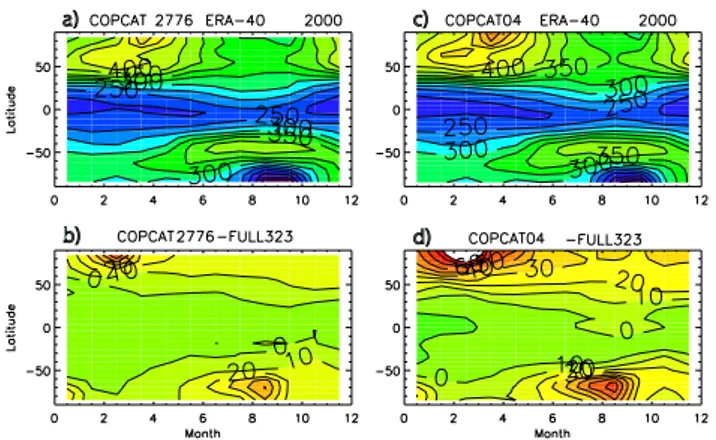
Fig. 5. Total ozone column (DU) from(a)COPCAT scheme,(b) differences COPCAT-SLIMCAT full-chemistry. The equivalent run using COPCAT04 (coefficients based on year 2004 meteorology) is shown in(c)and the corresponding differences with full-chemistry in(d). All simulations use ERA-40 winds for year 2000. Contour interval for (a) and (c) is 25 DU and 10 DU for differences in(b) and(d). For panels(a)and(c)the colour scale goes from dark blue (lowest ozone) to red (highest ozone). For(b)and(d)colours range from dark green (most negative difference) to red (most positive difference).
way, the same numerics and dynamics are involved and dif-ferences can only be due to the use of the COPCAT scheme instead of the full-chemistry. This kind of evaluation was not possible for previous linear O3parameterisations, since they were computed by 2-D photochemical models and then implemented within 3-D GCMs or CTMs.
4.1 Comparison with full-chemistry simulations
The SLIMCAT full-chemistry run 323 (Sect. 2) is in good general agreement with TOMS (Monge-Sanz, 2008) and the temporal and spatial evolution of O3 is well simulated. In particular, the minimum in the Southern Hemisphere spring is accurately represented by SLIMCAT in multiannual runs (e.g. Chipperfield, 1999, 2003).
4.1.1 Total ozone column
84ºN
84ºS
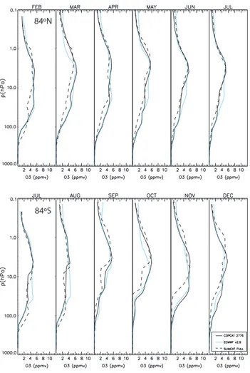
Fig. 6. Zonally averaged ozone profiles (ppmv) on the 15th of February–July 2000 at 84◦N (top), and July–December at 84◦S (bottom), from COPCAT tracer (solid black line), ECMWF v2.9 (dotted blue line) and SLIMCAT full-chemistry (dashed black line).
40 DU higher than the full-chemistry. The situation over the Arctic is very similar, differences are below 20 DU except in winter/spring. However, maximum differences over the Arc-tic are larger than in the AntarcArc-tic, reaching up to 60 DU in March.
4.1.2 Sensitivity to the meteorological conditions in the coefficients calculation
The default version of COPCAT used and described in this study has been derived under meteorological conditions for the year 2000 (Sect. 2.1). The reason for this was to en-sure that the scheme is able to reproduce the ozone tenden-cies found in a cold winter. As 2000 was particularly cold over the Arctic (e.g. Sinnhuber et al., 2000), the scheme will then be able to generalise to both cold and milder conditions. To show the sensitivity the COPCAT coefficients present to the meteorology used for its calculation we have also derived a version of the scheme based on meteorology for the year
2004 (COPCAT04), a year which showed relatively mild temperatures during the Arctic winter (e.g. Manney et al., 2005).
Figure 5c shows the January–December 2000 total ozone (TO) column simulated by COPCAT04 and Fig. 5d the dif-ferences with respect to the full-chemistry run 323. The cor-responding CTM runs were completely equivalent to those used to obtain the results shown in Figs. 5a and b, i.e. the CTM was driven by ERA-40 for year 2000 and the only dif-ference is in the version of the coefficients used in the runs. It can be seen how the COPCAT04 coefficients produce sig-nificantly higher concentrations over the poles, compared to the default COPCAT ones. Over the Arctic winter/spring column values with COPCAT04 are over 30 DU larger than with COPCAT, while over the Antarctic spring COPCAT04 is around 20 DU higher than the default COPCAT. These re-sults indicate that basing the coefficients on a year with mild temperatures (e.g. 2004) restricts the ability of the scheme to reproduce realistic ozone loss during colder winters (e.g. year 2000). On the other hand, basing the coefficients on a cold year allows the scheme to adapt also to milder condi-tions, as will be shown later in Sect. 4.3. Most of the results shown hereafter correspond to the COPCAT default version based on meteorology for the year 2000, otherwise the nota-tion COPCAT04 will be clearly specified.
4.1.3 Ozone vertical profiles
Total ozone column is a good diagnostic for the global vari-ability achieved by the model both in time and space. How-ever, the vertical distribution of O3 must also be realistic in order to simulate correct radiative fluxes at all levels in the atmosphere. Figure 6 shows vertical profiles at 84◦N
(February–July) and 84◦S (July–December), obtained with the COPCAT parameterisation and full-chemistry SLIMCAT runs driven by ERA-40 2000 winds. The O3 destruction in spring between 30–100 hPa is successfully simulated by COPCAT. However, the ozone hole duration is much shorter in the parameterisation than in the full-chemistry. The pa-rameterisations, both COPCAT and the operational ECMWF scheme, tend to overestimate O3in the mid/low stratosphere at high southern latitudes. The same occurs at 84◦N
dur-ing winter and sprdur-ing. In the upper stratosphere, compared to full-chemistry, the parameterisations underestimate O3in spring, especially in the Southern Hemisphere. The agree-ment for the O3profiles over the tropics (Fig. 7) is very good except for the fact that the maximum value around 10 hPa is underestimated by the parameterisation. As the coefficientc1
4ºN
fk
HALOE O3
Fig. 7. Annual average 2000 O3 (ppmv) profile at 4◦N from SLIMCAT runs using the COPCAT scheme (solid black line), full-chemistry (dashed black line), ECWMF v2.9 scheme (dotted blue line) and the COPCAT scheme with the climatology used in CHEM2D scheme (Fortuin and Kelder, 1998) (green line). HALOE observations have also been added (red line).
To evaluate effects of biases in the model-based ozone ref-erence used by default (refref-erence term based on output from SLIMCAT run 323), we replaced the COPCATf¯reference state with that included in the CHEM2D scheme, which cor-responds to the Fortuin and Kelder (1998) O3 climatology (FK98 climatology hereafter). Ozonesonde stations used in the FK98 climatology from the surface to 10 hPa, together with Solar Backscatter UV (SBUV-SBUV/2) satellite obser-vations used between 30–0.3 hPa, were described in Fortuin and Kelder (1998). Also, additional scaling to TOMS mea-surements was performed. We have chosen the CHEM2D
¯
f reference state because, being based on observations, it allows the estimation of the effects from biases in the full-chemistry model. Had we chosen the reference term supplied with the ECMWF v2.9 coefficients, such estimation would have not been possible. ECMWF coefficients are derived from the 2D photochemical model MOBIDIC. Therefore, attribution of differences between the COPCAT runs using the MOBIDIC-based O3reference term and the SLIMCAT-based O3term would have not been possible, due to the num-ber of differences between both CTMs.
When replacing the COPCATf¯reference state with that in the CHEM2D scheme, O3 values above 5 hPa increase (green line in Fig. 7). This shows that using a different O3 climatology affects the maximum peak value over the trop-ics and adds ozone above 5 hPa, compared to the run using the default COPCAT f¯ (solid black line in Fig. 7). This demonstrates the relevance of the climatology/reference state choice, using the CHEM2D climatology improves results at
c)
b)
a)
0
10 20
30
40
50
60
70 80
0 20
0 -10 -20 -30
0
-10 -20
20 -20
50 0
-10
20 70 -10
-30
60
20
1030 0 50
-10
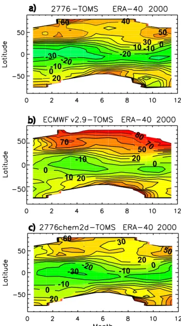
Fig. 8.Total O3column differences (DU) with respect to TOMS for SLIMCAT runs using(a)the COPCAT scheme,(b)the ECMWF v2.9 scheme and(c)the COPCAT scheme with the CHEM2Df¯
climatology (see text in Sect. 1 for details). Simulations use ERA-40 winds for year 2000. Contour interval is 10 DU. Colours range from dark green (most negative difference) to red (most positive difference).
Previous studies using the FK98 in place of the O3 refer-ence term include Eskes et al. (2003), where the FK98 clima-tology was used instead of the default term in the McLinden et al. (2000) parameterisation, to minimise conflicts within the data assimilation system (TM3DAM). However, no com-parison between both ozone reference terms (default and FK98) was provided. In McCormack et al. (2006) the FK98 climatology was used because it was the one used to initial-ize their model at upper levels, therefore, reducing additional biases. However, they did not compare results using different climatologies either. Geer et al. (2007) did show a compar-ison for the ECMWF v2.1 scheme using either the default supplied climatology term or the FK98 climatology. Their results suggested the existence of biases in the default cli-matology with respect to FK98. This agrees with the im-provements we find here when using the observation-based reference term. Geer et al. (2007) showed that, outside the polar night region, the climatologies are the main controlling factor for the upper stratosphere and mesosphere. In these regions the short photochemical lifetime of ozone causes a fast relaxation to the reference state. Our results agree with their findings in that the main influence of changing to the new climatology in our simulations is most evident above 10 hPa (e.g. as shown in Fig. 7). However, in our simulations we also find that changing the climatology affects the perfor-mance of the scheme over the Antarctic spring, which was not implied by the Geer et al. (2007) study.
4.2 Comparison versus ECMWF v2.9
Both COPCAT and the ECMWF scheme are based on the same linear CD approach although their treatment of hetero-geneous chemistry is very different. While COPCAT con-siders heterogeneous and gas-phase chemistry in a consis-tent way, the ECMWF scheme coefficients include only gas-phase chemistry and an additional term is used to model the heterogeneous chemistry effects over the poles. The COP-CAT scheme is here compared in detail with the current ECMWF operational scheme in SLIMCAT 3-D runs.
Figure 8 shows total O3 column differences between SLIMCAT runs using COPCAT and ECMWF ozone schemes and TOMS for year 2000. Over the tropics both schemes underestimate column values, COPCAT simulat-ing up to 30 DU less than observed and v2.9 up to 20 DU less. These differences are related to those in the under-estimation of the maximum in the tropical profiles shown in Fig. 7. Over northern mid and high latitudes the differ-ences are particularly large for the ECMWF scheme, which clearly overestimates column values compared to TOMS. In the Antarctic, both schemes overestimate TO column, except in October-December, when COPCAT underestimates ozone column values by 10–20 DU. Further comparisons at polar latitudes are discussed in Sect. 4.3.
Like COPCAT, the ECMWF scheme underestimates the tropical maximum with respect to full chemistry (Fig. 7).
Nevertheless, ECMWF ozone is∼1 ppmv larger than COP-CAT above 5 hPa. The annual mean zonal mean ECMWF O3 distribution (figure not shown) also confirms this; the ECMWF O3 maximum centred at 10 hPa is larger than in the COPCAT simulation for all latitudes, although lower than the full-chemistry run over tropics and mid-latitudes. At NH high latitudes (Fig. 6) the ECMWF scheme simulates too high O3in the mid/lower stratosphere compared to both the full-chemistry and COPCAT; up to 2 ppmv higher in June– July. The differences in the mid/lower stratosphere between ECMWF ozone and COPCAT or full-chemistry are larger in the Antarctic region. From September to November the ECMWF scheme in the LS (∼100 hPa) is larger than the SLIMCAT full-chemistry or the COPCAT parameterisation (lower panel in Fig. 6). This helps to explain why the ozone hole is not as deep with the ECMWF scheme as it is with COPCAT or SLIMCAT full-chemistry (Fig. 8 and Sect. 4.3). Vertical features above 100 hPa also differ, with ECMWF O3 being larger overall and showing too fast a recovery of the O3 hole, similar to COPCAT, compared to the full-chemistry.
As shown in Fig. 7, the use of a different O3 climatol-ogy changed COPCAT tropical profiles above 10 hPa. There-fore, at low latitudes the different reference state f¯ used in the ECMWF and COPCAT schemes might be playing the fundamental role in explaining the differences between both schemes. At high latitudes, the different heterogeneous chemistry treatment is the most probable cause of discrep-ancy between the schemes. However, at mid-latitudes both factors play important roles and it is difficult to attribute the main cause of the differences.
4.3 Polar winter/spring O3with COPCAT
This section compares the ability of the COPCAT scheme to simulate O3destruction at high latitudes with that of the full-chemistry CTM and the ECMWF scheme including the heterogeneous term in Eq. (1). It also shows the ability of COPCAT to adapt to different meteorological conditions (cold/warm polar winters).
Figure 9a and b show TO column January–December 2000 at 85◦N and 75◦N, respectively, for SLIMCAT simulations
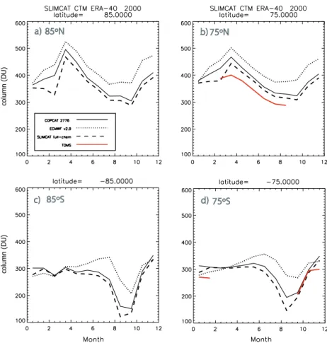
using the COPCAT scheme, the ECMWF scheme and the full-chemistry. The two parameterisations result in too large column values compared to the full-chemistry and TOMS. The ECMWF scheme results in the highest column val-ues, 30 DU higher than COPCAT on average over high NH latitudes and ∼80 DU higher than TOMS at 75◦N. In the
Antarctic COPCAT column values are very close to full-chemistry (Fig. 9c and d). The ozone hole in September– October is better represented by COPCAT than by the ECMWF scheme which, except for the summer months, re-sults in column values much larger than the other two runs (full-chemistry and COPCAT). Based on the few TOMS observations available at 75◦S both COPCAT and
a)
c)
b)
d)
85ºS 75ºS
85ºN 75ºN
col
umn
(DU)
col
umn
(DU)
Fig. 9. Total ozone column (DU) zonally averaged time series January–December 2000 at(a)85◦N,(b)75◦N,(c)85◦S and(d)75◦S.
Results are from SLIMCAT simulations using ERA-40 winds for COPCAT (solid line), ECMWF v2.9 (dotted line) and full-chemistry (dashed line). TOMS data are also included at 75◦N and 75◦S from spring to autumn (red line).
than 5 DU for the available observations during September-October. These results are a further proof of the suitabil-ity of the implicit heterogeneous chemistry approach. The high column values obtained with the ECMWF scheme in the Antarctic region during winter (Fig. 9c and d) can in part be explained by transport of ozone from higher altitudes. In the Antarctic region the ECMWF scheme concentrations above 50 hPa are significantly larger than for the COPCAT scheme and the full chemistry for winter months (Fig. 6). The descent of air masses carrying such higher concentra-tions contributes to the increase in the total column during winter shown with the ECMWF scheme (Fig. 9c). Although the rate of decrease for the period of sharp ozone decline is similar for both schemes, the COPCAT scheme, as well as the full-chemistry run, already starts to show some decline in late winter due to the ongoing loss at the edge of the vortex; this loss process is missed by the heterogeneous treatment in the current ECMWF scheme. The implicit calculation ap-proach in the new COPCAT scheme makes it less vulnerable to transport problems and able to achieve realistic chemical loss at the edge of the polar vortex.
a)
b)
c) f )
d)
e)
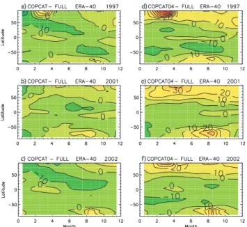
Fig. 10. Differences for the zonally averaged total ozone col-umn (DU) on the 15th of each month between COPCAT and full-chemistry run 323 for(a)1997,(b)2001 and(c)2002. Panels(d), (e)and(f)show differences between COPCAT04 and full-chemistry for the same years. Contour intervals are 10 DU. Colours range from dark green (most negative difference) to red (most positive difference).
regions COPCAT columns are 0–10 DU smaller than in the full-chemistry, over high latitudes the parameterisation gives larger column values than the full chemistry, but in no case are these differences larger than 10 DU. This situation is rep-resentative of what happens in other warm winters, e.g. 1992 or 1994 (not shown), while for 1999 (warm winter) the Arc-tic column values are up to 40 DU lower with the param-eterisation. So, for cold winters the COPCAT parameteri-sation tends to overestimate TO column (i.e. underestimate chemical loss) in the Arctic winter, while for most warm win-ters it provides values in very good agreement with the full-chemistry SLIMCAT (1999 being the only exception where the parameterisation destroys more O3 than the full chem-istry).
The poorer performance of the COPCAT scheme during cold Arctic winters can be explained by the fact that the co-efficients for the COPCAT parameterisation, like for all pre-vious linear ozone schemes, were calculated for the 15th of each month. And coefficients on the 15th March/September do not provide realistic loss rates for the sunlight levels found later in the month in the polar regions. This becomes more evident during cold winters, when the air processing inside the vortex has been more pronounced. Also, to calculate the coefficients, zonal mean output from the 3-D full-chemistry model was used, and coefficients were provided for every altitude/latitude (again as for previous existing schemes). Therefore, as longitudinal variability is not completely sim-ulated, features at the edge of the polar vortex will be
ne-glected. This will especially affect Arctic winters, as vortex breaking and filamentation events are more frequent than in the Antarctic.
To further show the sensitivity to the meteorology used to derive the coefficients (Sect. 4.1.2), Fig. 10d–f, show the differences between COPCAT04 and the full-chemistry, for same years as Fig. 10a–c. In this case, although the agree-ment with the full-chemistry is also very reasonable, the use of the COPCAT04 coefficients results in weaker polar loss compared to the default COPCAT. This shows that deriv-ing the scheme coefficients under cold winter meteorologi-cal conditions improves performance for cold winter years, without limiting the adaptability of the scheme for warmer winters.
Vertical profiles at 84◦N are shown in Fig. 11 for January–
July 1997, 2001 and 2002. It can clearly be seen how COP-CAT is able to follow well the full-chemistry variations in the three years. For the cold 1997 winter COPCAT shows a small underestimation in the middle stratosphere with re-spect to the full chemistry run, while for the warm 2001 win-ter the agreement is very good at least up to 10 hPa. In 2002 COPCAT exhibits a similar behaviour to that in 2001, except in March when COPCAT and the full-chemistry ozone field agree much better in 2002. The ECMWF v2.9 scheme tends to underestimate O3concentrations in the LS (∼0.25 ppmv) and to overestimate concentrations above 60 hPa by up to 2 ppmv, the overestimation being more obvious during the early months of winter (January–February). While these dif-ferences with the full chemistry are common to both the cold and warm winters, overall the ECMWF scheme is closer to the full chemistry profile during warm winter conditions than it is during colder winters.
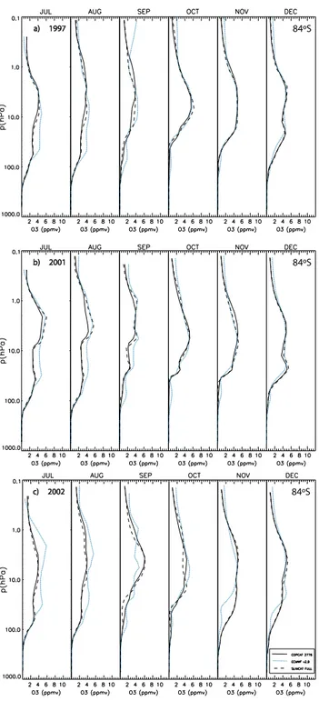
Even if warm and cold winter conditions do not affect the Antarctic as much as the Arctic it is also interesting to check the ability of COPCAT to simulate Antarctic O3loss for con-ditions different from year 2000 and, in particular, the ability of the new scheme to adapt to conditions such as those corre-sponding to the major warming detected in 2002. Figure 12 represents the O3vertical profiles from the COPCAT run, to-gether with the full-chemistry and the ECMWF scheme, for July–December 1997, 2001 and 2002 at 84◦S. These profiles
84ºN
84ºN
b) 2001 a) 1997
c) 2002 84ºN
Fig. 11. Zonally averaged vertical profiles of ozone (ppmv) on the 15th of each month at 84◦N for COPCAT (solid black), full-chemistry run 323 (dashed black) and ECMWF scheme (dotted blue). The period represented is January–July for the years(a) 1997,(b)2001 and(c)2002.
5 Summary
This work has tested the current ECMWF O3 parameteri-sation in a 3-D CTM, and suggested improvements for the current operational scheme. An alternative scheme has been
84ºS b) 2001
84ºS a) 1997
84ºS
c) 2002
Fig. 12. Zonally averaged vertical profiles of ozone (ppmv) on the 15th of each month at 84◦S for COPCAT (solid black), full-chemistry (dashed black) and ECMWF scheme (dotted blue). The period represented is July–December for the years (a)1997, (b) 2001 and(c)2002.
has been presented as a suitable improvement for schemes based on the linear Cariolle and D´equ´e approach, such as the operational ECMWF scheme.
The new linear ozone scheme has been obtained from SLIMCAT full-chemistry runs and for the first time it has been possible to compare a scheme of this kind with the full chemistry 3-D CTM used to calculate it. This has allowed the isolation of chemistry differences from other factors, such as numerics, resolution or transport. Obtaining a param-eterisation based on a widely tested CTM like SLIMCAT is crucial to evaluate and understand differences between the parameterisation and full-chemistry models. Moreover, the approach adopted here ensures that the parameterisa-tion obtained is as close as possible to a state-of-the-art full-chemistry CTM. COPCAT is in good overall agreement with SLIMCAT full-chemistry, although a significant reduction in the tropical maximum O3at 10 hPa occurs when using the parameterisation. A similar reduction takes place when us-ing the ECMWF scheme in a SLIMCAT run, which identi-fies a drawback of this kind of scheme with respect to full-chemistry models. Results have also shown the relevance of the choice of the reference state (climatology); using the Fortuin and Kelder (1998) O3climatology the tropical differ-ences against observations have been reduced for COPCAT runs.
The heterogeneous treatment adopted by COPCAT has provided the scheme with a realistic polar loss simulation showing that the linearisation approach can cope adequately with polar chemical processes. The new scheme is able to re-produce a realistic Antarctic ozone hole, and also over north-ern high latitudes COPCAT is more realistic than the current ECMWF scheme. Both treatments involve approximations, however, COPCAT has shown that heterogeneous chemistry can be included in the parameterisation consistently with the rest of the chemistry, without any additional tunable parame-ter. This approach has made COPCAT, not only more consis-tent with the full-chemistry, but also more adaptable to differ-ent atmospheric conditions. As shown in Sect. 4.3 COPCAT is able to reproduce the behaviour of the full chemistry model in the Arctic for both warm and cold winters.
It has also been shown that COPCAT is able to adapt to the unusual stratospheric meteorological patterns detected over Antarctica in 2002. The adaptability of the scheme makes it a good candidate to be used in the production of a long reanalysis series. Coefficients would only have to be recom-puted for periods in which atmospheric chemistry conditions were very different from present ones, mainly in terms of ozone depleting substances (ODS) concentrations. To adjust the tendencies to the actual chemistry conditions coefficients would be recomputed for years before 1980, when ODS con-centrations were still low enough not to produce ozone de-struction during the Antarctic spring, and again before the 1960s, when no significant ODS concentrations were present in the atmosphere (WMO, 2007).
The inclusion of heterogeneous chemistry in the scheme has not been detrimental for the linearity of the approach. Only at polar latitudes is the range of temperatures for the linear approximation somewhat restricted. Such temperature range (±10 K from the reference state) is still within the typ-ical variation range observed in global models (e.g. Shine et al., 2003), however, to ensure the accuracy of the scheme under all possible polar vortex conditions higher order terms could be included as a future improvement to the scheme. This would not increase much the cost of the scheme, as it would only mean the coefficients files to be read-in would contain more data. Based on the underestimation of polar loss by the linear parameterisations, coefficients could be provided twice a month, instead of just on the 15th of each month, to provide more realistic loss rates for the sunlight levels found in the polar early spring.
Other improvements that can easily be implemented in fu-ture COPCAT versions are the use of a higher vertical reso-lution, as well as basing the scheme in a full-chemistry run using the recent ERA-Interim reanalyses, which have already shown to provide more realistic results in the stratosphere than ERA-40 (e.g. Monge-Sanz et al., 2007). Solar cycle in-fluences could also be included in future COPCAT versions. Moreover, as the full chemistry SLIMCAT model is con-tinuously subject to revisions and improvements, following versions of COPCAT would benefit from the same develop-ments included in the CTM.
This study has also shown the sensitivity of this kind of linear scheme to the meteorology used to derive the coeffi-cients. Thus, care must be taken to choose those meteorolog-ical conditions that maximise the adaptability of the scheme to reproduce realistic polar loss under different polar win-ter conditions. We have compared coefficients derived under year 2000 meteorology (COPCAT) and a second version rived under year 2004 meteorology (COPCAT04). The de-fault COPCAT (based on year 2000 conditions) has shown better agreement with the full-chemistry than COPCAT04 and very good adaptability for a multiannual run.
The good agreement COPCAT presents with SLIMCAT full-chemistry is encouraging and shows the scheme as a promising alternative to the use of parameterisations with a separate treatment of gas-phase and heterogeneous chem-istry. Furthermore, given the good agreement between COP-CAT, the parent full-chemistry CTM and observations, a scheme like COPCAT can be used to assess the performance of two-way coupled systems including full-chemistry within a NWP model, e.g. the coupled system used by Flemming et al. (2010).
used in NWP and data assimilation systems, such as those of UK Met-Office, ECMWF or M´et´eo-France.
Acknowledgements. Authors are very grateful to Adrian Simmons
for useful discussions and support throughout this work. We also thank John McCormack for providing the CHEM2D coefficients and Agathe Untch, Elias H´olm and Rossana Dragani for many valuable communications on the ECMWF O3 scheme. We are also grateful to Alan Geer and one anonymous referee for their constructive reviews of the original manuscript. This work has been partially funded by the NERC Research Award NE/F004575/1.
Edited by: W. Lahoz
References
Bhatt, P. P., Remsberg, E. E., Gordley, L. L., McInerney, M. J., Brackett, V. G., and Russell III, J. M.: An evaluation of the quality of Halogen Occultation Experiment ozone profiles in the lower stratosphere, J. Geophys. Res., 104, 9261–9275, 1999. Br¨uhl, C., Drayson, S. R., Russell III, J. M., Crutzen, P. J.,
Mclner-ney, J. M., Purcell, P. N., Claude, H., Gernandt, H., McGee, T. J., McDermid, I. S., and Gunson, M. R.: Halogen Occulta-tion Experiment ozone channel validaOcculta-tion, J. Geophys. Res., 101, 10217–10240, 1996.
Cariolle, D. and D´equ´e, M.: Southern Hemisphere Medium-Scale Waves and Total Ozone Disturbances in a Spectral General Cir-culation Model, J. Geophys. Res., 91, 10825–10846, 1986. Cariolle, D. and Teyss`edre, H.: A revised linear ozone
photochem-istry parameterization for use in transport and general circula-tion models: multi-annual simulacircula-tions, Atmos. Chem. Phys., 7, 2183–2196, doi:10.5194/acp-7-2183-2007, 2007.
Carslaw, K. S., Luo, B. P., Clegg, S. L., Peter, T., Brimblecombe, P., and Crutzen, P. J.: Stratospheric aerosol growth and HNO3gas phase depletion from coupled HNO3and water uptake by liquid particles, Geophys. Res. Lett., 21, 2479–2482, 1994.
Chipperfield, M. P.: Multiannual simulations with a three-dimensional chemical transport model, J. Geophys. Res., 104, 1781–1805, 1999.
Chipperfield, M. P.: A three-dimensional model study of long-term mid-high latitude lower stratosphere ozone changes, At-mos. Chem. Phys., 3, 1253–1265, doi:10.5194/acp-3-1253-2003, 2003.
Chipperfield, M. P.: New version of the TOMCAT/SLIMCAT off-line chemical transport model, Q. J. Roy. Meteorol. Soc., 132, 1179–1203, doi:10.1256/qj.05.51, 2006.
Chipperfield, M. P., Cariolle, D., and Simon, P.: A 3-Dimensional transport model study of PSC processing during EASOE, Geo-phys. Res. Lett., 21, 1463–1466, 1994.
Chipperfield, M. P., Khattatov, B. V., and Lary, D. J.: Sequen-tial assimilation of stratospheric chemical observations in a three-dimensional model, J. Geophys. Res., 107(D21), 4585, doi:10.1029/2002JD002110, 2002.
Dethof, A.: Aspects of modelling and assimilation for the strato-sphere at ECMWF, SPARC Newsletter, 21, 2003.
Dethof, A. and H´olm, E. V.: Ozone assimilation in the ERA-40 reanalysis project, Q. J. Roy. Meteorol. Soc., 130, 2851–2872, 2004.
Eskes, H. J., Van Velthoven, P. F. J., Valks, P. J. M., and Kelder, H. M.: Assimilation of GOME total-ozone satellite observations in a three-dimensional tracer-transport model, Q. J. Roy. Meteo-rol. Soc., 129, 1663–1681, 2003.
Eyring, V., Butchart, N., Waugh, D. W., Akiyoshi, H., Austin, J., Bekki, S., Bodeker, G. E., Boville, B. A., Br¨uhl, C., Chipper-field, M. P., Cordero, E., Dameris, M., Deushi, M., Fioletov, V. E., Frith, S. M., Garcia, R. R., Gettelman, A., Giorgetta, M. A., Grewe, V., Jourdain, L., Kinnison, D. E., Mancini, E., Manzini, E., Marchand, M., Marsh, D. R., Nagashima, T., Newman, P. A., Nielsen, J. E., Pawson, S., Pitari, G., Plummer, D. A., Rozanov, E., Schraner, M., Shepherd, T. G., Shibata, K., Stolarski, R. S., Struthers, H., Tian, W., and Yoshiki, M.: Assessment of tem-perature, trace species, and ozone in chemistry-climate model simulations of the recent past, J. Geophys. Res., 111, D22308, doi:10.1029/2006JD007327, 2006.
Feng, W., Chipperfield, M. P., Dorf, M., Pfeilsticker, K., and Ri-caud, P.: Mid-latitude ozone changes: studies with a 3-D CTM forced by ERA-40 analyses, Atmos. Chem. Phys., 7, 2357–2369, doi:10.5194/acp-7-2357-2007, 2007.
Flemming, J., Inness, A., Jones, L., Eskes, H. J., Huijnen, V., Schultz, M. G., Stein, O., Cariolle, D., Kinnison, D., and Brasseur, G.: Forecasts and assimilation experiments of the Antarctic Ozone Hole 2008, Atmos. Chem. Phys. Discuss., 10, 9173–9217, doi:10.5194/acpd–10–9173–2010, 2010.
Fortuin, J. P. F. and Kelder, H.: An ozone climatology based on ozonesonde and satellite measurements, J. Geophys. Res., 103, 31709–31734, 1998.
Geer, A. J., Lahoz, W. A., Jackson, D. R., Cariolle, D., and McCormack, J. P.: Evaluation of linear ozone photochemistry parametrizations in a stratosphere-troposphere data assimilation system, Atmos. Chem. Phys., 7, 939–959, doi:10.5194/acp-7-939-2007, 2007.
Hanson, D. and Mauersberger, K.: Laboratory studies of the ni-tric acid trihydrate: Implications for the South Polar stratosphere, Geophys. Res. Lett., 15, 855–858, 1988.
Manney, G. L., Krueger, K., Sabutis, J. L., Sena, S. A., and Paw-son, S.: The remarkable 2003-2004 winter and other recent warm winters in the Arctic stratosphere since the late 1990s, J. Geo-phys. Res., 110, D04107, doi:10.1029/2004JD005 367, 2005. McCormack, J. P., Eckermann, S. D., Coy, L., Allen, D. R., Kim,
Y.-J., Hogan, T., Lawrence, B., Stephens, A., Browell, E. V., Burris, J., McGee, T., and Trepte, C. R.: NOGAPS-ALPHA model sim-ulations of stratospheric ozone during the SOLVE2 campaign, Atmos. Chem. Phys., 4, 2401–2423, doi:10.5194/acp-4-2401-2004, 2004.
McCormack, J. P., Eckermann, S. D., Siskind, D. E., and McGee, T. J.: CHEM2D-OPP: A new linearized gas-phase ozone pho-tochemistry parameterization for high-altitude NWP and climate models, Atmos. Chem. Phys., 6, 4943–4972, doi:10.5194/acp-6-4943-2006, 2006.
McHugh, M., Magill, B., K. A. Walker, C. D. B., Bernath, P. F., and Russell III, J. M.: Comparison of atmospheric retrievals from ACE and HALOE, Geophys. Res. Lett., 32, L15S10, doi:10.1029/2005GL022 403, 2005.
McPeters, R., Bhartia, P., Krueger, A., Herman, J. R., Wellemeyer, C., Seftor, C., Jaross, G., Torres, O., Moy, L., Labow, G., Byerly, W., Taylor, S., Swissler, T., and Cebula, R.: Earth Probe To-tal Ozone Mapping Spectrometer (TOMS) Data Products User’s Guide, NASA Ref. Publ. 206895, 1998.
Monge-Sanz, B. M.: Stratospheric Transport and Chemical Param-eterisations in ECMWF Analyses: Evaluation and Improvements using a 3-D CTM, Ph.D. thesis, Earth and Environment School, University of Leeds, UK, 2008.
Monge-Sanz, B. M., Chipperfield, M. P., Simmons, A. J., and Up-pala, S. M.: Mean age of air and transport in a CTM: Comparison of different ECMWF analyses, Geophys. Res. Lett., 34, L04801, doi:10.1029/2006GL028515, 2007.
Morris, G. A., Gleason, J. F., Russell III, J. M., Schoeberl, M. R., and McCormick, M. P.: A comparison of HALOE V19 with SAGE II V6.00 ozone observations using trajectory mapping, J. Geophys. Res., 107(D13), 4177, doi:10.1029/2001JD000847, 2002.
Newman, P. A. and Nash, E. R.: The Unusual Southern Hemi-sphere StratoHemi-sphere Winter of 2002, J. Atmos. Sci., 62, 614–628, doi:10.1175/JAS–3323.1, 2005.
Searle, K. R., Chipperfield, M. P., Bekki, S., and Pyle, J. A.: The impact of spatial averaging on calculated polar ozone loss 2. The-oretical analysis, J. Geophys. Res., 103, 25409–25416, 1998. Shine, K. P., Bourqui, M. S., de F. Forster, P. M., Hare, S. H. E.,
Langematz, U., Braesicke, P., Grewe, V., Ponater, M., Schnadt, C., Smith, C. A., Haigh, J. D., Austin, J., Butchart, N., Shindell, D. T., Randel, W. J., Nagashima, T., Portmann, R. W., Solomon, S., Seidel, D. J., Lanzante, J., Klein, S., Ramaswamy, V., and Schwarzkopf, M. D.: A comparison of model-simulated trends in stratospheric temperatures, Q. J. Roy. Meteorol. Soc., 129, 1565– 1588, doi:10.1256/qj.02.186, 2003.
Sinnhuber, B.-M, Chipperfield, M., Davies, S., Burrows, J., Eich-mann, K.-U., Weber, M., von der Gathen, P., Guirlet, M., Cahill, G. A., Lee, A., and Pyle, J. A.: Large loss of total ozone during the Arctic winter of 1999/2000, Geophys. Res. Lett., 27, 3473– 3476, 2000.
Steil, B., Br¨uhl, C., Manzini, E., Crutzen, P. J., Lelieveld, J., Rasch, P. J., Roeckner, E., , and Kr¨uger, K.: A new interactive chemistry-climate model: 1. Present-day climatology and inter-annual variability of the middle atmosphere using the model and 9 years of HALOE/UARS data, J. Geophys. Res., 108(D9), 4290, doi:10.1029/2002JD002971, 2003.
Uppala, S. M., K˚allberg, P. W., Simmons, A. J., Andrae, U., Bech-told, V. D. C., Fiorino, M., Gibson, J. K., Haseler, J., Hernandez, A., Kelly, G. A., Li, X., Onogi, K., Saarinen, S., Sokka, N., Al-lan, R. P., Andersson, E., Arpe, K., Balmaseda, M. A., Beljaars, A. C. M., Berg, L. V. D., Bidlot, J., Bormann, N., Caires, S., Chevallier, F., Dethof, A., Dragosavac, M., Fisher, M., Fuentes, M., Hagemann, S., H´olm, E., Hoskins, B. J., Isaksen, L., Janssen, P. A. E. M., Jenne, R., Mcnally, A. P., Mahfouf, J.-F., Morcrette, J.-J., Rayner, N. A., Saunders, R. W., Simon, P., Sterl, A., Tren-berth, K. E., Untch, A., Vasiljevic, D., Viterbo, P., and Woollen, J.: The ERA-40 Re-analysis, Q. J. Roy. Meteorol. Soc., 131, 2961–3012, doi:10.1256/qj.04.176, 2005.