ACPD
14, 12323–12375, 2014Satellite observations of cirrus clouds in the Northern Hemisphere
R. Spang et al.
Title Page
Abstract Introduction
Conclusions References
Tables Figures
◭ ◮
◭ ◮
Back Close
Full Screen / Esc
Printer-friendly Version
Interactive Discussion
Discussion
P
a
per
|
D
iscussion
P
a
per
|
Discussion
P
a
per
|
Discuss
ion
P
a
per
|
Atmos. Chem. Phys. Discuss., 14, 12323–12375, 2014 www.atmos-chem-phys-discuss.net/14/12323/2014/ doi:10.5194/acpd-14-12323-2014
© Author(s) 2014. CC Attribution 3.0 License.
Atmospheric Chemistry and Physics
Open Access
Discussions
This discussion paper is/has been under review for the journal Atmospheric Chemistry and Physics (ACP). Please refer to the corresponding final paper in ACP if available.
Satellite observations of cirrus clouds in
the Northern Hemisphere lowermost
stratosphere
R. Spang1, G. Günther1, M. Riese1, L. Hoffmann2, R. Müller1, and S. Griessbach2
1
Forschungszentrum Jülich, Institut für Energie and Klimaforschung, IEK-7, Jülich, Germany
2
Forschungszentrum Jülich, Jülich Supercomputing Centre, JSC, Jülich, Germany
Received: 24 March 2014 – Accepted: 26 April 2014 – Published: 14 May 2014
Correspondence to: R. Spang ([email protected])
ACPD
14, 12323–12375, 2014Satellite observations of cirrus clouds in the Northern Hemisphere
R. Spang et al.
Title Page
Abstract Introduction
Conclusions References
Tables Figures
◭ ◮
◭ ◮
Back Close
Full Screen / Esc
Printer-friendly Version
Interactive Discussion
Discussion
P
a
per
|
D
iscussion
P
a
per
|
Discussion
P
a
per
|
Discuss
ion
P
a
per
|
Abstract
Here we present observations of the Cryogenic Infrared Spectrometers and Telescopes for the Atmosphere (CRISTA) of cirrus cloud and water vapour in August 1997 in the upper troposphere and lower stratosphere (UTLS) region. The observations indicate a considerable flux of moisture from the upper tropical troposphere into the
extra-5
tropical lowermost stratosphere (LMS), resulting in the occurrence of high altitude op-tically thin cirrus clouds in the LMS.
The locations of the LMS cloud events observed by CRISTA are consistent with the tropopause height determined from coinciding radiosonde data. For a hemispheric analysis in tropopause relative coordinates an improved tropopause determination has
10
been applied to the ECMWF temperature profiles. We found that a significant fraction of the cloud occurrences in the tropopause region are located in the LMS, even if a conservative overestimate of the cloud top height (CTH) determination by CRISTA of 500 m is assumed. The results show rather high occurrence frequencies (∼5 %) up to high northern latitudes (70◦N) and altitudes well above the tropopause (>500 m at
15
∼350 K and above) in large areas at mid and high latitudes.
Comparisons with model runs of the Chemical Lagragian Model of the Stratosphere (CLaMS) over the CRISTA period show a reasonable consistency for the retrieved cloud pattern. For this purpose a limb ray tracing approach was applied through the 3-D model fields to obtain integrated measurement information through the atmosphere
20
along the limb path of the instrument. The simplified cirrus scheme implemented in CLaMS seems to cause a systematic underestimation in the CTH occurrence frequen-cies in the LMS with respect to the observations. The observations together with the model results demonstrate the importance of isentropic, quasi-horizontal transport of water vapour from the sub-tropics and the potential for the occurrence of cirrus clouds
25
ACPD
14, 12323–12375, 2014Satellite observations of cirrus clouds in the Northern Hemisphere
R. Spang et al.
Title Page
Abstract Introduction
Conclusions References
Tables Figures
◭ ◮
◭ ◮
Back Close
Full Screen / Esc
Printer-friendly Version
Interactive Discussion
Discussion
P
a
per
|
D
iscussion
P
a
per
|
Discussion
P
a
per
|
Discuss
ion
P
a
per
|
1 Introduction
A large proportion of the uncertainties of climate change projections by general circu-lation models (GCMs) arises from poorly understood and represented interactions and feedbacks between dynamic, microphysical, and radiative processes affecting cirrus
clouds (IPCC, 2014). Modelled climates are sensitive even to small changes in cirrus
5
coverage or ice microphysics (Kärcher and Spichtinger, 2010). Fusina et al. (2007) point out that the net radiative impact strongly depends on ice water content and ice crystal number concentration. Small changes in the effective radius of the size
distribu-tions can substantially modify the surface temperatures.
Recent GCM studies (Sanderson et al., 2008; Mitchell et al., 2008) indicate that the
10
climate impact of cirrus clouds depends in particular on the fall speed of ice particles, which in turn depends on ice nucleation rates (i.e. the concentrations of small ice crys-tals). The overall net warming effect of cirrus clouds can be substantially reduced by
changing the concentrations of small ice crystals (i.e. the degree of bimodality) of the particle size distribution (PSD). The size distribution strongly affects the representative 15
PSD ice fall speed. Mitchell and Finnegan (2009) investigated this sensitivity in more detail and concluded that cirrus clouds are a logical candidate for climate modification efforts.
The large uncertainties in climate prediction caused by processes involving cirrus clouds highlight the importance of more quantitative information on cirrus clouds by
20
observations, especially for optically thin and small particle cirrus clouds like contrails close to the tropopause, which may have an overall cooling effect in contradiction to
lower cirrus (Zhang et al., 2005). However, uncertainties for the climate feedback of cirrus clouds are still very large and a substantial reduction is needed (IPCC, 2014).
In particular, the altitude region of the Upper Troposphere and Lower Stratosphere
25
ACPD
14, 12323–12375, 2014Satellite observations of cirrus clouds in the Northern Hemisphere
R. Spang et al.
Title Page
Abstract Introduction
Conclusions References
Tables Figures
◭ ◮
◭ ◮
Back Close
Full Screen / Esc
Printer-friendly Version
Interactive Discussion
Discussion
P
a
per
|
D
iscussion
P
a
per
|
Discussion
P
a
per
|
Discuss
ion
P
a
per
|
concentrations of water vapour (H2O) have significant effects on the atmospheric
radi-ation balance (e.g. Solomon et al., 2010; Riese et al., 2012).
Detailed understanding and modelling of the transport pathways of water vapour, and consequently the realistic representation of total water (gaseous and condensed form) in the UTLS region are therefore crucial for the correct representation of clouds
5
and water vapour in climate models. Comprehensive analyses are published on trans-port processes from the troposphere into the stratosphere and tracer protrans-portions of the extra-tropical UTLS region (e.g. Hegglin et al., 2009; Hoor et al., 2010; Ploeger et al., 2013). Rossby wave breaking (Ploeger et al., 2013) and mid-latitude overshoot convec-tion (Dessler, 2009) result in transport and mixing of air masses into the extra-tropical
10
UTLS on short time scales (weeks). On seasonal time scales, downwelling by the deep Brewer–Dobson circulation branch moistens the extra-tropical UTLS at altitudes above 450 K (Ploeger et al., 2013). Aged air masses transported into the extra-tropical lower stratosphere from above are moistened by methane oxidation and represent an impor-tant source for water vapour in the middle stratosphere (e.g., Jones and Pyle, 1984;
15
Rohs et al., 2006).
The imprint of various water vapour transport ways into the lowermost stratosphere on cirrus formation has been investigated in a limited number of studies (Dessler, 2009; Montaux et al., 2010; Pan and Munchak, 2011; Wang and Dessler, 2012). The forma-tion of cirrus clouds above the mid-latitude tropopause is discussed so far quite
contro-20
versially. Dessler (2009) found relatively high occurrence rates of cirrus above the mid and high latitude tropopause in space borne lidar data of the Cloud and Aerosol Lidar (CALIOP) instrument on the Cloud Aerosol Lidar Infrared Pathfinder Satellite Observa-tions (CALIPSO) (Winker et al., 2010). The analysis of Dessler (2009) shows cloud top height occurrences above the tropopause of up to 30–40 % for mid-high and tropical
25
ACPD
14, 12323–12375, 2014Satellite observations of cirrus clouds in the Northern Hemisphere
R. Spang et al.
Title Page
Abstract Introduction
Conclusions References
Tables Figures
◭ ◮
◭ ◮
Back Close
Full Screen / Esc
Printer-friendly Version
Interactive Discussion
Discussion
P
a
per
|
D
iscussion
P
a
per
|
Discussion
P
a
per
|
Discuss
ion
P
a
per
|
measurements. They find substantially fewer clouds above the tropopause and in their analysis the CALIOP data do not provide sufficient evidence of significant presence of
cirrus clouds above the mid-latitude tropopause. The remaining but evidential events in the tropics show occurrences up to 24 % in the western Pacific and are usually located between the cold point and the lapse rate tropopause (up to 2.5 km above). PM2011
5
speculated that most of these clouds are triggered by gravity wave induced temper-ature disturbances, which typically are observed above deep convection areas (e.g. Hoffmann and Alexander, 2010).
In contrast, cloud observations by mid-latitude lidar stations show frequent events at and above the tropopause (e.g. Keckhut et al., 2005; Rolf, 2013). Many of them coincide
10
with the observations of a secondary tropopause (Noël and Haeffelin, 2007). Isentropic
transport and mixing of subtropical air masses with tropospheric high water values into the mid-latitude and polar LMS may cause such events and Montaux et al. (2010), in a case study, were able to reproduce the observation of such a cloud with an isentropic transport model by implementing a simple microsphysical cloud model. However in
15
this study, the cloud was observed just at the tropopause and not significantly above. Eixmann et al. (2010) investigated the dynamical link between poleward Rossby wave breaking (RWB) events and the occurrence of upper tropospheric cirrus clouds for lidar measurements above Kühlungsborn (54.1◦N, 11.8◦E). For three similar cirrus events they found a strong link between low values of potential vorticity (a proxy for RWB
20
activity), enhanced up-draft velocities, and cloud ice water content. They concluded that based on the climatology of poleward RWB events following the method of Gabriel and Peters (2008) a parameterisation of the formation or occurrence of high and thin cirrus clouds seems to be possible.
Although there are a couple of ground based lidar observations suggesting the
pres-25
ACPD
14, 12323–12375, 2014Satellite observations of cirrus clouds in the Northern Hemisphere
R. Spang et al.
Title Page
Abstract Introduction
Conclusions References
Tables Figures
◭ ◮
◭ ◮
Back Close
Full Screen / Esc
Printer-friendly Version
Interactive Discussion
Discussion
P
a
per
|
D
iscussion
P
a
per
|
Discussion
P
a
per
|
Discuss
ion
P
a
per
|
frequently do these cirrus clouds occur on global scales, and are clouds tops or even complete clouds significantly above the tropopause.
The currently most sensitive sensor in space for cirrus cloud observations is the CALIOP lidar. Nonetheless, Davis et al. (2010) pointed out that the space lidar on CALIPSO might miss 2/3 of thin cirrus clouds with vertically optical depthτ <0.01 in
5
its current data products. Clouds with such a very low optically thicknesses have been observed by airborne lidars and in-situ instruments in the validation campaigns for CALIPSO. Frequently these cloud layers showed IWC values smaller than 10−5g m−3 (Davis et al., 2010).
Here we argue that IR limb sounding from space provide an alternative
measure-10
ment technique of high sensitivity for the detection of optically thin clouds (Mergen-thaler et al., 1999; Spang et al., 2002; Massie et al., 2007; Griessbach et al., 2013), subvisible cirrus (SVC) defined by the extinction range 2×10⁻⁴–2×10⁻²km−1(Sassen et al., 1989), or the even thinner ultra-thin tropical cirrus (UTTC) (Peter et al., 2003; Luo et al., 2003). The detection sensitivity for clouds of IR limb sounders is in the range of
15
spaceborne lidar measurements (Höpfner et al., 2009; Spang et al., 2012). A 100 km or even 1 km horizontally extended cirrus cloud is detectable by an IR limb sounder with an ice water content (IWC) of 3×10⁻⁶ and 3×10⁻⁴g m−3 respectively (Spang et al., 2012), presupposed that the cloud fills completely the field of view of the instrument. These values represent even better detection sensitivity than the current CALIOP cloud
20
products.
In this paper we like to present new analyses of measurements from the Cryo-genic Infrared Spectrometers and Telescopes for the Atmosphere (CRISTA) instrument during its 2nd Space Shuttle mission in August 1997 (CRISTA-2) (Grossmann et al., 2002). Due to its unique combination of moderate spectral resolution, high horizontal
25
ACPD
14, 12323–12375, 2014Satellite observations of cirrus clouds in the Northern Hemisphere
R. Spang et al.
Title Page
Abstract Introduction
Conclusions References
Tables Figures
◭ ◮
◭ ◮
Back Close
Full Screen / Esc
Printer-friendly Version
Interactive Discussion
Discussion
P
a
per
|
D
iscussion
P
a
per
|
Discussion
P
a
per
|
Discuss
ion
P
a
per
|
nadir passive and active instruments as well as limb sounders in the uv-vis and mi-crowave wavelength region. The characterisation of frequent observations of Northern Hemisphere mid- and high-latitude cirrus clouds in respect to the tropopause (above or below) are in the focus of the present study.
The paper is organised as follows. First we introduce the CRISTA instrument and
5
the applied data analysis methods followed by a section presenting the cloud top oc-currence frequencies (COF) in respect to the tropopause. The comparison of CRISTA water vapour and cloud measurements presented in Sect. 4 is suggesting a strong in-fluence of horizontal transport processes of high water vapour values from the subtrop-ics to the latitude of cloud formation. A comparison with a global transport model can
10
help to understand the origin and evolution with time of the cloud observations around the tropopause. This is investigated in Sect. 5 with a Lagrangian transport model con-taining a simple cirrus parameterisation.
2 Observations and analysis methods
2.1 CRISTA satellite instrument
15
The Cryogenic Infrared Spectrometers and Telescopes for the Atmosphere (CRISTA) instrument measured roughly one week in the UTLS during two space shuttle mis-sions in November 1994 and August 1997 (Offermann et al., 1999; Grossmann et al.,
2002). The measurements demonstrate the potential of the IR limb viewing technique to provide information on several trace gas constituents (Riese et al., 1999a, 2002) and
20
clouds (Spang et al., 2002) with high spatial resolution. The spectral information in the wavelength (λ) region 4–15 µm is scanned with a resolution of λ/∆λ=∼500, which is
equivalent to 1.6 cm−1at 830 cm−1. The vertical field of view (resolution) is in the order of 1.5 km and a typical vertical sampling of 2 km was used during CRISTA-2. A horizon-tal along-track sampling of 200 to 400 km was applied, depending on the measurement
25
ACPD
14, 12323–12375, 2014Satellite observations of cirrus clouds in the Northern Hemisphere
R. Spang et al.
Title Page
Abstract Introduction
Conclusions References
Tables Figures
◭ ◮
◭ ◮
Back Close
Full Screen / Esc
Printer-friendly Version
Interactive Discussion
Discussion
P
a
per
|
D
iscussion
P
a
per
|
Discussion
P
a
per
|
Discuss
ion
P
a
per
|
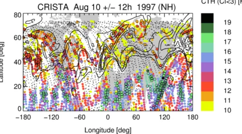
for three viewing directions simultaneously. A typical measurement net in the North-ern Hemisphere is illustrated in Fig. 1. Due to the overlapping orbits and the 57◦orbit inclination an even higher horizontal cross-track sampling becomes obvious at high northern latitudes (∼200 km for north of 60◦ latitude). The spectrometers and optics were cryogenically cooled by helium to allow for measurements in the middle and far
5
infra-red (4–70 µm).
The instrument was hosted by the free-flyer system ASTRO-SPAS (Wattenbach and Moritz, 1997). The accuracy of the attitude system of the platform which was also used for two astronomic missions is excellent. The final pointing accuracy in the limb direction for the three viewing directions is in the order of 300 m (Riese et al., 1999a;
10
Grossmann et al., 2002). The effect of refraction through the atmosphere in the limb
direction is considered in the tangent height determination and can reduce the actual tangent height by up to∼300 m at 12 km altitude. This correction is crucial for the cloud top height determination in the next section.
Here, we focus on the CRISTA-2 mission which took place from 8 to 15 August
15
in 1997. Details on the instrument, the mission, and the specific water vapour re-trieval are given in Grossmann et al. (2002); Offermann et al. (2002); and Schaeler
et al. (2005) respectively. For the water vapour retrieval the continuous spectral scans of the spectrometers allow the selection of a spectral water vapour feature most suit-able at tropopause altitudes (at a wavelength of 12.7 µm). An onion peeling retrieval is
20
applied to the CRISTA measurements (Riese et al., 1999; Schaeler and Riese, 2001) and has the advantage of no upward propagation of errors to altitudes levels above optically thick clouds, even if the spectrum is not removed from the retrieval. The con-tamination by the strong cloud emissions and scattering processes in the correspond-ing IR spectra are too complex to model accurately in the retrieval process, and these
25
ACPD
14, 12323–12375, 2014Satellite observations of cirrus clouds in the Northern Hemisphere
R. Spang et al.
Title Page
Abstract Introduction
Conclusions References
Tables Figures
◭ ◮
◭ ◮
Back Close
Full Screen / Esc
Printer-friendly Version
Interactive Discussion
Discussion
P
a
per
|
D
iscussion
P
a
per
|
Discussion
P
a
per
|
Discuss
ion
P
a
per
|
2.2 CRISTA cloud detection
In the following special emphasis is put on cloud top height (CTH) observations at NH mid-latitudes in respect to the tropopause, where isentropic horizontal transport of wa-ter vapour from the subtropics to high latitudes may trigger cirrus formation in LMS. The cloud detection for IR limb sounders has been investigated in detail over the last
5
decade (Spang et al., 2012, and references therein). For spectrally resolved measure-ments simple colour ratio based methods are shown to be robust and accurate for the detection of cloudy spectra (e.g. Spang et al., 2001; Sembhi et al., 2012). For the follow-ing analyses the cloud index (CI) is defined by the colour ratio of the mean radiances from 788 to 796 cm−1divided by the mean radiances from 832 to 834 cm−1, which was
10
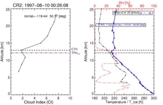
already applied to various airborne and spaceborne limb IR instruments (e.g. Spang et al., 2002, 2004, 2007). The corresponding CTH is the first tangent height where CI falls below the defined threshold value (CIthres). The left panel of Fig. 2 illustrates a CI profile with the transition from clear sky conditions (8>CI>4.5) to cloudy conditions (∼4>CI>1.1), where optically thick conditions are in line with a CI-value of∼1.2.
15
Various studies have shown that the detection sensitivity is linked to the detection threshold and depends to some extent on the seasonal variation in the trace gas con-centrations in the applied spectral windows (e.g. Spang et al., 2012). The main limiting effect of the cloud index method are high water vapour continuum emissions (for mixing
ratios>500 ppmv) in the mid troposphere and below. Under such conditions a definite
20
discrimination between clouds and high water becomes difficult (Spang et al., 2004,
2007).
Cloud top heights detected with a cloud index threshold value of CIthres=3 are pre-sented in Fig. 1. Inhomogeneities in the measurement net are caused by special mea-surement modes, where the free-flyer was pointed to specific regions of interest (e.g.
25
ACPD
14, 12323–12375, 2014Satellite observations of cirrus clouds in the Northern Hemisphere
R. Spang et al.
Title Page
Abstract Introduction
Conclusions References
Tables Figures
◭ ◮
◭ ◮
Back Close
Full Screen / Esc
Printer-friendly Version
Interactive Discussion
Discussion
P
a
per
|
D
iscussion
P
a
per
|
Discussion
P
a
per
|
Discuss
ion
P
a
per
|
streamers (e.g. Riese et al., 1999a, 2002) in conjunction with meteorological parame-ters like the potential vorticity (PV). Figure 1 shows PV contours for the 350 K isentrope. All meteorological data used in this study are from the ERA Interim reanalysis dataset provided by the European centre for medium-range weather forecasts (ECMWF) (Dee al., 2011). The CTH distribution and PV contours are suggesting a link between the
dy-5
namical features of horizontal transport processes like Rossby wave breaking events (e.g. Juckes and McIntyre, 1987) and the presence of high cirrus clouds. Contours of low PV (4 and 8 PVU, with 1 PVU=10−6K m2kg−1s−1) are highlighting elongated air
masses from the subtropics to mid and high latitudes where coincidently high altitude clouds appear in the CRISTA observations.
10
High CTHs (>12 km) are frequently present at mid (40–60◦N) and even at high geo-graphic latitudes (>60◦N) in regions of low PV. Nearly all of these high CTH locations show PV values greater 2 PVU, a common threshold for the dynamical tropopause in the subtropics (Holton et al., 1995), and marked in Fig. 2 by black circles. Whether these clouds are really formed in the LMS and not just below the tropopause is matter
15
of particular interest in this study. In addition, for exploring clouds in the vicinity of the tropopause it is important to quantify the uncertainties in cloud top and tropopause height as good as possible. The following sections will present more details on the analysis method and error estimates of both parameters.
2.3 Uncertainties in cloud top height determination
20
The retrieved CTH from the CRISTA radiance profiles depends not only on the CI threshold values but also critically on the vertical sampling of the instrument (typically 2 km during CRISTA-2, see Fig. 2) and the vertical size of the field of view (FOV) of the instrument. The FOV of CRISTA is very well described by a Gaussian function with a full width half maximum (FWHM) of 2.624 arcmin, which is equivalent to∼1.5 km at
25
15 km tangent height (Offermann et al., 1999) and corresponds to a standard deviation
ACPD
14, 12323–12375, 2014Satellite observations of cirrus clouds in the Northern Hemisphere
R. Spang et al.
Title Page
Abstract Introduction
Conclusions References
Tables Figures
◭ ◮
◭ ◮
Back Close
Full Screen / Esc
Printer-friendly Version
Interactive Discussion
Discussion
P
a
per
|
D
iscussion
P
a
per
|
Discussion
P
a
per
|
Discuss
ion
P
a
per
|
Uncertainties in the CTH are dominated by effects of the vertical FOV. If an optically
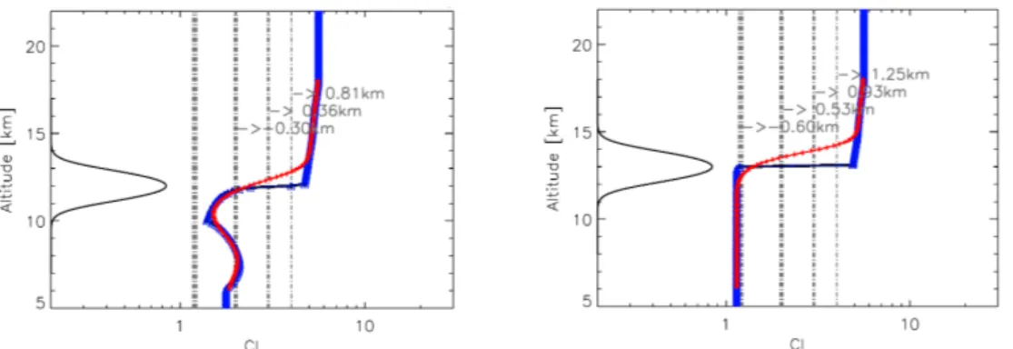
thick cloud is only filling the lower part of the FOV, the attributed CTH may overesti-mate the real CTH. This potential error source was investigated in detail by modelled cloud index profiles for various cloud conditions and background atmospheres (Fig. 3). We calculated radiance profiles of the analysed wavelength regions to compare the
5
cloud index for varying cloud altitude (6–20 km) and layer thickness (0.5 and 2 km), and extinction ε. Simulations were carried out with the line by line radiative transfer code RFM (Dudhia et al., 2002). Scattering processes were neglected. For a full set of simulations a realistic parameter space was chosen, i.e. CTHs between 6 and 16 km, different reference gas atmospheres, cloud extinctions from 10+1 to 10−4km−1 at a 10
wavelength of 12 µm, and box type cloud layers with vertical extension iof 0.5, 1, and 2 km. The calculations were performed on a 100 m vertical gird. The pencil beam ra-diance profiles were afterwards convolved with the FOV. By comparing the input CTH and the simulated CTH we estimate the maximum error in CTH for multiple CI thresh-olds (grey vertical lines in Fig. 3). Four different threshold values (1.2, 2, 3, 4) have 15
been investigated for the various cloud layer extinctions and cloud vertical thickness. A detection threshold of 4 and 4.5 was applied for the Michelson Michelson Interfer-ometer for Passive Atmospheric Sounding (MIPAS) instrument (Fischer et al., 2008) in various studies for the detection of the usually optically thin PSCs (e.g. Spang et al., 2003; Höpfner et al., 2005). Sembhi et al. (2012) showed that CIthresvalues up to 6 are
20
acceptable for the MIPAS measurements depending on the latitude and altitude region of interest.
Figure 3 shows the CI profiles of the pencil beam simulations and the CI pro-file with the FOV convolution for a homogeneous cloud layer for an optically thin (ε=3×10⁻³km−1) cloud between 10 to 12 km (CTH=12 km) and an optically thick 25
(ε=10−1km−1) cloud between 11–13 km (CTH=13 km). The conservative threshold
CIthres=1.2 detects only optically thick clouds and consequently the CTH is under-estimated due to the FOV effect. Optically thinner clouds are only detectable with
ACPD
14, 12323–12375, 2014Satellite observations of cirrus clouds in the Northern Hemisphere
R. Spang et al.
Title Page
Abstract Introduction
Conclusions References
Tables Figures
◭ ◮
◭ ◮
Back Close
Full Screen / Esc
Printer-friendly Version
Interactive Discussion
Discussion
P
a
per
|
D
iscussion
P
a
per
|
Discussion
P
a
per
|
Discuss
ion
P
a
per
|
shows a maximum possible CTH error (∆
max2) of 0.6 km for all simulations. Higher thresholds result in higher detection sensitivity but cause higher uncertainties in CTH (∆max 3=0.9 km for CIthres=3 and∆max 4=1.4 km for CIthres=4) for optical thick clouds
withε >10−1km−1. Optically thinner clouds usually cause smaller maximum CTH er-rors.
5
However, the optically thin and thick example in Fig. 3 show that higher detection sen-sitivity will cause an overestimation of the CTH, in the examples for 0.8 and 1.25 km for CIthres=4. In addition it should be noted that the actual CTH error of a measure-ment depends not only on CIthres, but also on the relative distance of the measured tangent heights to the actual “real” cloud top (sampling). For CRISTA measurements
10
the distances of the tangent point to the “real” CTH in the atmosphere are statistically almost equally distributed with a maximum distance of±1 km due to the 2 km vertical sampling. The∆
maxvalues above are errors of a worst case scenario and represent the upper extreme of the FOV effect. Half of all detections of optically thick clouds will have
a∆CTHsmaller than∆max/2, due to the fact that the FOV error for optical thick clouds 15
declines linearly with declining difference between the sampled observation height and
the “real” CTH (see Fig. 3).
In conclusion, the mean CTH error due to the FOV (for optical thick clouds) ∆FOV
is consistent with ∆max/2. For optically thinner clouds ∆max becomes systematically
smaller (e.g. compare Fig. 3a for thin and Fig. 3b for thick conditions) and for the more
20
stringent CIthres=2 these clouds are only detectable at an observations height below the actually “true” CTH (negative CTH errors in Fig. 3a). In the following analyses we used two thresholds, CIthres=2 and CI
thres=3, for optimisation and best trade-off between quantified FOV effects and best detection sensitivity for optically thin clouds.
The chosen CI values are equivalent to extinction coefficients ofε >∼5×10⁻³km−1and 25
ε >∼2×10⁻³km−1respectively, and correspond to∆FOV2=250 m and∆FOV3=450 m.
ACPD
14, 12323–12375, 2014Satellite observations of cirrus clouds in the Northern Hemisphere
R. Spang et al.
Title Page
Abstract Introduction
Conclusions References
Tables Figures
◭ ◮
◭ ◮
Back Close
Full Screen / Esc
Printer-friendly Version
Interactive Discussion
Discussion
P
a
per
|
D
iscussion
P
a
per
|
Discussion
P
a
per
|
Discuss
ion
P
a
per
|
is unknown and therefore difficult to quantify. The slanted ice water path (IWP), the
IWC integrated along the line of sight (Spang et al., 2012, and also Sect. 5.4), deter-mines the actual optically thickness of the measured spectrum in the limb direction. Radiative transport model calculations for a characteristic diversity of cirrus size dis-tribution parameter (Griessbach et al., 2014) under the assumption of vertically and
5
horizontally homogeneous cloud layers show that the largest FOV induced CTH er-rors∆
max(forε >10 −1
km−1) can be generated from a cloud layer with IWC>∼3 ppmv (>0.5 mg m−3) (Spang et al., 2007; Fig. 5). This is a common value in IWC in-situ mea-surements in the upper troposphere, typically close and or slightly greater than the typical median values (Krämer et al., 2009) in the corresponding temperature range of
10
the CRISTA measurements. Consequently, it is very likely that the CRISTA statistics also include a certain amount of underestimated CTHs by optically very thin clouds (IWC≪3 ppmv).
Uncertainties in CTH determination from broken cloud segments along the line of sight in combination with the horizontal integration of the limb information and from
15
the cross track extension of the FOV (30 arcmin,∼15 km) are not considered in the present analysis. However, both effects cause a reduction in detection sensitivity and
results in an underestimation of the CTH in respect to the true CTH. Consequently falsified detections above the local tropopause can be excluded by these two effects.
2.4 Radiosonde data
20
In this study we used the radiosonde station composite data from the University of Wyoming, Department of Atmospheric Science. For August 1997, a time period embed-ding the complete CRISTA-2 mission, around 5000 radiosonde launches were available for coincident comparison of tropopause location with respect to CTHs from CRISTA and for the global validation of an improved tropopause determination with the ERA
25
ACPD
14, 12323–12375, 2014Satellite observations of cirrus clouds in the Northern Hemisphere
R. Spang et al.
Title Page
Abstract Introduction
Conclusions References
Tables Figures
◭ ◮
◭ ◮
Back Close
Full Screen / Esc
Printer-friendly Version
Interactive Discussion
Discussion
P
a
per
|
D
iscussion
P
a
per
|
Discussion
P
a
per
|
Discuss
ion
P
a
per
|
clearly visible in the blue temperature profile. The horizontal lines are indicating the re-trieved CTH from CI and lapse rate tropopause based on coincident ERA Interim tem-peratures (details see Sect. 2.5). Usually radiosonde RH measurements around the tropopause have a low accuracy and act more like a qualitative measure of humidity. Nevertheless, RH and the ice saturation temperature profile indicate atmospheric
con-5
ditions around the tropopause that allow for the existence of ice. This is in coincidence with the slightly higher cloud layer detected by CRISTA, where CTH and tropopause height (TPH) are suggesting a cloud above the local tropopause.
2.5 Improved determination of the lapse rate tropopause for ERA Interim
Accurate tropopause height determination is crucial for the location of cloud events with
10
respect to the tropopause as PM2011 already showed for the CALIPSO cloud detec-tion. For our analyses we used the ERA Interim reanalysis data on hybrid coordinates (Dee et al., 2011) with original model resolution (60 levels and 600–1000 m resolution around the tropopause) for the computation of the tropopause height. A three step approach is applied to the data. (1) For each CRISTA tangent height the surrounding
15
four ERA temperature and geopotential height profiles are determined. Then the lapse rate tropopause was defined for each profile as the lowest pressure (altitude) level at which the lapse rate is 2 K km−1or less. The lapse rate should not exceed this thresh-old for the next higher levels within 2 km (WMO, 1957). The vertical resolution of the retrieved TPH cannot be better than the vertical grid resolution of the temperature data
20
and hence, can produce a significant positive bias for analyses with tropopause related altitude coordinates (PM2011). In step (2) we applied a vertical spline interpolation with 30 m vertical resolution to the temperature profile around the actual TPH of step 1 and repeated the TPH computation with the artificially higher vertical resolution. Finally, in step (3) the weighted mean with distance of the four surrounding grid points of the
ob-25
ACPD
14, 12323–12375, 2014Satellite observations of cirrus clouds in the Northern Hemisphere
R. Spang et al.
Title Page
Abstract Introduction
Conclusions References
Tables Figures
◭ ◮
◭ ◮
Back Close
Full Screen / Esc
Printer-friendly Version
Interactive Discussion
Discussion
P
a
per
|
D
iscussion
P
a
per
|
Discussion
P
a
per
|
Discuss
ion
P
a
per
|
was found, because the single TPH values are not attached to the altitude grid points of the analysis data anymore.
Comparisons with radiosonde data set for August 1997 show a good correspon-dence between the TPHhr and the lapse rate tropopause of the radiosonde for the coincidences with CRISTA profiles (see also Fig. 2). A statistical analysis of the diff er-5
ence in TPH between 5304 sonde profiles in the latitude range 30◦N and 80◦N and the ERA Interim based TPHhrfor August 1997 showed a mean difference of 0.015 km and
a standard deviation of 650 m. The latter value is exactly the same value as found in the analysis of PM2011 for a comparison between radiosonde and National Center of Environmental Prediction Global Forecast System (GFS) data for a June-July-August
10
season in 2007. The good correspondence gives us confidence that the described TPHhr is the best possible and reliable approach for a tropopause determination for each CRISTA profile. In addition, the standard deviation of the differences appears to
be a realistic estimate for the uncertainty of TPHhr.
3 CRISTA cloud top height occurrence with respect to the tropopause
15
3.1 Tropopause derived from radiosonde data
A comparison of tropopause heights determined from radiosonde measurements with the detected CTHs in the tropopause region allows a first quantitative assessment of the indication for frequent observation of optically thin clouds by CRISTA in the LMS like illustrated in Fig. 1. A miss time of 2 h and miss distance of 200 km coincidence
20
criteria were chosen to minimise uncertainties in the comparison. For 158 CTH detec-tions close to the tropopause and north of 40◦N (with CIthres=3, CTH-TPH>−500 m, and TPH defined from co-located ERA Interim temperatures) we found 188 coincident radiosonde profiles. The tropopause of 62 radiosonde profiles (∼33 %) is pinpointed more than 500 m below the coincident CTH of CRISTA. This indicates a remarkable
25
ACPD
14, 12323–12375, 2014Satellite observations of cirrus clouds in the Northern Hemisphere
R. Spang et al.
Title Page
Abstract Introduction
Conclusions References
Tables Figures
◭ ◮
◭ ◮
Back Close
Full Screen / Esc
Printer-friendly Version
Interactive Discussion
Discussion
P
a
per
|
D
iscussion
P
a
per
|
Discussion
P
a
per
|
Discuss
ion
P
a
per
|
altitude clouds in the LMS are a common feature or a rare incidence. However, the only limited number of good coincidences between CRISTA and radiosonde measurements with respect to adequate miss time and distance criteria allows no profound conclu-sions on this question. A statistical analysis of all cloud observed in the tropopause region together with the collocated tropopause heights based on ERA Interim may
5
solve this problem.
3.2 Statistical analysis with tropopause derived from ERA Interim
For the statistical analysis of cloud occurrences around the tropopause we choose a vertical coordinate independent of the temporal and spatial location of the tropopause. Therefore thermal tropopause relative coordinates are applied in the
fol-10
lowing similar to PM2011. These coordinates are used extensively in chemical tracer analyses (e.g. Tuck et al., 1997; Pan et al., 2007; Kunz et al., 2013) and temperature profile analyses (e.g. Birner et al., 2006). The actual distance of a detected CTH to the tropopause is defined by∆CTH=CTH
i−TPHi where the indexi is attributed to an indi-vidual measurement profile. For displaying results it is often more helpful to adjust the
15
reference altitude to the mean tropopause height (TPHmean). The tropopause related altitudeZr is then defined by:
Zr=Ztrop+(Z−Ztrop), (1)
withZ the observations altitude or the CTH,Ztropthe individual tropopause, and Ztrop
20
for example a daily or monthly zonal mean tropopause. Here we use forZtropthe zonal mean tropopause during the CRISTA-2 measurement period.
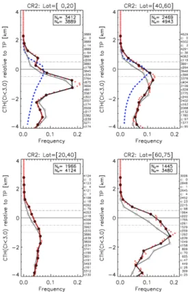
Figure 4 presents the results of CTH height occurrence frequencies (COF) in re-spect to the single profile tropopause location defined by the approach above and a vertical grid size of 0.5 km. Latitude bands covering the whole Northern Hemisphere
25
ACPD
14, 12323–12375, 2014Satellite observations of cirrus clouds in the Northern Hemisphere
R. Spang et al.
Title Page
Abstract Introduction
Conclusions References
Tables Figures
◭ ◮
◭ ◮
Back Close
Full Screen / Esc
Printer-friendly Version
Interactive Discussion
Discussion
P
a
per
|
D
iscussion
P
a
per
|
Discussion
P
a
per
|
Discuss
ion
P
a
per
|
different for the various latitude bands. A joint feature is the location of the maximum
in COF in a layer 0.75 to 1.25 km below the tropopause for almost all latitude bands. In parts this is caused by the limb geometry. The probability to detect a cloud along the line of sight located above the actual tangent height is enhanced with penetrating deeper into the troposphere. This effect causes artificially overestimated COFs below 5
the real maximum in the COF distribution and is especially a large bias in the tropics, where horizontally small extended and patchy distributed cloud systems (<50 km), e.g. by deep convection events, are generating unrealistic high COFs in limb observations (Kent et al., 1997; Spang et al., 2012). Note that CTHs assigned to such observations are actually low biased.
10
Only the subtropics show the COF maximum at slightly lower altitudes. But more re-markable, generally very low COF values are found around the tropopause compared to the three other latitude bands. This local minimum at 20–40◦ latitude in cloud prob-ability has been already observed in various limb sounder observations around the tropopause (e.g. Wang et al., 1996; Spang et al., 2002, 2012).
15
Figure 4 presents the COF values for both CI threshold values. The frequencies for CIthres=3 are systematically higher than for the less sensitive threshold CI
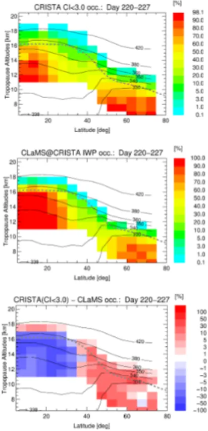
thres=2, and more clouds are detected well above the predefined tropopause and also above the maximum in the COF distribution. For the more sensitive detection method CIthres=3 a COF of 3 and 4 % (217 events in total) is found in the altitude grid box 500–1000 m
20
for mid- and high-latitudes respectively. Even in the 1000–1500 m grid box above the tropopause COFs of ∼1 % are observed in both latitude bands (59 events). These COF values above the tropopause indicate significantly larger occurrence rates than found in ground based lidar observations (e.g. Noel and Haeffelin, 2007; Rolf, 2013).
The typically observed frequencies of 4–10 % of cross tropopause cirrus were referred
25
ACPD
14, 12323–12375, 2014Satellite observations of cirrus clouds in the Northern Hemisphere
R. Spang et al.
Title Page
Abstract Introduction
Conclusions References
Tables Figures
◭ ◮
◭ ◮
Back Close
Full Screen / Esc
Printer-friendly Version
Interactive Discussion
Discussion
P
a
per
|
D
iscussion
P
a
per
|
Discussion
P
a
per
|
Discuss
ion
P
a
per
|
In addition, the tropics show a pronounced local maximum well above the tropopause. The 100 m running mean statistic of 500 m grid boxes (red symbols) indi-cates that the feature is not a sampling artefact caused by an interplay of the measure-ment altitudes with the vertical gridding of the COF analysis. This interesting feature will be studied in more detail in a future study.
5
3.3 Significance tests of cloud top occurrence distribution
We have investigated in detail how the measurement uncertainties of the tangent point altitude, tropopause height, and cloud top height (Sect. 2) might influence or even falsify the COF statistics. Where TPH and tangent altitude errors are well described by Gaussian distribution (with corresponding standard deviations), the CTH error (∆CTH) 10
caused by the vertical FOV effect for optically thick clouds acts like a positive bias in
the cloud top height determination.
Monte Carlo (MC) simulations with the CRISTA measurement ensemble of cloudy and non-cloudy profiles have been performed taking into account (a) statistical and (b) systematic error sources. For both types of simulations all CTHs above the tropopause
15
were excluded from the dataset and the remaining CTH observations have been mod-ified by a randomly distributed statistical uncertainty or a systematic positive offset
value with a Gaussian amplitude. The results show that a statistical (noise) errors like the TPH uncertainty withσTPH=650 m or even an overestimated value of 1000 m can-not reproduce the measured vertical COF distribution and cancan-not create the relative
20
large COFs observed above the tropopause.
For testing the systematic errors we applied to all CTH observations below the tropopause a FOV-like, Gaussian-shaped, and only positive offset distribution. This
approach is equivalent to the assumption that all clouds below the tropopause are optically thick (upper limit), are creating a positive offset, and are detected with the 25
ACPD
14, 12323–12375, 2014Satellite observations of cirrus clouds in the Northern Hemisphere
R. Spang et al.
Title Page
Abstract Introduction
Conclusions References
Tables Figures
◭ ◮
◭ ◮
Back Close
Full Screen / Esc
Printer-friendly Version
Interactive Discussion
Discussion
P
a
per
|
D
iscussion
P
a
per
|
Discussion
P
a
per
|
Discuss
ion
P
a
per
|
to the original statistic. Larger|σFOV| produces overestimated COF values well above the tropopause (>1.5 km), significant underestimates below the tropopause, and can be excluded. Surprisingly, the MC simulations were not able to reproduce the tropical COF distribution with the positive bias approach. These two negative tests, large|σFOV| and irreproducible tropical COF distribution, are additional constraints for a systematic
5
and large FOV effect above the tropopause. In addition it is very unlikely that all clouds
around the tropopause are optically thick (only<50 %, see Sect. 2.3). Consequently it is very unlikely that this type of clouds is responsible for an artificial enhancement in COF above the tropopause like observed by CRISTA in Fig. 4.
An additional and substantial argument against a large systematic FOV effect is the 10
different behaviour between tropical and mid/high latitudes in the measurements
com-pared to the simulations. A positive bias for optical thick clouds should modify the pro-nounced maximum peak 1 km below tropical tropopause in the following way and is confirmed in the MC simulations: the observations would show a broader distribution and a significant extent of enhanced COF values in direction to higher altitudes similar
15
to the mid and high latitudes. But this behaviour is not observed in the tropical measure-ments (Fig. 4a). A shift to higher altitudes can be reproduced in the error simulations with |σFOV|=750 m, but contrariwise it is creating strong enhanced COFs just below tropopause and reduced values below. The overall effect in the simulations, a positive
shift of the whole distribution, is not observed in the original data.
20
In conclusion, taken all uncertainties into account the CRISTA COF distribution indi-cates a significant amount of cirrus cloud observations in the lowermost stratosphere. To our knowledge this is the first time such findings are reported for space-borne limb measurements.
3.4 Comparison with CALIPSO
25
ACPD
14, 12323–12375, 2014Satellite observations of cirrus clouds in the Northern Hemisphere
R. Spang et al.
Title Page
Abstract Introduction
Conclusions References
Tables Figures
◭ ◮
◭ ◮
Back Close
Full Screen / Esc
Printer-friendly Version
Interactive Discussion
Discussion
P
a
per
|
D
iscussion
P
a
per
|
Discussion
P
a
per
|
Discuss
ion
P
a
per
|
period and observations geometry are very different (7 day mean vs. multi annual
sea-sonal mean and limb vs. nadir). In this region even the absolute COF values are in close agreement. However, in the grid boxes 500–1000 m and 1000–1500 m above the tropopause CRISTA detected∼2 times more clouds than the CALIPSO climatology. Below the tropopause the limb sounder statistic shows a substantial larger maximum
5
in COF. This is primarily due to the long limb path integration and the artificially en-hanced number of cloud detections well below the tropopause by higher altitude cloud fragments along the line of sight, and only secondary due to the better detection sen-sitivity for horizontally extended clouds in the limb compared to the short nadir viewing direction.
10
The tropical distribution looks more different, especially below the tropopause, where
again the overestimation due the limb geometry plays a role. At the tropopause (±500 m), where this effect is negligible, both instruments show similar COFs. Well
above the tropopause (500 to 1500 m) CRISTA COFs are again significantly larger than CALIPSO and indicate the presence of optically very thin clouds, which are
cur-15
rently not detected in the CALIPSO data products (see also Sect. 1). It should be noted that the CALIOP instrument may have observed these clouds, but the current detec-tion threshold of the operadetec-tional data products is not capable to detect ultra thin cirrus clouds. This was already shown by Davis et al. (2011) in a validation study with airborne lidar and in situ particle measurements. Modified detection schemes with larger
hori-20
zontal averaging of the high resolution Level 1 profile data of CALIOP (e.g. 30 or 50 km instead of currently 5 km) will substantially improve the detection sensitivity for ultra thin cirrus clouds (M. Vaughan, personal communication, 2014). The current detection limit for cirrus clouds averaged horizontally to 5 km for the 532 nm extinction channel is in the range of 0.005 and 0.02 km−1, which represents an equivalent IWC of 0.1 to
25
ACPD
14, 12323–12375, 2014Satellite observations of cirrus clouds in the Northern Hemisphere
R. Spang et al.
Title Page
Abstract Introduction
Conclusions References
Tables Figures
◭ ◮
◭ ◮
Back Close
Full Screen / Esc
Printer-friendly Version
Interactive Discussion
Discussion
P
a
per
|
D
iscussion
P
a
per
|
Discussion
P
a
per
|
Discuss
ion
P
a
per
|
4 Horizontal distribution of water vapour and clouds in the UTLS
4.1 Cloud top height distributions
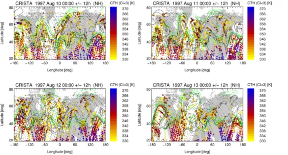
Four days during CRISTA-2 have a measurement net dense enough for hemispheric analyses of horizontal structures in cloud and trace gas distributions. Figure 5 presents the daily cloud top height distribution detected with the algorithms described in
5
Sect. 2.2 for 10 to 13 August at midnight±12 h. Potential temperature (Θ) has been
used as vertical coordinate and CTHs in km are converted to Θ by coincident ERA
Interim temperature and geopotential height information. Only clouds detected in the altitude range 330 to 370 K are presented, an atmospheric layer usually located in the lower half of the lowermost stratosphere (LMS) at mid and high latitudes, and clearly in
10
the upper troposphere and tropopause region for the tropics and subtropics. The observations show frequent high cloud top Θ (Θ
CTH) events in regions where elongated PV contours as well as horizontal winds (green contours) are suggesting strong horizontal transport and mixing processes extending from mid latitudes (∼40◦N) to high northern latitudes. Main regions are over the eastern pacific with extension in
di-15
rection to Alaska, the north-eastern US directed to Greenland, from North-Atlantic and Central-Europe towards northern Scandinavia and the Baltic region, and from China towards Siberia. High altitude clouds are observed up to the northern edge of the CRISTA measurements at 74◦N (e.g. over northern Scandinavia and the Baltic Sea on 10 August). During the four days of observations the frequency for highΘCTH(>350 K) 20
events north of the subtropical jet region seems to decline.
The highest detected ΘCTH (350–360 K) are in most cases above the local
tropopause indicating an origin of the detected cloudy air masses in the LMS. CTHs below 350 K in regions dominated by high CTHs (e.g. in the Scandinavia-Baltic-Sea streamer) may be caused by a “real” lower altitude tropospheric cloud, but can also
25
ACPD
14, 12323–12375, 2014Satellite observations of cirrus clouds in the Northern Hemisphere
R. Spang et al.
Title Page
Abstract Introduction
Conclusions References
Tables Figures
◭ ◮
◭ ◮
Back Close
Full Screen / Esc
Printer-friendly Version
Interactive Discussion
Discussion
P
a
per
|
D
iscussion
P
a
per
|
Discussion
P
a
per
|
Discuss
ion
P
a
per
|
significant differences in the absolute tangent height between even subsequent orbits
(up to 1 km) with close geographical co-location. Consequently a large cloud struc-ture with nearly constant CTH may be detected at different altitudes in two subsequent
orbits at higher latitudes or in the tropics on up and down leg of a single orbit.
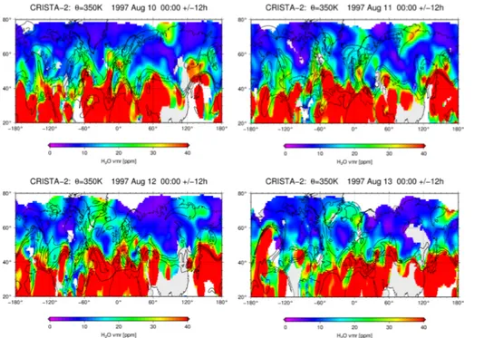
4.2 Water vapour measurements during CRISTA-2
5
The horizontal distribution of the CRISTA water vapour at the 350 K isentrope is illus-trated in Fig. 6 for the same days like in Fig. 5. For better visualisation the data of individual CRISTA H2O profiles have been first interpolated to a constant theta level (here 350 K). Vertical interpolation around the tropopause and below take always the risk that it create some numerical diffusion and artificially enhanced water vapour mix-10
ing ratios at the grid level due to the strong exponential gradient in the mixing ratio profile below the tropopause. This effect was minimized by logarithmic interpolation.
In a second step a horizontal interpolation on a regular grid (1◦×1◦) was performed by means of distance-weighted averaging. Data gaps in the tropics are mostly due to clouds.
15
The CRISTA water vapour measurements were validated with the Microwave Limb Sounder (MLS) and airborne in situ instruments (Offermann et al., 2002). The
compar-isons showed good agreement in the coincidence statistics and a retrieval accuracy of 10 % was estimated for the data. The precision of the data is 8 % for values>10 ppmv, and 8–15 % for smaller values (Schaeler et al., 2005). Consequently, the horizontal
20
structures in Fig. 6 are reliable.
Transport of water vapour from the tropical troposphere into the LMS on the 350 K isentropic surface seems evidential in Fig. 6. Shown are water vapour values as ob-served by CRISTA-2 on 10 to 13 August at midnight ±12 h. Rossby wave breaking events result in an erosion of the tropopause that can by identified by the cut-offof PV 25
ACPD
14, 12323–12375, 2014Satellite observations of cirrus clouds in the Northern Hemisphere
R. Spang et al.
Title Page
Abstract Introduction
Conclusions References
Tables Figures
◭ ◮
◭ ◮
Back Close
Full Screen / Esc
Printer-friendly Version
Interactive Discussion
Discussion
P
a
per
|
D
iscussion
P
a
per
|
Discussion
P
a
per
|
Discuss
ion
P
a
per
|
of water vapour deep into the LMS. These horizontal structures of high water vapour are nearly coinciding with the “unusual” high CTH observation shown in Fig. 5.
The water vapour values do not include the locations of optically thicker cloud obser-vations, because a corresponding filter (CI<2) was applied before the retrieval. How-ever, it is evident that cloudy areas are embedded in regions of relatively high water
5
vapour values. More quantitative analyses exclusively from the satellite observations are difficult, because for most cloudy CRISTA observations no adequate water retrieval
is available.
5 Comparison with the CLaMS model
5.1 The CLaMS model
10
The Chemical Lagrangian Model of the Stratosphere (McKenna et al., 2002a, b; Konopka et al., 2007) is a chemistry transport model based on three-dimensional for-ward trajectories, describing the motion of air parcels. Additional to advection by winds, irreversible small-scale mixing between air parcels induced by deformation of the large scale flow is considered in the model (McKenna et al., 2002a; Konopka et al., 2004).
15
The mixing intensity is controlled by the local Lyapunov coefficient of the flow, thus
lead-ing to stronger mixlead-ing in regions of large flow deformations. The sensitivity of simulated UTLS water vapour on the intensity of this quantity is discussed by Riese et al. (2012). The model uses a hybrid of pressure and potential temperature as vertical coordinate system first proposed by Mahowald et al. (2002).
20
5.2 Model setup
The CLaMS simulation was started in mid May 1997, three months in advance of the CRISTA observations, to give the model enough time for spin-up. The model was driven by six hourly ERA Interim re-analyses with a mixing time step of 24 h. The calculation of water vapour in CLaMS includes a simplified dehydration scheme, similar to that
ACPD
14, 12323–12375, 2014Satellite observations of cirrus clouds in the Northern Hemisphere
R. Spang et al.
Title Page
Abstract Introduction
Conclusions References
Tables Figures
◭ ◮
◭ ◮
Back Close
Full Screen / Esc
Printer-friendly Version
Interactive Discussion
Discussion
P
a
per
|
D
iscussion
P
a
per
|
Discussion
P
a
per
|
Discuss
ion
P
a
per
|
applied in von Hobe et al. (2011). Gas phase water in CLaMS is initialized at the be-ginning of the simulation utilizing the specific humidity taken from ERA Interim data. Boundaries are updated every CLaMS step from ERA Interim data as well. The lower boundary for this run is at 250 K with respect to the hybrid vertical coordinate, corre-sponding to approximately 500 hPa.
5
The formation of ice is parameterised either by using a fixed value of 100 % for saturation over ice (a value commonly used) or by a temperature dependent param-eterisation for heterogeneous freezing (Krämer et al., 2009). The latter method was finally used in the model simulations presented below. This parameterisation results in saturation values between 120 and 140 % for the temperature range from 180 to 230 K.
10
Water vapour with values above these saturation levels is removed from gas phase and added to the ice water content. Water vapour and ice water content are transported and mixed like any other tracer or chemical species. Evaporation at 100 % saturation and sedimentation of ice by assuming a uniform particle density and size distribution (Krämer et al., 2009) as well as parameterised processes like re- and de-hydration
15
are considered, with the only exception of re-hydration by formerly sedimented parti-cles. For sedimentation the terminal settling velocity is calculated. The corresponding sedimentation length is compared with a characteristic height defined by the vertical resolution of the model around the tropopause (∼650 m for this simulation), and the related fraction of ice is removed. This mechanism was successfully used for long term
20
studies with CLaMS (Ploeger et al., 2011, 2013). The horizontal resolution of the sim-ulations is in the range of 70 km.
5.3 IWC and water vapour distribution in the model
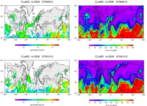
In a first step we investigated CLaMS model results for water vapour and ice water content on synoptic maps of isentropic surfaces like in Fig. 7. Afterwards model output
25
ACPD
14, 12323–12375, 2014Satellite observations of cirrus clouds in the Northern Hemisphere
R. Spang et al.
Title Page
Abstract Introduction
Conclusions References
Tables Figures
◭ ◮
◭ ◮
Back Close
Full Screen / Esc
Printer-friendly Version
Interactive Discussion
Discussion
P
a
per
|
D
iscussion
P
a
per
|
Discussion
P
a
per
|
Discuss
ion
P
a
per
|
In the examples of Fig. 7 isentropic surfaces ofΘ =350 K are selected, which
rep-resent a nearly constant geometrical height with changing latitude, where isentropical transport can cross from the tropical UT into the mid latitude LS. In Fig. 7 both IWC and water vapour show distinctive streamer structures on two successive days (9 and 10 August). The streamers are elongated and spread out to mid and high northern
5
latitudes. Especially the water vapour distribution suggests that regions of high wa-ter vapour are peeled offfrom the subtropical jet region, as typically observed in PV
fields during Rossby wave breaking events (e.g. Homeyer and Bowman, 2013). These sub-tropical air masses are transported to and mixed in at high latitudes, where under favourable conditions the formation of cirrus clouds might be possible. Fine structures
10
of water vapour and IWC can be observed similar to and more fine structured than the superimposed PV contours. The IWC structures are less pronounced and indicate significant less cloud formation at mid and high latitudes in contrast to the CRISTA observations (Fig. 5).
5.4 How to compare global model data and limb measurements?
15
For a quantitative comparison between the model data and limb measurements it is crucial to take into account the observation geometry and to apply averaging kernels of the instrument to the model data. In an optimised but very expensive process cur-rent investigations simulate the original measurement quantity of the instrument (e.g. here IR radiances) by a specific instrument simulator based on 3-D input parameter of
20
a climate chemistry model (e.g. Bodas-Sacedo et al., 2011). This approach will reduce the uncertainties usually introduced by the complex retrieval process of the instrument target parameter (e.g. IWC, specific humidity or other trace gases) and is used for the validation of climate models. The detailed consideration of the observation geometry is especially important for comparisons with cloud measurements in the limb (e.g. Spang
25
ACPD
14, 12323–12375, 2014Satellite observations of cirrus clouds in the Northern Hemisphere
R. Spang et al.
Title Page
Abstract Introduction
Conclusions References
Tables Figures
◭ ◮
◭ ◮
Back Close
Full Screen / Esc
Printer-friendly Version
Interactive Discussion
Discussion
P
a
per
|
D
iscussion
P
a
per
|
Discussion
P
a
per
|
Discuss
ion
P
a
per
|
In the first step, the temporal offsets between the asynoptic measurement times of
the satellite and the synoptic time steps in the model output (every 24 h) have been compensated. For this purpose backward trajectories of all CRISTA observations below 25 km to the next synoptic model output time, usually every 24 h at 12:00 UTC were computed. Starting from these synoptic locations the cirrus module of CLaMS was
5
run forward in time to the asynoptic time of the individual CRISTA observation. By this approach the formation and evaporation of ice clouds in a time frame of maximum 24 h between model output (12:00 UTC) and observation is taken into account.
Secondly, we implemented an integration of the signal along the line of sight. A limb ray tracing from the original position of the CRISTA satellite to the tangent point and
10
the follow-on to deep space has been applied to sample the model data. In case of CRISTA the tangent height layer for the 1.5 km FOV has an extension of ∼280 km. Deeper tropospheric observations result in a factor of 2–3 longer (e.g. in the tropics) effective path lengths through the atmosphere where a cloud can occur. In the tropics
for a tangent height at 10 km the maximum potential cloud occurrence altitude extents
15
up to a height of∼18 km and a corresponding line of sight segment of∼640 km should be considered in the limb ray tracing.
Spang et al. (2012) showed that limb IR measurements of cirrus clouds are most sensitive to the integrated surface area density along the limb path (area density path, ADP) and that ADP is a useful quantity for comparisons with global models, where the
20
limb path can be traced through the model output to generate the ADP quantity. The ADP and CI show an excellent correlation and ADP can be retrieved from the measured CI values (Spang et al., 2012). For a homogeneous limb path segment ADP and limb ice water path (IWP) are related by the simple equation:
ADP=3·IWP/(R
eff·ρice) (2)
25
ACPD
14, 12323–12375, 2014Satellite observations of cirrus clouds in the Northern Hemisphere
R. Spang et al.
Title Page
Abstract Introduction
Conclusions References
Tables Figures
◭ ◮
◭ ◮
Back Close
Full Screen / Esc
Printer-friendly Version
Interactive Discussion
Discussion
P
a
per
|
D
iscussion
P
a
per
|
Discussion
P
a
per
|
Discuss
ion
P
a
per
|
depending which parameters are known from the model or measurements:
IWP=
∞ Z
0
IWCdx=
∞ Z
0
V ·ρicedx= 1 3
∞ Z
0
A·Reff·ρicedx, (3)
whereReff and IWC are defined by the model,V andArepresent volume and surface area density respectively (Spang et al., 2012).
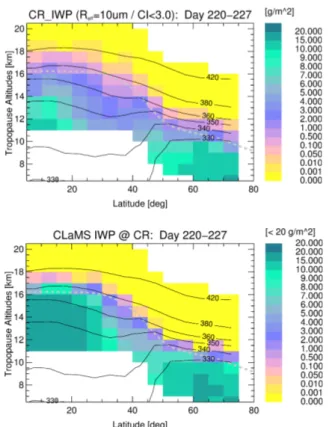
5
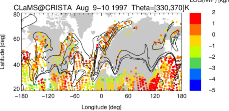
Finally we have used the simulated IWC to compute the IWP for a CRISTA-like cloud detection in the CLaMS model fields. A 30 km step width along the line of sight over a distance of±1000 km with respect to the tangent point has been chosen, which is in line with the horizontal resolution of the model. Then IWCCLAMShas been interpolated on the line of sight grid locations. A CTH detection is defined when the first (top) line
10
of sight beam of a CRISTA profile shows an IWPCLaMS>0. The latter fact is neglecting any detection sensitivity threshold of the instrument and represents therefore an upper limit of what a CRISTA-like instrument would detect in the cloudy atmosphere modelled by CLaMS.
An example of the CRISTA-like limb IWP is given in Fig. 8. All tangent heights
be-15
tween the 330 and 370 K isentrope with IWP>0 are presented for 1997 10 August 00:00 UTC±12 h. The results can be compared with Figs. 1 and 5a, even though these figures show the CTH of a measured profile. For a perfect agreement between model and measurement the CLaMS cloud detections should be exactly at the location where CRISTA observed a cloud. Obviously the model field of IWP shows a good agreement
20
with the cloud occurrence observed by CRISTA. Similar regions show the occurrence of clouds at mid and high latitudes. Some regions are extended larger in the observations than in the model (e.g. the east end of the North Atlantic to Baltic Sea streamer, the ex-tension over Alaska or over Kamchatka). However there are also a few regions where the model shows clouds but the observation is cloud free. But care should be taken in
25