1
Ashalata Panigrahi and
2Manas Ranjan Patra
Department of Computer Science, Berhampur University, Berhampur, India
ABSTRACT
With the increase in Internet users the number of malicious users are also growing day-by-day posing a serious problem in distinguishing between normal and abnormal behavior of users in the network. This has led to the research area of intrusion detection which essentially analyzes the network traffic and tries to determine normal and abnormal patterns of behavior.In this paper, we have analyzed the standard NSL-KDD intrusion dataset using some neural network based techniques for predicting possible intrusions. Four most effective classification methods, namely, Radial Basis Function Network, Self-Organizing Map, Sequential Minimal Optimization, and Projective Adaptive Resonance Theory have been applied. In order to enhance the performance of the classifiers, three entropy based feature selection methods have been applied as preprocessing of data. Performances of different combinations of classifiers and attribute reduction methods have also been compared.
KEYWORDS:
Intrusion detection, Artificial Neural Network, attribute reduction
1. INTRODUCTION
Information security is a serious issue while using computer networks. There has been growing number of network attacks which has challenged application developers to create confidence among the users. Researchers have looked at the security concerns from different perspectives. Intrusion Detection System is one such attempt which tries to analyze network traffic in order to detect possible intrusive activities in a computer network. There are two types of intrusion detection systems: misuse detection system and anomaly detection system.While the former is capable of detecting attacks with known patterns/signatures, the latter is augmented with the ability to identify intrusive activities that deviate from normal behavior in a monitored system, thus can detect unknown attacks. A range of techniques have been applied to analyze intrusion data and build systems that have higher detection rate.
improvement in attack detection and considerable drop in false alarm rate. Sung and S.Mukkamala [4] have proposed an approach for IDS with the use of Rank based feature selection and have shown that Support Vector Machines (SVMs) perform much better than Artificial Neural Networks (ANNs) in terms of speed of training, scale and accuracy. Lin NI, Hong Ying Zheng [5] have attempted to build an intrusion detection system using unsupervised clustering and Chaos Simulated Annealing Algorithm. Rung-Ching Chen et al. [6] have proposed a hybrid approach by combining Rough Set Theory(RST) for feature reduction and Support Vector Machine(SVM) for classification. Amir Azimi Alastic et al [7] formalized SOM to classify IDS alerts to reduce false positives. Alert filtering and cluster merging algorithms were used to improve the accuracy of the system; SOM was used to find correlation between alerts.
2.PROPOSED ANN BASED HYBRID CLASSIFICATION MODEL
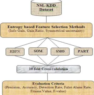
In this section we present our proposed model for classifying intrusion data in order to build an efficient intrusion detection system which can exhibit low false alarm rate and high detection rate. The model consists of two major layers as depicted in figure1.In the first layer irrelevant and redundant features are removed using three entropy based feature selection methods viz., Information Gain, Gain Ratio, Symmetrical Uncertainty. In the next layer the reduced data set is classified using four artificial neural network based techniques viz., Radial Basis Function Network(RBFN), Self-Organizing Map (SOM), Sequential Minimal Optimization(SMO), Projective Adaptive Resonance Theory (PART). Further, we have used the 10-fold cross validation technique for training and testing of the model. We evaluate the performance of the model using certain standard criteria.
17
3. METHODOLOGY
3.1. Radial Basis Function Network (RBFN )
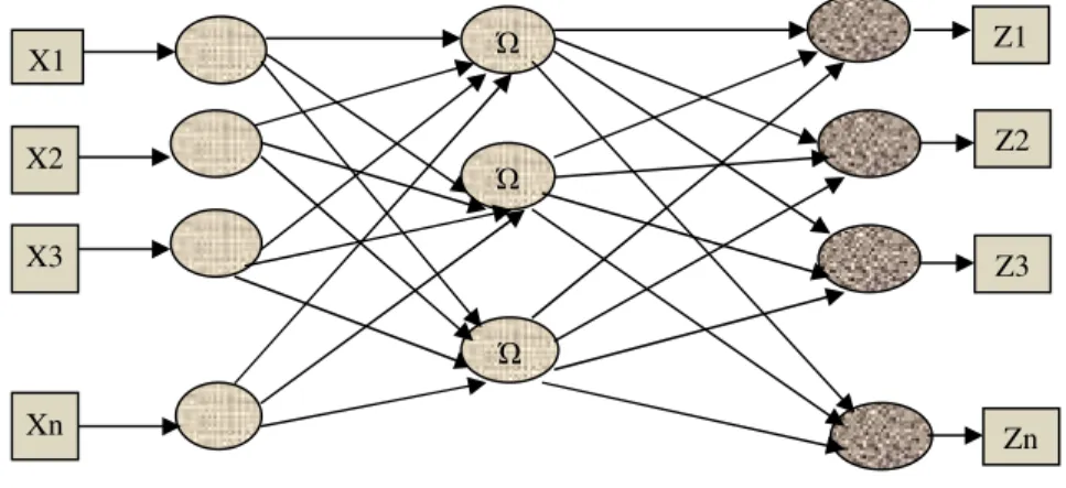
Radial Basis function (RBF) network is a nonlinear hybrid network which contains an input layer, a single hidden layer and an output layer [8]. The input layer accepts n number of inputs; the hidden layer consists of m radial basis functions and the output layer produces the response with the help of a linear additive function. The input neurons are linear, i.e., they pass the input to the hidden neurons without any processing. Using radial basis function the hidden neuron computes the signal and passes on these signals through weighted paths to the linear output neuron which sums them up and generates an output signal.
The neurons of the hidden layer are associated with a linear threshold activation function which produces the network output as:
yi = = ∑ wijФj (x) ………..……… (1)
where wij represents the weight of the connection between the hidden neuron j and the output neuron I and Фj (x) is the radial basis function applied at neuron j. We have used the following Gaussian function:
Ф(x) =exp( ( – ) )) › 0, x, c Є R ……….. (2)
The success of this model depends on determining the most suitable value for the parameter c [9]. The process begins by training an unsupervised layer which tries to find the Gaussian centers and the widths from the input data. During the unsupervised learning, the width of the Gaussians is computed based on the centers of their neighbors. The output of this layer is computed from the input data weighted by a Gaussian mixture.
3.2 Self Organizing Map (SOM)
The Self-Organizing Map (SOM) is a competitive network where the main objective is to transform an input data set of arbitrary dimension to one- or two-dimensional topological map [10]. SOM is motivated by the way information is processed in the cerebral cortex in human brain. The model was first proposed by the Finnish Professor Teuvo Kohonenand, thus referred to
Figure 2 Structure of RBF Network Ώ
Ώ Ώ
X1
X2
X3
Xn
Z1
Z2
Z3
as Kohonen map. SOM is an efficient technique to discover the underlying structure, e.g. feature map of the input data set by building a topology preserving map that describes neighborhood relations of the points in the data set [10]. SOM transforms a high dimensional input data domain to a low dimensional array of nodes. The SOM array is essentially a fixed size grid of nodes. Here, the training uses a competitive learning method wherein the neuron having a weight vector that is close to the input vector is adjusted towards the input vector. Such a neuron is referred to as the “winning neuron” or the Best Matching Unit (BMU). Next, the weights of the neurons close to the winning neuron are also adjusted. However, the magnitude of the change in each case depends on the distance from the winning neuron [11].
Let the real vectors X = {x1, x2, x3,………..xr } represent the input data, and a parametric real set of vectors Mi = { mi1, mi2,……….mik} be associated with each element i of the SOM grid where both X and Mi Є Rn . A decoder function, d( X, Mi ) defined on the basis of distance between the input vector and the parametric vector is used to define the image of the input vector onto the grid. One can use either the Manhattan or the Euclidean distance metric as the decoder function. The BMU is denoted as the index c of the node with a minimum distance from the input vector:
c = arg min { d(X, Mi) }………. (3)
SOM demands that Mi be shifted towards the order of X such that a set of values { Mi } is obtained as the limit of convergence of the equation:
mi ( t + 1 ) = mi (t) + α (t)* [x(t) − mi (t) ]* Hic ………. (4)
where Hic is a neighborhood function which models the interconnections between the nodes and is usually a Gaussian function which decreases with distance from the winner node c. The α (t) is the learning rate of the system.
3.3 Sequential Minimal Optimization(SMO)
The SMO algorithm is a specialized optimization approach for the SVM quadratic program. It combines the sparse nature of the support vector problem and the simple nature of the constraints in the Support Vector Machine Quadratic Programming (SVMQP) to reduce each optimization step to its minimum form[12]. SMO decomposes a large quadratic programming problem into a series of smaller quadratic programming problems. These small QP problems are solved analytically. The amount of memory required for SMO is linear in the training set size, which gives the ability to handle very large training sets.
Selecting α parameters
The SMO algorithm selects two values for the α parameters, viz., αi and αj, and optimizes the objective value for both αi and αj. In case of large data sets the values of αi and αj are critical as there can be m(m − 1) possible choices for αi and αj. Thus, the efficiency of SMO algorithm depends on the heuristics for determining αi and αj to maximize the objective function.
Optimizing αi and αj
19 • If y(i) ≠ y(j) , L = max(0, αi− αj ), H = min(C, C + αi− αj) ………… (5)
• If y(i) = y(j) , L = max(0, αi+ αj − C), H = min(C, αi+αj) ………. (6)
We intend to find αj so as to maximize the objective function. The optimal αj is given by
αj = αj – (y(j) (Ei – Ej)) / η ……….. (7)
where Ek = f( x(k) – y(k)) and η = 2‹x(i), y(j)› − ‹x(i), y(i)›− ‹x(j), y(j)›
Ek is the error between the SVM output on the k-th example and the true label y (k)
.
We clip αj to lie within the range [L, H] is
αj = {H, if αj>H
{αj, if L ≤ αj ≤ H ………(8)
{L, if αj< L
The value of αi can be calculated using the formula
αi = αi+ y(i) y(j) (αj(old) − αj) ………(9)
where αj(old) is the value of αj before optimization.
Computation of b Threshold
We select the threshold b such that the Karush-Kuhn-Tucker (KKT) [12] conditions are satisfied for the i-th and j-th examples. The threshold b1 is valid if 0 < αi< C and is given by
b1 = b – Ei – y(i) (αi − αi(old)) ‹x(i), x(i)› – y(j) (αj − αj(old) ) ‹x(i), x(j)› …………..(10)
b2 is valid if 0 <αj <C and is given by
b2 = b – Ej – y(i) (αi − αi(old)) ‹x(i), x(j)› – y(j) (αj − αj(old) ) ‹ x(j), x(j)› ………….(11)
If 0<αi< C and 0 < αj <C then both the thresholds are valid, and they will be equal.
b = { b1 if 0 < αi< C
{b2 if 0 < αj < C ………..(12) {(b1 + b2) / 2 otherwise
SMO Algorithm
Input:
C : Regularization Parameter Tol : Numerical tolerance
Max_Passes: Maximum number of times to iterate over α’s without changing the training data (x(1), y(1)), (x(2), y(2)), …….. (x(m), y(m))
Output:
Α Є Rm : Lagrange multipliers for solution b Є R: Threshold for solution
Initialize αi = 0, for all i, b=0 Initialize passes = 0
while(passes <max_passes) Num_changed_alphas = 0
fori = 1, 2,…..m
Calculate Ei = f((x(i), y(i)))
if ((y(i)Ei<tol&& αi< C (y(i)Ei>tol&& αi> 0)) Select j ≠ i randomly,
Calculate Ej = f((x(j), y(j)))
Save old α’s: αi(old) = αi , αj(old) = αj Compute L and H by (Eq. 1) and (Eq. 2)
if( L== H) continue to next i. Compute η by (5).
if( η>= 0)
continue to next i.
Compute new values for αj using (Eq. 3) and (Eq. 6)
if( αj − αj(old)< 10-5 ) Continue to next i.
Determine value for αi using (Eq. 7).
Compute b1, and b2 using (Eq. 8) and (Eq. 9) respectively. Compute b by (Eq. 10).
Num_changed_alphas : = Num_changed_alphas + 1.
end if end for
if (Num_changed_alphas == 0) passes := passes + 1
else passes := 0
21
3.4 Projective Adaptive Resonance Theory (PART)
Projective Adaptive Resonance Theory (PART) is an innovative neural network architecture proposed to provide a solution to high-dimensional clustering problems [13]. The architecture of PART is based on adaptive resonance theory (ART) neural network which is very effective in self-organized clustering in full dimensional space. ART focuses on the similarity of patterns in the full dimensional space and may fail to find patterns in subspaces of higher dimensional space. It is practically infeasible to find clusters in subspace clustering in all possible subspaces and then compare the results thus obtained due to the large number of possible subspaces of the order of 2m – 1 for large values of m. PART solves this problem by introducing a selective output signaling mechanism to ART.
The basic architecture of PART is similar to that of ART which is very effective in self-organized clustering in full dimensional spaces[14][15]. The PART architecture consists of a comparison layer F1 and a competitive layer F2. The F2 layer of PART follows the winner-take-all paradigm. The F1 layer selectively sends signals to nodes in F2 layer. A node in F1 layer can be active relative to only few nodes in F2 layer which is determined by a similarity test between the corresponding top-down weight and the signal generated in the F1 node. This similarity test plays an important role in the subspace clustering of PART.
Figure 3 PART Architecture
parameters control the degree of similarity of patterns which in turn controls the size of dimensions of the projected subspaces and the degree of similarity in an associated dimension.
The PART algorithm [13] is based on the assumptions that the model equations of PART have regular computational performance described by the following dynamic behavior during each learning trial when a constant input is imposed:
i. Winner-take-all paradigm: In this scenario, a node in the F2 layer that has the largest bottom-up filter input becomes the winner. After some finite time only this winner node is activated.
ii. Selective output signals remain to be constant. iii. Synaptic weights are updated using specific formulae.
iv. Dimensions of a specific projected cluster remainsnon-increasing in time.
PART Algorithm
Initialization
Number of nodes in F1 layeras the number of dimensions of the input data.
Choose the number n of nodes in F2 layer much larger than the expected number of clusters.
m: number of dimensions of the data space.
Set the internal parameter I, α, ζ and maximum iteration times M. I = (I1, I2,……….,Im ) is an input pattern.
α : The learning rate ζ = Small threshold
Choose the external input parameters ρ and σ ρ : Vigilance parameter
σ : Distance vigilance parameter
Step 1: Set all F2 nodes as being non-committed.
Step 2: For each data point in input data set, do Steps 2.1-2.6. 2.1 Compute hij for all F1 nodes ui and committed F2 nodes uj.
If all F2 nodes are non-committed, go to Step 2.3. 2.2. Compute Tj for all committed F2 nodes uj.
2.3 Select the winning F2 node uj. If no such F2 node is found then add the data
point to outlier and continue with Step 2.
2.4. If the winner is a committed node then compute rj else go to Step 2.6. 2.5. If rj≥ρ, go to Step 2.6, otherwise reset the winner uj and go back to Step 2.3.
2.6. Set the winner uj as the committed, and update the bottom-up and top-down
weights for winner node uj.
Step 3:Repeat Step 2 M times.
Step 4: For each cluster Cj in layer F2, compute the associated dimension set Dj. F2 layer becomes stable after a few iterations. M is usually a small number
4.EXPERIMENTAL SETUP
23
4.1 NSL-KDD Dataset
NSL- KDD is a dataset proposed by Tavallace et al. [16] that consists of intrusion data which is being used by researchers for experimentation. NSL-KDD data set is a subset of the original KDD99 dataset having the same features. The NSL-KDDdataset consists of all the 41 attributes and class label of KDD 99 data set. The class label contains four types of attacks, namely Denial of Service (DOS), User to Root (U2R), Remote to Local (R2L), Probe, and normal. This dataset has a binary class attribute. Also, it has a reasonable number of training and test instances which makes it practical to run the experiments.
The NSL-KDD has the following differences over the original KDD 99 dataset.
• It does not include redundant records in the training set, so that the classifiers will not be biased towards more frequent records.
• The number of selected records from each “difficulty level” is inversely proportional to the
percentage of records in the original KDD-99 dataset.
• It is possible to experiment on the entire NSL-KDD data set, thus avoids the need for random selection. Consequently, the evaluation results of different researchers will be consistent and comparable.
Table 1. Distribution of Records
Figure 4. Distribution of Classes
Each attack type comes under one of the following four main categories: DOS, U2R, R2L, Probes.
Class Number of Records
Percentage of Class Occurrences Normal 67343 53.48%
DOS 45927 36.45%
U2R 52 0.04%
R2L 995 0.78%
i) Denial-of service(DOS) attacks try to limit or deny services by overloading the target system. Some examples of such attacks are apache, smurf, Neptune, Ping of death, back, mail bomb, udpstorm,SYN flood etc.
ii) Probing or Surveillance attacks try to gather knowledge about the configuration of a computer system or network. Typical attacks under this category are Port scans or sweeping of a given IP address range.
iii)User-to-Root(U2R) attacks attempt to gain root/super-user access on a particular computer system on which the attacker has user level access. This is a scenario in which a non-privileged user tries to gain administrative controls/privileges(e.g. Perl,xtermetc).
iv)In Remote-to Local(R2L) an attacker sends packets to a remote machine over the network and tries to exploit the vulnerability in an attempt to have illegal access to a computer to which it does not have legal access.(e.g. xclock,dictionary,guest_password,phf,sendmail,xsnoop etc.)
4.2 Feature Selection
Often, the detection accuracy is deterred by the presence of irrelevant attributes in the intrusion dataset. Therefore, choice of suitable feature selection methods which can eliminate certain attributes that may not contribute to the intrusion detection process is a research challenge. A feature selection method identifies important features for detecting true positive and false negative values and drops irrelevant ones. In this work, the features of the dataset are reduced by using entropy based ranking methods such as Gain ratio, Information Gain, and Symmetrical uncertainty. The dataset has a total of 125973 numbers of records which is reasonable for training as well as testing during experimentation. Out of the total data set 67343, records represent normal data and 58630 represent attacks. Similarly, there are 41 features in the data set among which 38 are numeric and 3 are symbolic in nature.
In information theory, the quantity of information that characterizes the purity of an arbitrary collection of examples is denoted by the Entropy. The entropy represents a measure of system’s unpredictability.
The entropy of Y is expressed as: H(Y) = - ∑ ∈ ( ) ( ( ))……….(13)
Where p(y) denotes the marginal probability density function for the random variable Y.
If the values of Y in the training data set are partitioned according to the values of a second feature X, and the entropy of Y with respect to the partitions induced by X is less than the entropy of Y prior to partitioning, then one can establish a relation between the features Y and X, i.e., the entropy of Y after observing X can be represented by the formula:
H(Y/X) = − ∑ Є%p(x) ∑ Є$p log (p )………..(14)
25 Information Gain
Information gain helps in determining the feature which is most useful for classification using its entropy value. Essentially, entropy indicates the information content associated with a feature. The higher the entropy, the more information content it carries. Given a value for entropy, one can define Information Gain (IG) which is a measure that determines additional information about feature Y provided by feature X. In fact IG represents the amount by which the entropy of Y decreases. Mathematically,
IG = H(Y) – H(Y/X) = H( X ) –H(X/Y)………..(15)
Moreover, IG is a symmetrical measure, which means the information gained about Y after observing X is same as the information gained about X after observing Y.
Using the information gain evaluation criterion with ranking search, the top 15 attributes in the NSL-KDD dataset are selected for classification.
Gain Ratio
The Gain Ratio (GR) is an extension of IG which is a non-symmetrical measure, and is given by,
GR = (())&' ……….(16)
Symmetrical Uncertainty
Symmetrical uncertainty technique is symmetric in nature and it reduces the number of comparisons required. It is not influenced by multi-valued attributes and its values are normalized to the range [0,1]. Symmetrical Uncertainty is given by
SU = 2 ×(( )+ (())&' ………(17)
Value of SU = 1 means the knowledge of one feature completely predict and SU = 0 indicates that X and Y are uncorrelated.
Using symmetrical uncertainty Evaluation with Ranking Search method for NSL-KDD data, top 10 attributes are selected for classification.
Table: 2Selected attributes using Entropy based methods
Feature Selection Method
No. of Attributes Selected
Selected Attributes
Info Gain
15
Service, Flag, Src_bytes. Dst_bytes, Logged_in, Count, Serror_rate, Srv_serror_rate, Same_srv_rate,
Diff_srv_rate, Dst_host_srv_count,
Dst_host_same_srv_rate, Dst_host_diff_srv_rate, Dst_host_serror_rate, Dst_host_srv_serror_rate Gain Ratio 10 Flag, Src_bytes, Dst_bytes, Logged_in, Serror_rate,
Dst_host_serror_rate, Dst_host__srv_serror_rate. Symmetrical
Uncertainty
16 Service, Flag, Src_bytes, Dst_bytes, Logged_in, Count, Serror_rate, Srv_serror_rate, Same_srv_rate, Diff_srv_rate, Dst_host_srv_count,
Dst_host_same_srv_rate, Dst_host_diff_srv_rate, Dst_host_srv_diff_host_rate, Dst_host_serror_rate, Dst_host__srv_serror_rate.
4.3 Cross-Validation
Cross validation is a technique to calculate the accuracy of a model. It separates the data set into two different subsets - a training set and a testing set. First, the classification model is built using the training set and then its effectiveness is measured by observing how efficiently it classifies the testing data set. The process is repeated k times by varying the training and testing subsets following a k-fold cross validation procedure. In our case, we have employed 10-fold cross-validation in which the available data are randomly divided into 10 disjoint subsets of approximately equal size of which 9 subsets of data are used for building the classifier and the 10th subset is used for testing. The process is repeated 10 times by ensuring that each of the subset is used at least once as a test subset. The mean of the above 10 repetitionsis calculated which determines the accuracy of the overall classification system.
4.4 Confusion Matrix
While detecting possible network attacks several situations may arise, namely:
TP (True Positive) which refers to the number of malicious records that are correctly identified. TN (True Negative) which refers to the number of legitimate (not attacks) records that are correctly classified.
FP (False Positive) which refers to the number of records that are incorrectly identified as attacks though they are actually legitimate.
FN (False Negative) which refers to the number of malicious records which are incorrectly classified as legitimate.
Table 3: Confusion Matrix
Predicted Class Negative Class
(Normal)
Positive Class (Attack) Actual Class Negative Class
(Normal)
TN (True Negative)
FP (False Positive) Positive Class
(Attack)
FN (False Negative)
TP (True Positive)
Next, we define some of the measures which are used to evaluate the performance of different classifiers using the values obtained from the confusion matrix.
27
Accuracy = ,-+,.
-/012134+.4562134
Precision is a measure of the accuracy provided that a specific class has been predicted which is given by:
Precision =78+9878
Recall measure the probability that the algorithm can correctly predict positive examples which is given by :
Recall = 78+9:78
False Alarm Rate is computed as the ratio of the number of normal instances incorrectly labeled as intrusion (FP) divided by the total number of normal instances, i.e.,
False Alarm Rate = 98+7:98
F-Value is the harmonic mean of Precision and Recall which measure the quality of classification and is computed as follows:
F - Value = 2 × ( 8;< =>=?@∗B< CDD)
( 8;< =>=?@ + B< CDD )
And Fitness Value = 78+9878 × 7:+987:
5. RESULT ANALYSIS
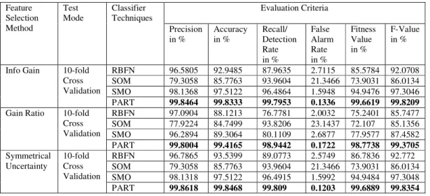
The performance of the proposed classification model that used RBF Network, Self-Organizing Map, Sequential Minimal Optimization and Projective Adaptive Resonance Theory as the classifiers and Info gain, Gain ratio and symmetrical uncertainty as the feature reduction methods was computed using various evaluation parameters such as precision, accuracy, recall, false alarm rate, fitness value, and F-value. For training and testing the standard 10-fold cross-validation technique was used. A comparative view of different combinations of classifiers and feature reduction techniques is depicted in table 4.
Table 4. Comparison of four ANN based classifiers using Entropy based feature selection.
Feature Selection Method Test Mode Classifier Techniques Evaluation Criteria Precision in % Accuracy in % Recall/ Detection Rate in % False Alarm Rate in % Fitness Value in % F-Value in %
Info Gain 10-fold
Cross Validation
RBFN 96.5805 92.9485 87.9635 2.7115 85.5784 92.0708
SOM 79.3058 85.7763 93.9604 21.3466 73.9031 86.0134
SMO 98.1368 97.5122 96.4864 1.5948 94.9476 97.3046
PART 99.8464 99.8333 99.7953 0.1336 99.6619 99.8209
Gain Ratio 10-fold
Cross Validation
RBFN 97.0904 88.1213 76.7781 2.0032 75.2401 85.7477
SOM 77.9224 84.7499 93.8206 23.1437 72.107 85.1356
SMO 96.2894 89.3064 80.1109 2.6877 77.9577 87.4582
PART 99.8004 99.4165 98.9442 0.1722 98.7738 99.3705
Symmetrical Uncertainty
10-fold Cross Validation
RBFN 96.7865 93.5399 89.0773 2.5749 86.7836 92.772
SOM 79.3058 85.7763 93.9604 21.3466 73.9031 86.0134
SMO 98.1318 97.5122 96.4915 1.5992 94.9484 97.3048
On comparison of results based on the evaluation criteria, Projective Adaptive Resonance Theory (PART) has the highest accuracy and detection rate and the lowest false alarm rate irrespective of the feature selection methods used. PART classification with symmetrical uncertainty feature selection gives the highest accuracy of 99.8468%, highest detection rate of 99.809% and lowest false alarm rate of 0.1203%. These results suggest that PART classification technique out performs other techniques, and thus more capable for intrusion detection as compared to other three techniques.
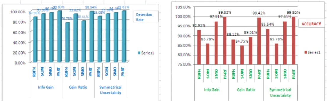
Accuracy, Recall/Detection Rate, False Alarm Rate, Precision, Fitness value, and F-Value of the classifiers with three entropy based feature selection methods are presented in Figures 5, 6, 7, 8, 9, 10 respectively.
Figure 5.Comparison of accuracy among the classifiersFigure 6. Comparison of detection rate among the classifiers
Figure 7.Comparison of false alarm rate among theclassifiersFigure 8. Comparison of precision among the classifiers
29
5.CONCLUSION
In this paper, different artificial neural network based classifiers along with three different entropy based attribute reduction methods were used to analyze the intrusion data and their performances were analyzed along different evaluation criteria. PART classification with symmetrical uncertainty feature selection gives the highest accuracy of 99.8468%, highest detection rate of 99.809%and lowest false alarm rate of 0.1203%. These results suggest that PART classification technique outperforms other techniques, and thus more suitable for building intrusion detection systems.
REFERENCES
[1] Mohammatreza Ektefa, Sara Memar, Fatimah Sidi, Lilly Suriani Affendey, “Intrusion detection using Data Mining Techniques”, Proceedings of IEEE International Conference on Information Retrieval & Knowledge Management, Exploring Invisible World, CAMP’ 10, pp. 200-203, 2010.
[2] Juan Wang; Qiren Yang; Dasen Ren, “An Intrusion Detection Algorithm Based on Decision Tree Technology”, Information Processing, APCIP, 2009, Asia-Pacific Conference, vol. 2, pp. 333-335,2009.
[3] Anazida Zainal, Mohd Aizaini Mariyam Shamsuddin, “Ensemble Classifiers for Network Intrusion Detection System”, Journal of Information, University Teknologi Malaysia, 2009.
[4] Sung, and S.Mukkamala. "The feature selection and intrusion detection problems" Advances in Computer Science-ASIAN 2004, Higher-Level Decision Making (2005): 3192-3193
[5] Lin Ni , Hong Ying Zheng “An Unsupervised Intrusion Detection Method Combined Clustering with Chaos Simulated Annealing” Proceeding of the Sixth International on Machine Learning and Cybernetics, Hong Kong, 19-22, August 2007
[6] Rung-Ching Chen, Kai-Fan Cheng and Chia-Fen Hsieh, “ Using Rough Set and Support Vector Machine for Network Intrusion Detection”, International Journal of Network Security and its Applications (IJNSA), Vol.1, No.1, 2009
[7] Amir Azimi, Alasti, Ahrabi, Ahmad Habibizad Navin ,Hadi Bahrbegi, “A New System for Clustering and Classification of Intrusion Detection System Alerts Using SOM”. International Journal of Computer Science & Security, vol:4, Issue:6, pp-589-597,2011
[8] P.J.Joseph, Kapil Vaswani, Matthew J, Thazhuthaveetil, “A Predictive Performance Model for Superscalar Processors Microarchitecture”, MICRO-39, 39thAnnual IEEE / ACM International Symposium, page: 161-170, Dec.2006.
[9] S.V. Chakravarthy and J.Ghosh, “Scale Based Clustering using Radial Basis Function networks”. Proceeding of IEEE International Conference on Neural Networks, Orlando, Florida, pp.897-902, 1994
[10] T. Kohonen, “The Self-Organizing Map”, Proceedings of the IEEE, Vol.78, Issue: 9, pp. 1464-1480, 1990.
[11] http://genome.tugraz.at/MedicalInformatics2/SOM.pdf
[12] J.Platt, “Fast Training of Support Vector Machines using Sequential Minimal Optimization” in Advances in Kernel Methods – Support Vector Learning, MIT Press, 1998.
[13] Y. Cao, J. Wu, “Projective ART for clustering data sets in high dimensional spaces”, Neural Networks, vol. 15, pp. 105-120, 2002.
[14] G. A. Carpenter “Distributed learning, recognition, and prediction by ART and ARTMAP neural networks”, Neural Networks, vol. 10, pp. 1473-1494, 1997.
[15] S.Grossberg, “Adaptive pattern classification and universal recording, Parallel development and coding of neural feature detectors”, Biological Cybernetics, vol. 23, pp. 121-134, 1976.