Abstract— In this paper, a new soft sensor methodology is proposed for estimation of product concentration in a chemical process. The new soft sensor utilizes dynamic principle component analysis (DPCA) method to select the optimum reduced process variables as the appropriate inputs. DPCA eliminates the high correlations among the process variable measurements, leading to a lower dimensional uncorrelated principle components of the process measurements. The DPCA transformed measurements are then used to train an adaptive growing and pruning radial basis function (GAP-RBF) neural network to estimate the product concentration. The developed soft sensor performance is demonstrated on a distillation column simulation case study.
Index Terms— dynamic principle component analysis, soft sensor, growing and pruning radial basis function neural network.
I. INTRODUCTION
Inferential estimators or soft sensors represent an attractive approach to estimate important primary process variables, particularly when conventional hardware sensors are not available, or when their high cost or technical limitations hamper their on-line use. Inferential estimators make use of easily available process knowledge, including a process model and measurements of secondary process variables, to estimate primary variables of interest [1]. In the process industries inferential estimators are typically used to estimate product compositions from the secondary variables.
It is well known that an inferential estimator can be developed in the form of a Luenberger observer [2] or a Kalman filter [3] using a first-principles dynamic model of the process. However, chemical processes are generally quite complex to model and are often characterized by significant inherent nonlinearities. As a consequence, inferential estimators are usually designed based on heuristic model of the process. For instance, the inferential estimator can be based on
Manuscript received July 22, 2007.
K. Amanian is with the Automation and Instrumentation Department, Petroleum University of Technology (e-mail: amaniankarim@ gmail.com).
K. Salahsoor is with the Automation and Instrumentation Department, Petroleum University of Technology (e-mail: [email protected]).
M. R. Jafari is with the Automation and Instrumentation Department, Petroleum University of Technology (e-mail:[email protected]).
M. Mosallaei is with the Automation and Instrumentation Department Petroleum University of Technology (e-mail: mohsenmosallaei@ gmail.com).
available measurements and multivariate regression techniques. This alternative approach for process variable estimation is advantageous because a soft sensor can provide a fast and accurate response, thus overcoming the typical limitations of hardware sensors [4]. Moreover, soft sensors are easy to develop and to implement online. Artificial neural networks (ANNs) are widely used estimation technique, and its successful application to the development of soft sensors for product composition estimation has already been reported for different processes [5]-[6].
It is not generally possible to overcome the issue of measurement selection difficulty by using all available secondary variables as soft sensor inputs, because measurement redundancy generally makes the calibration of the regression model troublesome and hence undermine the accuracy of the resulting estimator.
In this paper, a systematic measurement selection methodology is proposed and demonstrated in a simulated case study for a distillation process. 81 variables are used as secondary variables; the first 40 states are compositions of light component in different locations except the top production composition and the second 41 states are related to holdup information (state 42-82).The DPCA approach is applied for selecting the optimal inputs of the proposed soft sensor.
Principal component analysis (PCA) is a reliable and simple statistical technique for handling high dimensional, noisy, and correlated measurement data by projecting the data onto a lower dimensional subspace which contains most of the variance of the original data [7]. Considering the limitation of the conventional PCA, dynamic PCA (DPCA) has been utilized in this paper to increase the accuracy of selecting optimal sensor inputs. DPCA does this task by extracting time-dependent relationship in the measurement through augmenting the measured data matrix by time lagged measured variables. The DPCA transformed data are then applied to the soft sensor as the optimal inputs from the uncorrelated statistical perspective. The growing and pruning radial basis function (GAP-RBF) neural network introduction in [8] is modified to enable the on-line estimation of the unknown concentration. The unscented kalman filter (UKF) has been developed as an efficient learning algorithm for the modified GAP-RBF neural network.
The rest of this paper is organized as follows. Section II (A) presents the DPCA algorithm. Section II (B) introduces the original GAP-RBF neural network. A modified GAP-RBF
Soft Sensor Based on Dynamic Principal
Component Analysis and Radial Basis Function
Neural Network for Distillation Column
neural network is presented in section II (C) to improve its performance for on-line soft sensor application. The UKF learning algorithm it’s introduced in section II (D) to update the free parameters of the modified GAP-RBF neural network. The performance of the proposed soft sensor is demonstrated in section III to estimate the product concentration of a distillation column benchmark problem. Section IV and V summarizes the resulting observations and conclusions.
II. PROPOSED METHODOLOGY
A. DPCA algorithm
Consider a typical process with m observations of n process variables. The measured data can be organized in a data matrix (X) with (
m
×
n
) dimension. Computationally, PCA transforms the data matrix X by combining the variables as a linear weighed sum as follows:∑
=≅
=
α 1 i T i i TP
t
TP
X
(1) wheret
i is a score vector which contains information about relation between samples, andp
i is a loading vector which contains information about relationship between variables. Note that score vectors are orthogonal and loading vectors are orthonormal. Projection into principle component space reduces the original set of variables (n) toα
latent variables. That is, projections of the measured variables are done along the directions determined by the k eigenvectors{
p
1,
p
2,...,
p
} (k<n) corresponding to first k largesteigenvalues of the covariance matrix of X. Thus, by discarding those principal components that do not contribute significantly to overall variation, the dimensionality of the problem is correspondingly reduced. PCA algorithm, however, is best suited for analysis of steady state data with uncorrelated measurements. The steady state PCA approach can be extended to dynamic process by DPCA. By augmenting the sample vector and including time-lagged measured variables as:
)]
(
)...
1
(
),
(
[
)
(
t
M
t
M
t
M
t
l
X
=
−
−
(2)
where M (t) is the vector of measurements, standing for the current time; while the DPCA determines the proper number of
l and the principal components, which indicate the order of the
process. The dynamic model which can be extracted from the measured data is an implicitly multivariate auto-regressive (AR) model.
B. GAP-RBF Neural Network
GAP-RBF neural network uses the Gaussian RBF network (GRBF). Its output vector f (xn), which approximates the
desired output vector
y
n, are described as follows:∑
==
K k n k k nx
x
f
1)
(
)
(
α
φ
(3) whereα
kis its connecting weight to the output neuron, and)
(
nk
x
φ
denotes a response of the kth hidden unit to the inputs)
(
;
k nn
x
x
φ
is a Gaussian function given by:⎟
⎟
⎠
⎞
⎜
⎜
⎝
⎛
−
−
=
2 2exp
)
(
k k n n kx
x
σ
μ
φ
(4)where
μ
kandsσ
k are the center and width of the Gaussian function respectively, and.
denotes the Euclidean norm.The original GAP-RBF neural network [8] employs a sequential learning algorithm for training during the sequential learning process, a series of training samples (
x
i, y (x
i)); (i =1, 2...) are randomly drawn and presented one by one to the
network. Each training data sample may trigger the action of adding a new hidden neuron, pruning the nearest hidden neuron, or adjusting the free parameters of the nearest hidden neuron, based on the significance of the nearest hidden neuron to the training data sample. The significance of the kth hidden neuron is defined as [8]:
)
(
)
8
.
1
(
)
(
X
S
k
E
k l k sigα
σ
=
(5)where l is the dimension of the input space
x
n∈
R
l, andS(X) denotes the estimated size of the range X where the
training samples are drawn from.
Given the set of all hidden neuron in A, only the nearest neuron based on the following Euclidean distance to the current input data xn is checked for its significance:
))}
(
min
(
)
(c
{
,..., 1 r i K i rr
A
x
c
x
c
∈
∨
−
=
−
μ
= (6)
where
c
ris the center of the hidden neuron which is nearest to xn.The learning process of the GAP-RBF network begins with no initial hidden neurons. As new observation data (xn,yn) are
received during the training, some of them may initiate new hidden neurons based on the following growing criterion:
min min
)
(
)
8
.
1
(
e
X
S
e
c
x
e
e
c
x
n l r n n n r nf
f
f
−
−
κ
ε
(7)where emin is the desired approximation accuracy,
ε
nis athreshold to be selected appropriately, and en=yn-f(xn). If the
growing criterion is satisfied, than a new neuron (K+1) will be added whose tuning parameters are set as follows:
nr n K n K n K
x
x
e
μ
κ
σ
μ
α
−
=
=
=
+ + + 1 1 1 (8)However, if a new observation (xn, yn) arrivers and the
)
,
,
(
α
nrμ
nrσ
nr will be adjusted using the EKF learningalgorithm. Similarly, as the training carries on, some of the new observations (xn,yn) may trigger the learning algorithm to prune
some hidden neurons. The pruning criterion is based on the significance of the nearest neuron to the new observation, as follows: min
)
(
)
8
.
1
(
)
(
e
X
S
k
E
k l k sigp
α
σ
=
(9)If the above average contribution made by the nearest neuron in the whole range X is less than the expected accuracy emin,
then the nearest neuron is removed. The complete description of the GAP-RBF learning algorithm can be summarized as follows [8]:
Given an approximation error emin, for each new observation
)
,
(
x
R
ly
nR
n
∈
∈
the following steps are performedsequentially:
1. Compute the overall network output:
⎟
⎟
⎠
⎞
⎜
⎜
⎝
⎛
−
−
=
∑
= 2 2 1exp
)
(
k k n K k k nx
x
f
σ
μ
α
(10)where K is the number of hidden neurons.
2. Calculate the required parameters for the growth criterion:
)
(
)
1
0
(
},
,
{
max
max minn n n n n
x
f
y
e
=
−
=
ε
γ
ε
p
γ
p
ε
(11) 3. If the growth criterion, specified by (7), is satisfied, allocate a new hidden neuron K+1 with tuning parameters given by (8).
. . .
Else
4. Adjust the neural network parameters for the nearest neuron only
(
α
nr,
μ
nr,
σ
nr)
using the EKF estimation algorithm.5. Check the pruning criterion for the nearest hidden neuron, described by (9). It Esig(nr)<emin, remove the nearest hidden
neuron and do the necessary network parameter adaptation by the EKF algorithm.
Endif Endif
C. The modified GAP-RBF neural network
In order to have smoothly output response and avoid oscillation, the mechanism of adding and pruning should be modified. The rate of adding or pruning of neurons can be controlled with threshold values of
e
nandε
n . Selection of these values depends on the complexity of the process, input data for identification and the required accuracy for the model. But the most important and effective factor is the persistent exciting (PE) of the input data. If the input data have enough degree of PE, smooth and accurate output can be obtained with suitable adjusting of the threshold values, but if the inputs do not possess PE, which may happen for instance in the case of closed-loop identification, then the threshold values can nothelp and hence modification on adding and pruning rules will be necessary.
In on-line identification, it should be better to change the adding strategy in such a way that, the rate of adding neurons increased in the beginning of the identification process, and as the identification process continues on, the rate of adding neurons is decreased. In the original algorithm [8], and its applications [8]-[9]-[10], neurons are added hardly in the start of the modeling process. This causes large errors in the start of the algorithm. As the rate of neuron creation can be controlled with
ε
n , an exponential function is proposed to be used in order to changeε
n with time evolution as follows.)
1
)(
(
max minmin
ε
ε
τε
ε
n ne
−−
−
+
=
(12) whereτ
is the parameter that can be used to control the changing rate ofε
n.Another problem is due to oscillation in the number of created neurons that can cause big errors in the identification results. This oscillation will be occurred in on-line identification, when the number of neurons that are created are small and the input data have small degree of PE, too. The effects of mentioned problem can be reduced with changing the pruning criteria by adding a new pruning factor
(
β
)
as follows: min ) ()
8
.
1
(
e
X S nr lnr
α
β
σ
p
(13)D. The UKF Learning Algorithm
The original GAP-RBF neural network presented in [8] uses the EKF learning algorithm. This algorithm, however, may diverge if the consecutive linearization of the nonlinear process model around the last state estimate dose not give a good approximation. The inherent flows of the EKF due to its linearization approach for calculating the mean and covariance of a random variable which undergoes a nonlinear transformation are addressed by the UKF algorithm [12]. This is done by utilizing a deterministic sampling approach to calculate mean and covariance terms.
Essentially, 2L+1 sigma points (L is the state dimension) are chosen based on a square-root decomposition of the prior covariance. These sigma points are propagated through the true nonlinearity, without approximation, and then a weighted mean and covariance is taken. This approach results in approximations that are accurate to the third order (Taylor series expansion) for Gaussian inputs for all nonlinearities.
In on-line estimation the learning algorithms should be fast. In this paper, the following useful way of rationalizing this desired objective has been presented to modify the covariance matrix update relationship:
k T k y y k k
k
p
k
p
k
p
k
k
)
/
η
(
−
=
−(14) where Kk represents the kalman gain and
P
ykykdenote themeasurement covariance matrix.
which undergoes the following time-vary evolution:
1
0
;
)
1
)(
1
(
11
+
−
−
<
≤
=
− − − kt
k k
k
η
η
e
η
η
δ (15)Where t is the recursive time interval that is spent in the modified UKF learning algorithm to estimate the modified GAP-RBF neural network free parameters with fixed dynamic structure. Thus, t is reset to zero when any network structural change, i.e., neuron creation or pruning occurs. This scheme maintains a desired parameter adaptive capability in the modified UKF algorithm whenever process dynamics undergoes a time-varying change.
η
kstarts with a lower initial value to accelerate the parameter estimation and is then changed exponentially with a desired time-constant (δ
) to a higher final value to assure the estimator convergence property.III. SIMULATION CASE STUDY
In this section, a distillation column benchmark problem [11] has been used to evaluate the performance of the proposed soft sensor methodology to estimate the column top product concentration. The distillation column, shown in Fig. (1), consist of four manipulated inputs (LT, VB, D and B), three disturbances (F, zF and qF) and 82 states. Assuming that the top product composition (i.e., the column state number 31) as the unknown variable, its behavior is intended to be estimated by the proposed soft sensor. All the 81 states are used as the input data matrix to the DPCA algorithm. Then, the first 4 eigenvectors corresponding to the first 4 largest eigenvalues of the covariance data matrix are utilized as the selected principle components to reduce the high dimensionality of the problem. These states including their four time-lagged information are used as the input data matrix to the soft sensor. The DPCA transformed data, that is the projection of the original high dimensional input data on the chosen four principle component space are used to train the modified GAP-RBF neural network in an online manner.
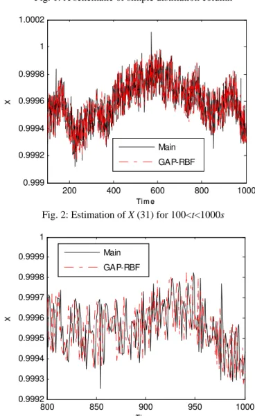
The collected column data samples were then used for online estimation. Fig. (2) demonstrates the performance of the online soft sensor .For more clarity , the resulting performance has been illustrated for a shorter time interval of 800 to1000 data samples. As it is shown, the soft sensor is able to estimate the real top product composition with high accuracy. This result can be verified quantitatively by the integral of squared error (ISE) measure which is equal to 1.9982 for the whole time interval.
IV. SIMULATION RESULTS
In this section, we apply DPCA to distillation column as case study then the identification capability of the modified GAP-RBF neural network is tested on non-linear benchmark problem [11].We use Distillation Column (Skogestad Model) for Implementation of our methods .
Fig. 1: A schematic of simple distillation column
200 400 600 800 1000 0.999
0.9992 0.9994 0.9996 0.9998 1 1.0002
Ti m e
X
Main GAP-RBF
Fig. 2: Estimation of X (31) for 100<t<1000s
800 850 900 950 1000 0.9992
0.9993 0.9994 0.9995 0.9996 0.9997 0.9998 0.9999 1
Ti m e
X
Main GAP-RBF
Fig. 3: Estimation of X (31) for arbitrary time V. CONCLUSIONS
elimination of the high correlations among the process measured secondary variables leading to low dimensional uncorrelated transformed data. An adaptive modified GAP-RBF neural network has been trained on-line to estimate the unknown column top product composition based on the DPCA transformed data feature. A modified UKF learning algorithm, including a forgetting factor strategy, has been presented to estimate the free adoptive neural network parameters. The resulting soft sensor methodology has been evaluated on a distillation column benchmark problem. The obtained observations are promising and demonstrate the accurate performance of the proposed methodology to estimate the distillation column top product.
REFERENCES
[1] C. Brosilow, B. Joseph, “Techniques of Model Based Control”, Prentice
Hall, New York, USA, 2002.
[2] D.C. Luenberger, “Observing the state of a system”, IEEE Trans. Military Electron. MIL-8, 74–80, 1964.
[3] R.E. Kalman, “A new approach to linear filtering and prediction problems”, Trans. ASME, J. Basic Eng. 82, 35–45, 1960.
[4] H. Leegwater, “Industrial experience with double quality control”, in: W.L. Luyben (Ed.), Practical Distillation Control, Van Nostrand Reinhold, New York, USA, 1992.
[5] T. Kourti, J.F. MacGregor, Tutorial: “Process analysis, monitoring and diagnosis, using multivariate regression methods”, Chemom. Intell. Lab. Syst. 28, 3-21, 1995.
[6] S.J. Qin, “Neural network for intelligent sensors and control––practical issues and some solutions”, in: O. Omidvar, D.L. Elliott (Eds.), Neural Systems for Control, Academic Press, New York,USA, 1997.
[7] L. I. Smith, “A tutorial on Principal Components Analysis”,February 26, 2002
[8] G.-B Huang., P. Saratchandran, and N. Sundararajan,“An efficient sequential learning algorithm for Growing and Pruning RBF (GAP-RBF) networks” IEEE Transactions on systems, man, and cybernetics, part B, vol. 34, No. 6,December 2004.
[9] G.B. Huang, P. Saratchandran, and N. Sundararajan,“A generalized growing and pruning RBF (GGAP-RBF) neural network for function approximation,” IEEE Trans. Neural Networks, vol. 16, No. 1, January 2005.
[10] Y. Wang, G.-B. Huang, P. Saratchandran, and N. Sundararajan, “Time Series Study of GGAP-RBF Network: Predictions of Nasdaq Stock and Nitrate Contamination of Drinking Water”, Proceedings of International
Joint Conference on Neural Networks, Montreal, Canada, July 31 -
August 4, 2005.
[11] T. Mejdell; S. Skogestad, “Output estimation using multiple secondary measurements: High-Purity Distillation”. AIChE J., 39(10), 1641-1653, 1993.