Feature Selection via Chaotic Antlion
Optimization
Hossam M. Zawbaa1,2*, E. Emary3,4, Crina Grosan1,5
1Faculty of Mathematics and Computer Science, Babes-Bolyai University, Cluj-Napoca, Romania,2Faculty of Computers and Information, Beni-Suef University, Beni-Suef, Egypt,3Faculty of Computers and Information, Cairo University, Cairo, Egypt,4Faculty of Computer Studies, Arab Open University, Cairo, Egypt,5College of Engineering, Design and Physical Sciences, Brunel University, London, United Kingdom
Abstract
Background
Selecting a subset of relevant properties from a large set of features that describe a dataset is a challenging machine learning task. In biology, for instance, the advances in the available technologies enable the generation of a very large number of biomarkers that describe the data. Choosing the more informative markers along with performing a high-accuracy classifi-cation over the data can be a daunting task, particularly if the data are high dimensional. An often adopted approach is to formulate the feature selection problem as a biobjective optimi-zation problem, with the aim of maximizing the performance of the data analysis model (the quality of the data training fitting) while minimizing the number of features used.
Results
We propose an optimization approach for the feature selection problem that considers a “chaotic”version of the antlion optimizer method, a nature-inspired algorithm that mimics the hunting mechanism of antlions in nature. The balance between exploration of the search space and exploitation of the best solutions is a challenge in multi-objective optimization. The exploration/exploitation rate is controlled by the parameterIthat limits the random walk range of the ants/prey. This variable is increased iteratively in a quasi-linear manner to decrease the exploration rate as the optimization progresses. The quasi-linear decrease in the variableImay lead to immature convergence in some cases and trapping in local min-ima in other cases. The chaotic system proposed here attempts to improve the tradeoff between exploration and exploitation. The methodology is evaluated using different chaotic maps on a number of feature selection datasets. To ensure generality, we used ten biologi-cal datasets, but we also used other types of data from various sources. The results are compared with the particle swarm optimizer and with genetic algorithm variants for feature selection using a set of quality metrics.
OPEN ACCESS
Citation:Zawbaa HM, Emary E, Grosan C (2016) Feature Selection via Chaotic Antlion Optimization. PLoS ONE 11(3): e0150652. doi:10.1371/journal. pone.0150652
Editor:Josh Bongard, University of Vermont, UNITED STATES
Received:August 25, 2015
Accepted:February 16, 2016
Published:March 10, 2016
Copyright:© 2016 Zawbaa et al. This is an open access article distributed under the terms of the
Creative Commons Attribution License, which permits unrestricted use, distribution, and reproduction in any medium, provided the original author and source are credited.
Data Availability Statement:Datasets are downloaded from the UCI Machine Learning Repository, [http://archive.ics.uci.edu/ml]. Irvine, CA: University of California, School of Information and Computer Science, 2013.
1 Introduction
The large amounts of data generated today in biology offer more detailed and useful informa-tion on the one hand, but on the other hand, it makes the process of analyzing these data more difficult because not all the information is relevant. Selecting the relevant characteristics or attributes of the data is a complex problem. Feature selection (attribute reduction) is a tech-nique for solving classification and regression problems, and it is employed to identify a subset of the features and remove the redundant ones. This mechanism is particularly useful when the number of attributes is large and not all of them are required for describing the data and for further exploring the data attributes in experiments. The basic assumption for employing fea-ture selection is that a large number of feafea-tures do not necessarily translate into high classifica-tion accuracy for many pattern classificaclassifica-tion problems [1]. Ideally, the selected feature subset will improve the classifier performance and provide a faster and more cost effective classifica-tion, which leads to comparable or even better classification or regression accuracy than using all the attributes [2]. In addition, feature selection improves the visualization and the compre-hensibility of the induced concepts [3]. Using a tumor as a simple example, there are a large number of attributes that describe it: mitotic activity, tumor invasion, tumor shape and size, vascularization, and growth rate, to name just a few. All of these attributes require measure-ments and tests that are not always easy to perform. Thus, it will be ideal if the classification of a tumor into benign or malignant (and which stage) could be performed with fewer investiga-tions. The selection of a subset of the features that are relevant enough to perform the classifica-tion will be of considerable benefit.
Many studies formulate the feature selection problem as a combinatorial optimization lem, in which the selected feature subset leads to the best data fitting [4]. In real world prob-lems, feature selection is mandatory due to the abundance of noisy, irrelevant or misleading features [5]. These factors can have a negative impact on the classification performance during the learning and operation processes. Two main criteria are used to differentiate the feature selection methods:
1. Search strategy: the method employed to generate feature subsets or feature combinations.
2. Subset quality (fitness): the criteria used to judge the quality of a feature subset.
There are two main classes of feature selection methods: wrapper-based methods (apply machine learning algorithms) and filter-based methods (use statistical methods) [6].
Thewrapper-based approachuses a machine learning technique as part of the evaluation function, which facilitates obtaining better results than the filter-based approach [7], but it has a risk of over-fitting the model and can be computationally expensive, and hence, a very intelli-gent search method is required to minimize the running time [8]. In contrast, thefilter-based approachsearches for a subset of features that optimize a given data-dependent criterion rather than classification-dependent criteria as in the wrapper methods [1].
In general, the feature selection problem is formulated as a multi-objective problem with two objectives: minimize the size of the selected feature set and maximize the classification accuracy. Typically, these two objectives are contradictory, and the optimal solution is a trade-off between them.
The size of the search space exponentially increases with respect to the number of features in the dataset [8]. Therefore, an exhaustive search for obtaining the optimal solution is almost impossible in practice. A variety of search techniques have been employed, such as greedy search based on sequential forward selection (SFS) [9] and sequential backward selection (SBS) [10]. However, these feature selection approaches still suffer from stagnation in local optima and expensive computational time [11]. Evolutionary computing (EC) algorithms and other
collection and analysis, decision to publish, or preparation of the manuscript.
population-based algorithms adaptively search the feature space by employing a set of search agents that communicate in a social manner to reach a global solution [12]. Such methods include genetic algorithms (GAs) [13], particle swarm optimization (PSO) [14], and ant colony optimization (ACO) [3].
GAs and PSO are the most common population-based algorithms. GAs are inspired from the process of evolution via natural selection and survival of the fittest and have the ability to solve complex and non-linear problems; however, in many cases, if no additional mechanisms are employed, they can have poor performance and become trapped in local minima [15]. In PSO, each solution is considered as a particle that is defined by position, fitness, and a speed vector, which defines the moving direction of the particle [16].
The antlion optimization (ALO) algorithm [17] is a relatively recent algorithm that is com-putationally less expensive than other techniques. The chaotic optimization algorithm (COA) is a global optimization method whose main core contains two phases [18]. The first phase has four steps:
1. Produce a sequence of chaotic points;
2. Map the chaotic points to a sequence of design points in the design space;
3. Compute the fitness (objective function) values based on the design points;
4. Select the point that has the minimum fitness value as the current optimum point.
The second phase has two steps:
1. Assume that the current optimum point is located near the global optimum after a number of iterations;
2. Perform position alteration and search around the current optimum in the descent direction along with the axis directions.
These phases are repeated until a convergence (termination) criterion is met. Chaos is con-sidered to be a deterministic dynamic process and is very responsive to its initial parameters and conditions. The nature of chaos is clearly random and unpredictable, but it also has an ele-ment of regularity [18].
The aim of this paper is to enhance the performance of the antlion optimizer for feature selection by using chaos. We are particularly interested in applying our methods to data from biology and medicine, as these data possess a large number of attributes and generally have a small number of instances, which makes the feature selection process more complex.
The remainder of this paper is organized as follows. Subsection 1.1 surveys the existing related work. Section 2 provides background information about the antlion optimization algo-rithm and chaotic maps. The proposed chaotic version of the antlion optimization (CALO) is presented in Subsection 2.3. The experimental results with discussions are reported in Section 3. The conclusions of this research and directions for future work are presented in Section 4.
1.1 Related work
An ACO-based wrapper feature selection algorithm has been applied in network intrusion detection [22]. ACO uses the Fisher discrimination rate to adopt the heuristic information. A feature selection method based on ACO and rough set theory has been proposed in [23]. Logis-tic map is one of the techniques used by the chaoLogis-tic behavior and has bounded unstable dynamic behavior. The system proposed in [24] uses the K-nearest neighbor (KNN) classifier with leave-one-out cross-validation (LOOCV) and evaluates the classification performance.
The chaos genetic feature selection optimization method (CGFSO) is proposed in [18]. The method proposed in [25] for text categorization consists of some primary stages, such as fea-ture extraction and feafea-ture selection. In the feafea-ture selection stage, the method applies feafea-ture selection algorithms to obtain a feature subset that can increase the classification accuracy and method performance and can reduce the learning complexity. CGFSO explores the search space with all possible combinations of a given dataset. In addition, each individual in the pop-ulation represents a candidate solution, with the size of the feature subset being the same as the length of a chromosome [26].
Chaotic time series with the EPNet algorithm is proposed in [27]. The authors present four different methods derived from the classical EPNet algorithm applied in three different chaotic series (Logistic, Lorenz, and Mackey-Glass). The tournament EPNet algorithm obtains the best results for all time series considered, and the network architectures remains of a comparatively limited size. The chaotic time series predictor requires a small network architecture, whereas the addition of neural components may degrade the performance during evolution and conse-quently provide more survival probabilities to smaller networks in the population [28].
2 Methods
2.1 Antlion optimization (ALO)
Antlion optimization (ALO) is a bio-inspired optimization algorithm proposed by Mirjalili [17]. The ALO algorithm mimics the hunting mechanism of antlions in nature. Antlions (doo-dlebugs) belong to the Myrmeleontidae family and Neuroptera order [17]. They primarily hunt in the larvae stage, and the adulthood period is for reproduction. An antlion larvae digs a cone-shaped hole in the sand by moving along a circular path and throwing out sand with its huge jaw. After digging the trap, the larvae hides underneath the bottom of the cone and waits for insects/ants to become trapped in the hole. Once the antlion realizes that a prey is in the trap, it attempts to catch the prey. However, insects are typically not caught immediately and attempt to escape from the trap.
In this case, antlions intelligently throw sand toward the edge of the hole to cause the prey to slide to the bottom of the hole. When a prey is caught in the jaw of an antlion, it is pulled under the soil and consumed. After consuming the prey, antlions throw the leftovers outside the hole and prepare the hole for the next hunt.
Artificial antlion. Based on the above description of antlions, Mirjalili uses the following facts and assumptions in the artificial antlion optimization algorithm [17]:
• Prey (ants) move around the search space using different random walks;
• Random walks are affected by the traps of antlions;
• Antlions can build holes proportional to their fitness (the higher the fitness, the larger the hole);
• Antlions with larger holes have a higher probability of catching ants;
• The range of random walks is decreased adaptively to simulate sliding ants toward antlions;
• If an ant becomes fitter than an antlion, this means that the ant is caught and pulled under the sand by the antlion;
• An antlion repositions to the most recently caught prey and builds a hole to improve its chance of catching another prey after each hunt.
Formally, the antlion optimization algorithm is given in Algorithm 1.
Algorithm 1:Antlion optimization (ALO) algorithm
Input:Search space, fitness function, numbers of ants and antlions, number of iterationsT
Output:The elitist antlion and its fitness
1. Randomly initialize a population of ant positionsAntand a population of antlion positionsAntlion.
2. Calculate the fitness of all the ants and antlions. 3. Find the fittest antlion; Elite.
4.t= 0.
5.while(tT) foreachAntido
•Select an antlion using Roulette wheel. •Slide ants toward the antlion as inEq (2).
•Create a random walk for theAntiand normalize it, as shown in Eqs (4)
and (5) for modeling trapping,Eq (6)for random walk, andEq (8)for walk normalization.
end
6. Calculate the fitness of all ants.
7. Replace an antlion with its corresponding ant if the ant becomes fitter followingEq (1).
8. Update the elite if an antlion becomes fitter than the current elite. 9.t=t+1
end while
The antlion optimizer applies the following steps to an individualantlion:
1. Building a trap:a roulette wheel is used to model the hunting capability of antlions. Ants are assumed to be trapped in only oneselectedantlion hole. The ALO algorithm requires a roulette wheel operator for selecting antlions based on their fitness during optimization. This mechanism provides high chances to the fitter antlions for catching prey or ants.
2. Catching prey and re-building the hole:this is the final stage in hunting, in which the antlion consumes the ant. It is assumed that prey catching occurs when the ant becomes fit-ter (goes inside sand) than its corresponding antlion. The antlion has to update his position to the latest position of the hunted ant to increase its chance of catching new prey.Eq (1) reflects this process:
Antliont
j ¼Antit If fðAntitÞ is better than fðAntliontjÞ; ð1Þ
where:
• tshows the current iteration;
• Antliont
jshows the position of the antlionjat iterationt;
• Antt
iindicates the position of the antiat iterationt.
1. Sliding ants toward antlion:antlions shoot sand toward the center of the hole once they realize that an ant is in the trap. This behavior causes the trapped ant that is attempting to escape to slide down. To mathematically model this behavior, the radius of the ants’random walk hyper-sphere isdecreasedadaptively using Eqs (2) and (3).
ct ¼c t
I; ð2Þ
where:
• ctis the minimum of all variables at iterationt;
• Iis a ratio, which is defined inEq (3):
I¼10w t
T; ð3Þ
where:
• tis the current iteration;
• Tis the maximum number of iterations;
• wis a constant defined based on the current iteration (w= 2 whent>0.1T,w= 3 when t>0.5T,w= 4 whent>0.75T,w= 5 whent>0.9T, andw= 6 whent>0.95T). Basically, the constantwcan adjust the accuracy level of exploitation.
2. Trapping in the antlion holes:by modeling the sliding of prey toward the antlion, the ant is trapped in the antlion’s hole. In other words, the walk of the ant becomes bounded by the position of the antlion, which can be modeled by changing the range of the ant random walk toward the antlion position as in Eqs (4) and (5):
ct
i ¼ctþAntliontj; ð4Þ
dt
i ¼dtþAntliontj; ð5Þ
where:
• ctis the minimum of all variables at iterationt;
• dtis the maximum of all variables at iterationt;
• ctiis the minimum of all variables for anti;
• dt
iis the maximum of all variables for anti;
• Antliont
jrepresents the position of the antlionjat iterationt.
3. Random walks of ants:Random walks are based onEq (6):
XðtÞ ¼ ½0;cumsumð2rðt1Þ 1Þ;cumsumð2rðt2Þ 1Þ; :::;cumsumð2rðtTÞ 1Þ;
ð6Þ
where:
• cumsumcalculates the cumulative sum;
• Tis the maximum number of iterations;
• r(t) is a stochastic function defined as:
rðtÞ ¼
1 if rand>0:5
0 if rand0:5; (
ð7Þ
whererandis a random number generated with a uniform distribution over [0, 1].
To keep the random walks inside the search space, they are normalized usingEq (8)(min–max normalization):
Xt i ¼
ðXt
i aiÞ ðdi c t iÞ
ðbt i aiÞ
þci; ð8Þ
where:
• aiis the minimum random walk for variablei;
• biis the maximum random walk for variablei;
• ctiis the minimum of variableiat iterationt;
• ditis the maximum of variableiat iterationi.
4. Elitism:to maintain the best solution(s) across iterations, elitism has to be applied. In this work, we consider that the random walk of an ant is guided by the selected antlion and by the elite antlion, and hence, the repositioning of a given ant follows the average of both ran-dom walks, as shown inEq (9):
Antt i ¼
Rt AþRtE
2 ; ð9Þ
where:
• Rt
Ais the random walk around the antlion selected using a roulette wheel;
• Rt
Eis the random walk around the elite antlion.
2.2 Chaotic maps
Chaos means a condition or place of great disorder or confusion [29]. Chaotic systems are deterministic systems that exhibit irregular (or even random) behavior and a sensitive depen-dence on the initial conditions. Chaos is one of the most popular phenomena that exist in non-linear systems, whose action is complex and similar to that of randomness [30]. Chaos theory studies the behavior of systems that follow deterministic laws but appear random and unpre-dictable, i.e., dynamical systems. To be referred to as chaotic, the dynamical system must satisfy the following chaotic properties [29]:
1. sensitive to initial conditions;
2. topologically mixing;
3. dense periodic orbits;
4. ergodic;
5. stochastically intrinsic.
chaos search is more capable of hill-climbing and escaping from local optima than random search, and thus, it has been applied for optimization [30]. It is widely recognized that chaos is a fundamental mode of motion underlying almost all natural phenomena. A chaotic map is a map that exhibits some type of chaotic behavior [29]. The common chaotic maps in the litera-ture are as follows:
1. Logistic map:this map is one of the simplest chaotic maps [31], as defined inEq (10):
xkþ1 ¼axkð1 xkÞ; ð10Þ
where:
• xk2(0, 1) under the condition thatx02[0, 1], 0<a4; • kis the iteration number.
2. Sinusoidal map:represented byEq (11)[31]:
xkþ1¼ax2ksinðpxkÞ; ð11Þ
which generates chaotic numbers in the range (0, 1) witha= 2.3.
3. Tent map:resembles the logistic map due to its topologically conjugate behavior. A tent map can display a range of dynamical behaviors from predictable to chaotic depending on the value of its multiplier, as shown in Eqs (12) and (13):
xkþ1¼GðxkÞ; ð12Þ
GðxÞ ¼
x
0:7; x<0:7
1
0:3xð1 xÞ otherwise 8 > > < > > :
ð13Þ
4. Singer map:given inEq (14)[32]:
xkþ1¼mð7:86xk 23:31x
2
kþ28:75x
3
k 13:3x
4
kÞ; ð14Þ
withxk2(0, 1) under the condition thatx02(0, 1),μ2[0.9, 1.08].
5. Piecewise map:given inEq (15)[33]:
xkþ1¼ x
p; 0xk<p xk p
0:5 p pxk<0:5
1 p xk
0:5 p 0:5xk<ð1 pÞ
1 xk
p ð1 pÞ xk<1
8 > > > > > > > > > > > > > > < > > > > > > > > > > > > > > :
ð15Þ
2.3 The novel chaotic antlion optimization (CALO)
In this section, we present our chaotic antlion optimization (CALO) algorithm based on k-nearest neighbor (KNN) for feature selection.Explorationcan be defined as the acquisition of new information through searching [34]. Exploration is a main concern for all optimizers because it might lead to new search regions that might contain better solutions.Exploitationis defined as the application of known information. The good sites are exploited via the applica-tion of a local search. The selecapplica-tion process should be balanced between random selecapplica-tion and greedy selection to bias the search toward fitter candidate solutions (exploitation) while pro-moting useful diversity into the population (exploration) [34].
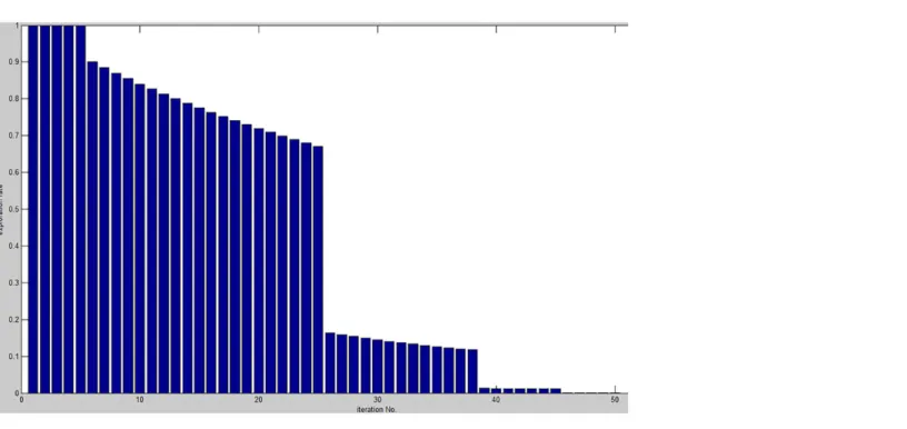
ParameterIcontrols the trade-off between exploration and exploitation in the original antlion optimization algorithm. This parameter is linearly decreased to allow more exploration at the beginning of the optimization process, while exploitation becomes more important at the end of the optimization. Therefore, half of the optimization resources are consumed in exploration, whereas the remaining time is dedicated to exploitation, as shown in (Fig 1).
Although the algorithm proved efficient for solving numerous optimization problems, it still possesses the following drawbacks:
1. Sub-optimal selection:at the beginning of the optimization process,Iis small, which makes the random walk unbounded in the search space and allows an ant to apply random walk in almost the entire search space. This may cause the algorithm to select sub-optimal solutions.
2. Stagnation:once the algorithm approaches the end of the optimization process, it becomes difficult to escape local optima and find better solutions because its exploration capability is very limited;Ibecomes very large, thereby limiting the boundaries for the random walk. This causes the algorithm to continue enhancing solutions that have already been found, even if they are sub-optimal.
Fig 1. Exploration rate (1
These problems motivate our work on adapting1
Ito obtain successive periods of exploration
and exploitation. Therefore, when reaching a solution, exploitation will be applied, followed by another exploration, which may jump to another promising area, followed by using exploitation again to further enhance the solution found, and so on. Chaotic systems with their interesting properties, such as topologically mixing and dense periodic orbits, ergodicity and intrinsic sto-chasticity, can be used to adapt this parameter, allowing for the required mix between explora-tion and exploitaexplora-tion. (Fig 2a) presents an example of a chaos map for the values ofIfor 500 iterations, in which we can observe alternating regions of exploration and exploitation. A small variation in the period means exploitation, whereas a larger variation in the period means explo-ration. Thetentmap smoothly and periodically decrements the exploration rate, while the sinu-soidal map abruptly switches between exploration and exploitation, which may cause loss of the optimal solution and lead to worse performance (as shown in (Fig 2b and 2c).
The proposed CALO algorithm is schematically presented in (Fig 3). The search strategy of the wrapper-based approach explores the feature space to find a feature subset guided by the classification performance of individual feature subsets.
This approach may be slow because the classifier must be retrained on all the candidate sub-sets of the feature set and its performance must be measured. Therefore, an intelligent search of the feature space is required. The goals are to maximize the classification performancePand to minimize the number of selected featuresNf. The fitness function is given inEq (16)[35]:
minimize að1 PÞ þ ð1 aÞ Nf
Nt
; ð16Þ
where:
• Nfis the size of the selected feature subset;
• Ntis the total number of features in the dataset;
• α2[0, 1] defines the weights of the sub-goals;
• Pis the classification performance measured as inEq (17).
P¼Nc
N ; ð17Þ
whereNcis the number of correctly classified data instances andNis the total number of instances in the dataset.
The number of dimensions in the optimization is the same as the number of features, with each feature related to a dimension and each variable limited to the range [0, 1]. To determine whether a feature will be selected at the evaluation stage, a static threshold of 0.5 is used, as Fig 2. The exploration and exploitation values of different chaotic maps.
shown inEq (18):
yij¼
0 Ifðxij<0:5Þ
1 Otherwise (
ð18Þ
whereyijis the discrete representation of solution vectorx, andxijxijis the continuous position of the search agentiin dimensionj.
3 Results and Discussion
3.1 Experimental setup
Datasets. Table 1summarizes the 18 datasets used for the experiments. The datasets are taken from the UCI data repository [36]. We use ten biological datasets to validate the perfor-mance of our method and its potential applicability for data generated in biology. In addition, we use eight datasets from other areas to show the general adaptability of our method. Each dataset is divided into 3 equal parts fortraining,validation, andtesting. Thetrainingset is used to train a classifier through optimization and at the final evaluation. Thevalidationset is used to assess the performance of the classifier at the optimization time. Thetestingset is used to evaluate the selected features.
Four different optimization methods are compared in this study: CALO with five different chaotic maps—logistic, singer, tent, piecewise, and sinusoidal; the original ALO; particle Fig 3. The proposed chaotic antlion optimization (CALO).
swarm optimization [14]; and genetic algorithms [13]. The parameter settings for all the algo-rithms are presented inTable 2.
3.2 Performance metrics
Each algorithm has been applied 20 times with random positioning of the search agents except for the full features selected solution, which was forced to be a position for one of the search agents. Forcing the full features solution guarantees that all subsequent feature subsets, if selected as the global best solution, are fitter than it. The well-known KNN is used as a classifier to evaluate the final classification performance for individual algorithms with k = 5 [1]. Repeated runs of the optimization algorithms were used to test their convergence capability. The indicators (measures) used to compare the different algorithms are as follows:
• Statistical mean:is the average performance of a stochastic optimization algorithm applied Mtimes and is given inEq (19):
Mean¼ 1
M XM
i¼1 gi
; ð19Þ
wheregiis the optimal solution that resulted at thei−thapplication of the algorithm.
Table 2. Parameter settings for CALO.
Parameter Value
No of search agents 8
No of iterations 70
Problem dimension Same as number of features in any given database
Search domain [0 1]
doi:10.1371/journal.pone.0150652.t002
Table 1. Datasets used in the experiments.
Dataset No. of features No. of samples Scientific area
Breastcancer 9 699 Biology
BreastEW 30 569
Exactly [37] 13 1000
Exactly2 [37] 13 1000
HeartEW 13 270
Lymphography 18 148
M-of-n 13 1000
PenglungEW 325 73
SonarEW 60 208
SpectEW 22 267
CongressEW 16 435 Politics
IonosphereEW 34 351 Electromagnetic
KrvskpEW 36 3196 Game
Tic-tac-toe 9 958 Game
Vote 16 300 Politics
WaveformEW 40 5000 Physics
WineEW 13 178 Chemistry
Zoo 16 101 Artificial, 7 classes of animals
• Statistical best:is the minimum fitness function value (or best value) obtained by an optimi-zation algorithm inMindependent applications, as shown inEq (20):
Best¼minM i¼1g
i
; ð20Þ
• Statistical worst:is the maximum fitness function value (or worst value) obtained by an opti-mization algorithm inMindependent applications, as inEq (21):
Worst¼maxM
i¼1gi; ð21Þ
• Statistical standard deviation (std):is used as an indicator of the optimizer stability and robustness: whenStdis small, the optimizer always converges to the same solution, whereas large values ofstdrepresent close to random results, as shown inEq (22):
Std¼
ffiffiffiffiffiffiffiffiffiffiffiffiffiffiffiffiffiffiffiffiffiffiffiffiffiffiffiffiffiffiffiffiffiffiffiffiffiffiffiffiffiffiffiffiffiffiffi 1
M 1
X
ðgi
MeanÞ
2 r
; ð22Þ
• Average classification accuracy:describes how accurate the classifier is given the selected fea-ture set, as shown inEq (23).
Avg Perf ¼ 1
M XM
j¼1 1 N
XN
i¼1
MatchðCi;LiÞ; ð23Þ
where:
• Nis the number of instances in the test set;
• Ciis the classifier output label for data instancei;
• Liis the reference class label for data instancei;
• Matchis a function that outputs 1 when the two input labels are the same and outputs 0 otherwise.
• Average selection size (reduction):represents the fraction of selected features from all feature sets, as shown inEq (24).
Avg Selection Size¼ 1
M XM
i¼1 sizeðgi
Þ Nt
; ð24Þ
whereNtis the number of features in the original dataset.
• Average fisher score (f-score):is a measure that evaluates a feature subset such that in the data space spanned by the selected features, the distances between data instances in different clas-ses are as large as possible, while the distances between data instances in the same class are as small as possible [4].F-scorein this work is calculated for individual features given the class labels and forMindependent applications of an algorithm, as given inEq (25):
Fj ¼
Pc k¼1nkðm
j k mjÞ
2
ðsjÞ2
; ð25Þ
• Fjis the fisher score for featurej;
• μjis the mean of the entire dataset;
• (σj)2is the standard deviation of the entire dataset;
• nkis the size of classk;
• mjkis the mean of classk.
Algorithms used for comparison:our comparisons include the following algorithms: • ALO: the original antlion optimization
• CALO-Log: chaotic ALO with logistic map
• CALO-Piec: chaotic ALO with piece-wise chaotic map
• CALO-Singer: chaotic ALO with singer chaotic map
• CALO-Sinu: chaotic ALO with sinusoidal map
• CALO-Tent: chaotic ALO with tent map
• GA: genetic algorithm
• PSO: particle swarm optimization.
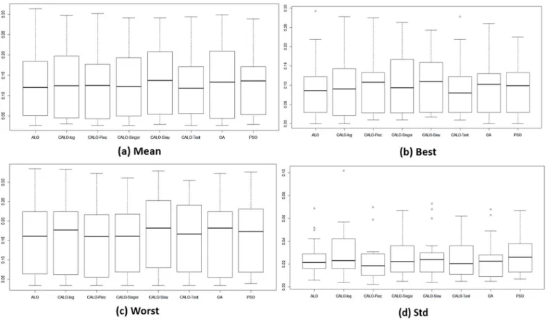
3.3 Analysis and discussion
Fig 4shows the average statistical mean fitness, best fitness, worst fitness, and the standard deviation for all the methods used and for all 18 datasets. The results for the biological datasets are presented in (Fig 5), and those for the other non-biological datasets are presented in (Fig 6). We can observe that ALO and CALO generally perform better than GA and PSO. The search method adopted in ALO is more explorative than the one used in GA and PSO because ALO performs a local search around a roulette wheel selected solution, and in this way, other areas (apart from the area around the current best) are explored. Because of the balanced con-trol of exploration and exploitation, the CALO algorithm outperforms the original ALO. The nonsystematic adaptation of exploration rate in the CALO allows the successive local and global searching and helps escaping from local minima that commonly exist in the search space. Thetentchaos map outperforms the other chaos maps, whereas thesinusoidalmap pro-vides the worst chaotic result.
To assess the stability of the stochastic algorithms and the stability to converge to the same optimal solution, we measure the statistical standard deviation (std) of the fitness values over different runs. The minimum for the std measure is obtained by CALO in almost all the data-sets, which reaffirms that CALO is more stable and can converge to the same optimal solution regardless of its stochastic and chaotic manner. In addition, we can see that thetentmap still performs better than the other maps in terms of its repeatability. The results for the classifica-tion accuracy presented inTable 3show that CALO obtains the best results for 11 of the data-sets, thus demonstrating the capability of CALO to find optimal feature combinations ensuring good test performance.
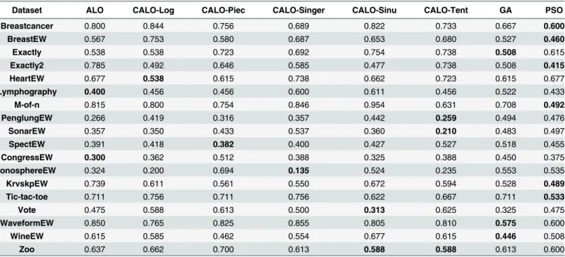
Table 4summarizes the results for the size of the selected feature subsets. We can see that CALO, while outperforming all the other methods in terms of classification performance, has comparable values with the other approaches for the number of features selected.
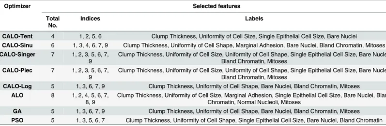
features. From the Breastcancer dataset, we can observe that CALO suggests that only four of the features are good enough to classify a tumor. As might be evident, it is particularly pre-ferred in biology and medicine to consider a small number of biomarkers for a disease because this involve fewer experiments, which may sometimes be difficult to perform and have side effects for the patient. For the Heart dataset, our method suggests that five of the data attributes will assure the same precision in performing the classification as if we consider all the features. Such tools could be of real help in the future as they will lead to fewer patient investigations and can lower the costs involved. Overall, while comparing CALO with GA and PSO, we observe that CALO almost always obtains better or very similar classification accuracy with a lower number of features selected. In the majority of the tests performed, on average, approxi-mately 75% of the features selected by CALO are in common with the features selected by GA or PSO, but in most of the cases, the set of features selected by CALO is included in the set of features selected by GA and PSO.
F-score values are given inTable 7, where we can again observe that CALO using thetent map obtains the best results overall. Additionally, note that the worst performing map is the sinusoidalmap.
Limitations. The main limitation of the methodology proposed in this paper is the non-exact repeatability of the optimization results. We observed that at different applications of the algorithm, the subset of features selected might differ. Although the resulting solutions are all good solutions, it may be confusing for the user to determine which subset to consider. The proposed algorithm works on the wrapper-based feature selection approach using the KNN Fig 4. The fitness values obtained from different methods for all 18 datasets.
Fig 5. The fitness values obtained from different methods for biological datasets.
doi:10.1371/journal.pone.0150652.g005
Fig 6. The fitness values obtained from different methods for non-biological datasets.
classifier as a simple one. The running time may increase when switching to another classifier, such as support vector machine (SVM) or random forest (RF). Therefore, switching to a differ-ent classifier should be carefully handled, particularly if the algorithm is adopted in real-time applications.
Table 3. Average classification accuracy of 20 independent runs for GA, PSO, ALO, and 5 different chaos maps of CALO.
Dataset ALO CALO-Log CALO-Piec CALO-Singer CALO-Sinu CALO-Tent GA PSO
Breastcancer 0.954 0.955 0.955 0.950 0.957 0.951 0.955 0.951
BreastEW 0.943 0.943 0.946 0.949 0.948 0.952 0.946 0.942
Exactly 0.660 0.675 0.655 0.671 0.681 0.661 0.659 0.671
Exactly2 0.741 0.737 0.747 0.730 0.761 0.736 0.728 0.737
HeartEW 0.824 0.813 0.813 0.811 0.822 0.820 0.802 0.824
Lymphography 0.744 0.772 0.732 0.728 0.720 0.724 0.744 0.692
M-of-n 0.875 0.891 0.882 0.880 0.851 0.930 0.867 0.841
PenglungEW 0.658 0.659 0.625 0.644 0.603 0.632 0.676 0.627
SonarEW 0.714 0.723 0.680 0.734 0.697 0.717 0.723 0.737
SpectEW 0.787 0.784 0.780 0.778 0.778 0.787 0.782 0.800
CongressEW 0.946 0.941 0.942 0.950 0.942 0.932 0.938 0.960
IonosphereEW 0.848 0.819 0.838 0.853 0.836 0.843 0.824 0.815
KrvskpEW 0.938 0.948 0.953 0.953 0.941 0.930 0.950 0.946
Tic-tac-toe 0.766 0.737 0.739 0.754 0.725 0.732 0.739 0.722
Vote 0.914 0.928 0.922 0.920 0.918 0.882 0.914 0.898
WaveformEW 0.769 0.765 0.767 0.766 0.764 0.762 0.766 0.757
WineEW 0.937 0.930 0.950 0.950 0.953 0.957 0.947 0.923
Zoo 0.836 0.798 0.805 0.854 0.846 0.860 0.824 0.805
doi:10.1371/journal.pone.0150652.t003
Table 4. Average selection size of 20 independent runs for GA, PSO, ALO, and 5 different chaos maps of CALO.
Dataset ALO CALO-Log CALO-Piec CALO-Singer CALO-Sinu CALO-Tent GA PSO
Breastcancer 0.800 0.844 0.756 0.689 0.822 0.733 0.667 0.600
BreastEW 0.567 0.753 0.580 0.687 0.653 0.680 0.527 0.460
Exactly 0.538 0.538 0.723 0.692 0.754 0.738 0.508 0.615
Exactly2 0.785 0.492 0.646 0.585 0.477 0.738 0.508 0.415
HeartEW 0.677 0.538 0.615 0.738 0.662 0.723 0.615 0.677
Lymphography 0.400 0.456 0.456 0.600 0.611 0.456 0.522 0.433
M-of-n 0.815 0.800 0.754 0.846 0.954 0.631 0.708 0.492
PenglungEW 0.266 0.419 0.316 0.357 0.442 0.259 0.494 0.476
SonarEW 0.357 0.350 0.433 0.537 0.360 0.210 0.483 0.497
SpectEW 0.391 0.418 0.382 0.400 0.427 0.527 0.518 0.455
CongressEW 0.300 0.362 0.512 0.388 0.325 0.388 0.450 0.375
IonosphereEW 0.324 0.200 0.694 0.135 0.524 0.235 0.553 0.535
KrvskpEW 0.739 0.611 0.561 0.550 0.672 0.594 0.528 0.489
Tic-tac-toe 0.711 0.756 0.711 0.756 0.622 0.667 0.711 0.533
Vote 0.475 0.588 0.613 0.500 0.313 0.625 0.325 0.475
WaveformEW 0.850 0.765 0.825 0.855 0.805 0.810 0.575 0.600
WineEW 0.615 0.585 0.462 0.554 0.677 0.615 0.446 0.508
Zoo 0.637 0.662 0.700 0.613 0.588 0.588 0.613 0.600
4 Conclusions
In this paper, we address the feature selection problem by developing a chaos-based version of a recently proposed meta-heuristic algorithm, namely, antlion optimization (ALO). A parame-ter whose setting is crucial for the algorithm performance is adapted using chaos principles. The proposed chaotic antlion optimization (CALO) is applied to a common challenging opti-mization problem: feature selection in the wrapper mode. The feature selection is formulated as a multi-objective optimization task with a fitness function reflecting the classification perfor-mance and the reduction in the number of features. The proposed system is evaluated using 18 different datasets against a number of evaluation criteria. We developed this method with par-ticular interest in datasets generated in biology, as these data typically have a large number of attributes and a low number of instances. CALO proves to be more efficient compared to ALO, PSO, and GA regarding the quality of the features selected. CALO is able to converge to the Table 5. An example of the feature selection size (reduction) for each optimization algorithm using theBreastcancerdataset.
Optimizer Selected features
Total No.
Indices Labels
CALO-Tent 4 1, 2, 5, 6 Clump Thickness, Uniformity of Cell Size, Single Epithelial Cell Size, Bare Nuclei
CALO-Sinu 6 1, 3, 4, 6, 7, 9 Clump Thickness, Uniformity of Cell Shape, Marginal Adhesion, Bare Nuclei, Bland Chromatin, Mitoses CALO-Singer 7 1, 2, 3, 5, 6, 7,
9
Clump Thickness, Uniformity of Cell Size, Uniformity of Cell Shape, Single Epithelial Cell Size, Bare Nuclei, Bland Chromatin, Mitoses
CALO-Piec 7 1, 2, 3, 5, 6, 7, 9
Clump Thickness, Uniformity of Cell Size, Uniformity of Cell Shape, Single Epithelial Cell Size, Bare Nuclei, Bland Chromatin, Mitoses
CALO-Log 5 1, 3, 6, 7, 9 Clump Thickness, Uniformity of Cell Shape, Bare Nuclei, Bland Chromatin, Mitoses ALO 8 1, 2, 4, 5, 6, 7,
8, 9
Clump Thickness, Uniformity of Cell Size, Marginal Adhesion, Single Epithelial Cell Size, Bare Nuclei, Bland Chromatin, Normal Nucleoli, Mitoses
GA 5 1, 3, 6, 7, 9 Clump Thickness, Uniformity of Cell Shape, Bare Nuclei, Bland Chromatin, Mitoses PSO 5 1, 3, 5, 6, 7 Clump Thickness, Uniformity of Cell Shape, Single Epithelial Cell Size, Bare Nuclei, Bland Chromatin
doi:10.1371/journal.pone.0150652.t005
Table 6. An example of the feature selection size (reduction) for each optimization algorithm using theHeartEWdataset.
Optimizer Selected features
Total No.
Indices Labels
CALO-Tent 5 3, 9, 10, 11, 12 chest pain type, exercise-induced angina, oldpeak, slope of the peak exercise ST segment, number of major vessels
CALO-Sinu 6 1, 3, 7, 9, 12, 13 age, chest pain type, resting electrocardiographic, exercise-induced angina, number of major vessels, defect type
CALO-Singer 8 1, 3, 4, 7, 8, 11, 12, 13
age, chest pain type, resting blood pressure, resting electrocardiographic, maximum heart rate, slope of the peak exercise ST segment, number of major vessels, defect type
CALO-Piec 8 1, 2, 3, 6, 8, 10, 11, 12
age, sex, chest pain type, fasting blood sugar, maximum heart rate, oldpeak, slope of the peak exercise ST segment, number of major vessels
CALO-Log 6 1, 2, 3, 7, 12, 13 age, sex, chest pain type, resting electrocardiographic, number of major vessels, defect type
ALO 6 2, 3, 5, 11, 12,
13
sex, chest pain type, serum cholesterol, slope of the peak exercise ST segment, number of major vessels, defect type
GA 7 3, 5, 8, 9, 10, 11, 12
chest pain type, serum cholesterol, maximum heart rate, exercise-induced angina, oldpeak, slope of the peak exercise ST segment, number of major vessels
PSO 8 1, 2, 3, 6, 7, 10, 12, 13
age, sex, chest pain type, fasting blood sugar, resting electrocardiographic, oldpeak, number of major vessels, defect type
same optimal solution for a higher number of applications compared to ALO, PSO, and GA, regardless of the stochastic searching and the chaotic adaptation. The performance of CALO is better than that of the other methods over the test data considered.
Acknowledgments
This work was partially supported by the IPROCOM Marie Curie initial training network, funded through the People Programme (Marie Curie Actions) of the European Union’s Sev-enth Framework Programme FP7/2007-2013/ under REA grants agreement No. 316555, and by the Romanian National Authority for Scientific Research, CNDI-UEFISCDI, project num-ber PN-II-PT-PCCA-2011-3.2-0917.
Author Contributions
Conceived and designed the experiments: EE HMZ. Performed the experiments: EE. Analyzed the data: HMZ. Contributed reagents/materials/analysis tools: HMZ CG. Wrote the paper: HMZ EE CG.
References
1. Chuang LY, Tsai SW, Yang CH. Improved binary particle swarm optimization using catfish effect for feature selection. Expert Systems with Applications. 2011; 38(10):12699–12707.
2. Dash M, Liu H. Feature selection for Classification. Intelligent Data Analysis. 1997; 1(3):131–156. doi: 10.1016/S1088-467X(97)00008-5
3. Huang CL. ACO-based hybrid classification system with feature subset selection and model parame-ters optimization. Neurocomputing. 2009; 73(1–3):438–448. doi:10.1016/j.neucom.2009.07.014 4. Duda RO, Hart PE, Stork DG. Pattern Classification. 2nd ed. Wiley-Interscience; 2000.
5. Chen Y, Miao D, R W. A rough set approach to feature selection based on ant colony optimization. Pat-tern Recognition Letters. 2010; 31(3):226–233. doi:10.1016/j.patrec.2009.10.013
Table 7. Average f-score of 20 independent runs for GA, PSO, ALO, and 5 different chaos maps of CALO.
Dataset ALO CALO-Log CALO-Piec CALO-Singer CALO-Sinu CALO-Tent GA PSO
Breastcancer 9.159 10.084 8.780 8.251 9.661 8.417 8.155 7.454
BreastEW 7.855 9.552 7.792 9.085 8.349 9.625 7.382 6.872
Exactly 0.017 0.016 0.022 0.023 0.024 0.025 0.018 0.021
Exactly2 0.025 0.014 0.020 0.018 0.014 0.023 0.015 0.015
HeartEW 1.408 1.241 1.301 1.410 1.356 1.453 1.254 1.370
Lymphography 3.104 3.203 5.110 4.633 4.436 2.506 5.390 4.084
M-of-n 0.403 0.403 0.403 0.404 0.404 0.401 0.389 0.323
PenglungEW 66.689 103.142 81.710 87.756 110.113 62.330 120.123 118.180
SonarEW 0.900 0.933 1.171 1.362 0.914 0.614 1.343 1.335
SpectEW 0.482 0.512 0.492 0.474 0.515 0.634 0.616 0.525
CongressEW 2.628 3.043 4.164 3.322 3.171 3.096 3.625 3.118
IonosphereEW 1.077 0.850 1.809 0.771 1.620 1.023 1.585 1.399
KrvskpEW 0.852 0.796 0.781 0.753 0.794 0.773 0.769 0.744
Tic-tac-toe 0.050 0.055 0.054 0.053 0.047 0.050 0.051 0.048
Vote 3.337 3.831 4.047 3.353 2.480 3.647 2.219 3.186
WaveformEW 6.178 5.903 6.110 6.314 5.823 5.875 5.485 5.241
WineEW 7.742 7.332 6.392 7.217 8.567 8.648 6.126 6.268
Zoo 299.533 226.958 288.376 267.946 260.639 265.226 244.569 298.357
6. Kohavi R, John GH. Wrappers for feature subset selection. Artificial Intelligence. 1997; 97(1):273–324. doi:10.1016/S0004-3702(97)00043-X
7. Xue B, Zhang M, Browne WN. Particle swarm optimisation for feature selection in classification: Novel initialisation and updating mechanisms. Applied Soft Computing. 2014;18:261–276. doi:10.1016/j. asoc.2013.09.018
8. Guyon I, Elisseeff A. An introduction to variable and attribute selection. Machine Learning Research. 2003; 3:1157–1182.
9. Whitney A. A direct method of nonparametric measurement selection. IEEE Transactions on Comput-ers. 1971; C-20(9):1100–1103. doi:10.1109/T-C.1971.223410
10. Marill T, Green D. On the effectiveness of receptors in recognition systems. IEEE Transactions on Infor-mation Theory. 1963; 9(1):11–17. doi:10.1109/TIT.1963.1057810
11. Xue B, Zhang M, Browne WN. Particle swarm optimization for feature selection in classification: a multi-objective approach. IEEE transactions on cybernetics. 2013; 43(6):1656–1671. doi:10.1109/TSMCB. 2012.2227469PMID:24273143
12. Shoghian S, Kouzehgar M. A Comparison among Wolf Pack Search and Four other Optimization Algo-rithms. Computer, Electrical, Automation, Control and Information Engineering. 2012; 6(12):1619– 1624.
13. Eiben AE, Raue PE, Ruttkay Z. Genetic algorithms with multi-parent recombination. In: Parallel Prob-lem Solving from Nature—PPSN III, International Conference on Evolutionary Computation. Springer; 1994. p. 78–87.
14. Kennedy J, Eberhart R. Particle swarm optimization. IEEE International Conference on Neural Net-works. 1995; 4:1942–1948.
15. Holland JH. Adaptation in natural and artificial systems. Cambridge, MA, USA: MIT Press; 1992. 16. Eberhart R, Kennedy J. A New Optimizer Using Particle Swarm Theory. In: International Symposium
on Micro Machine and Human Science. IEEE; 1995. p. 39–43.
17. Mirjalili S. The Ant Lion Optimizer. Advances in Engineering Software. 2015; 83:80–98. doi:10.1016/j. advengsoft.2015.01.010
18. Chen H, Jiang W, Li C, Li R. A Heuristic Feature Selection Approach for Text Categorization by Using Chaos Optimization and Genetic Algorithm. Mathematical Problems in Engineering. 2013; 2013:1–6. 19. Chakraborty B. Genetic algorithm with fuzzy fitness function for feature selection. In: International
Sym-posium on Industrial Electronics. IEEE; 2002. p.315–319.
20. Chakraborty B. Feature subset selection by particle swarm optimization with fuzzy fitness function. In: Third International Conference on Intelligent System and Knowledge Engineering. IEEE; 2008. p. 1038–1042.
21. Neshatian K, Zhang M. Genetic programming for feature subset ranking in binary classification prob-lems. In: Genetic Programming. Berlin: Springer; 2002. p. 121–132.
22. Gao HH, Yang HH, Y WX. Ant colony optimization based network intrusion feature selection and detec-tion. In: International Conference on Machine Learning and Cybernetics. IEEE; 2005. p. 3871–3875. 23. Ming H. A rough set based hybrid method to feature selection. In: International Symposium on
Knowl-edge Acquisition and Modeling. IEEE; 2008. p. 585–588.
24. Chuanwen J, Bompard E. A hybrid method of chaotic particle swarm optimization and linear interior for reactive power optimisation. Mathematics and Computers in Simulation. 2005; 68(1):57–65. doi:10. 1016/j.matcom.2004.10.003
25. Kim H, Howland P, Park H. Dimension reduction in text classification with support vector machines. Journal of Machine Learning Research. 2005; 6:37–53.
26. Oh IS, Lee JS, Moon BR. Hybrid genetic algorithms for feature selection. IEEE Transactions on Pattern Analysis and Machine Intelligence. 2004; 26(11):1424–1437. doi:10.1109/TPAMI.2004.105PMID: 15521491
27. Landassuri-Moreno V, Marcial-Romero JR, Montes-Venegas A, Ramos MA. Chaotic Time Series Pre-diction with Feature Selection Evolution. In: Conference in Electronics, Robotics and Automotive Mechanics. IEEE; 2011. p. 71–76.
28. Gholipour A, Araabi BN, Lucas C. Predicting Chaotic Time Series Using Neural and Neurofuzzy Mod-els: A Comparative Study. Neural Processing Letters. 2006; 24(3):217–239. doi: 10.1007/s11063-006-9021-x
29. Vohra R, Patel B. An Efficient Chaos-Based Optimization Algorithm Approach for Cryptography. Com-munication Network Security. 2012; 1(4):75–79.
31. Raouf OA, Baset MA, henawy IE. An Improved Chaotic Bat Algorithm for Solving Integer Programming Problems. Modern Education and Computer Science. 2014; 6(8):18–24. doi:10.5815/ijmecs.2014.08. 03
32. Aguirregabiria JM. Robust chaos with variable Lyapunov exponent in smooth one-dimensional maps. Chaos Solitons & Fractals. 2014; 42(4):2531–2539. doi:10.1016/j.chaos.2009.03.196
33. Saremi S, Mirjalili S, Lewis A. Biogeography-based optimisation with chaos. Neural Computing and Applications. 2014; 25(5):1077–1097. doi:10.1007/s00521-014-1597-x
34. Yang XS. Nature-Inspired, Metaheuristic Algorithms. 2nd ed. United Kingdom: Luniver Press; 2010. 35. Vieira SM, Sousa JMC, Runkler TA. Two cooperative ant colonies for feature selection using fuzzy
models. Expert Systems with Applications. 2010; 37(4):2714–2723. doi:10.1016/j.eswa.2009.08.026 36. Bache K, Lichman M. UCI Machine Learning Repository. type. 2013 [cited 2016 Jan 15];Available from:
http://archive.ics.uci.edu/ml.