SRef-ID: 1684-9981/nhess/2004-4-407
© European Geosciences Union 2004
and Earth
System Sciences
Probabilistic seismic hazard maps from seismicity patterns analysis:
the Iberian Peninsula case
A. Jim´enez1, 2, A. M. Posadas1, 2, 3, T. Hirata4, and J. M. Garc´ıa1, 2 1Department of Applied Physics, University of Almeria, Spain
2Andalusian Institute of Geophysics and Seismic Disasters Prevention, Spain 3‘Henri Poincar´e’ Chair of Complex Systems, University of La Havana, Cuba 4Department Human and Artificial Intelligent Systems, Fukui University, Japan
Received: 30 September 2003 – Revised: 5 April 2004 – Accepted: 1 June 2004 – Published: 10 June 2004
Abstract.
Earthquake prediction is a main topic in Seismology. Here, the goal is to know the correlation between the seis-micity at a certain place at a given time with the seisseis-micity at the same place, but at a following interval of time. There are no ways for exact predictions, but one can wonder about the causality relations between the seismic characteristics at a given time interval and another in a region. In this paper, a new approach to this kind of studies is presented. Tools which include cellular automata theory and Shannon’s en-tropy are used. First, the catalogue is divided into time in-tervals, and the region into cells. The activity or inactivity of each cell at a certain time is described using an energy crite-rion; thus a pattern which evolves over time is given. The aim is to find the rules of the stochastic cellular automaton which best fits the evolution of the pattern. The neighborhood uti-lized is the cross template (CT). A grid search is made to choose the best model, being the mutual information between the different times the function to be maximized. This func-tion depends on the size of the cellsβon and the interval of timeτ which is considered for studying the activity of a cell. With theseβ andτ, a set of probabilities which character-izes the evolution rules is calculated, giving a probabilistic approach to the spatiotemporal evolution of the region. The sample catalogue for the Iberian Peninsula covers since 1970 till 2001. The results point out that the seismic activity must be deduced not only from the past activity at the same region but also from its surrounding activity. The time and spatial highest interaction for the catalogue used are of around 3.3 years and 290×165 km2, respectively; if a cell is inactive, it will continue inactive with a high probability; an active cell has around the 60% probability of continuing active in the fu-ture. The Probabilistic Seismic Hazard Map obtained marks the main seismic active areas (northwestern Africa) were the real seismicity has been occurred after the date of the data set studied. Also, the Hurst exponent has been studied. The
Correspondence to:A. Jim´enez
value calculated is 0.48±0.02, which means that the process is inherently unpredictable. This result can be related to the incapacity of the cellular automaton obtained of predicting sudden changes.
1 Introduction
Perhaps, a first true physical understanding on prediction was advanced by Darwin (1913): “the foreshocks ’must mark out’ the place of next large event”. Some years later (1964), C. F. Richter said that ”Claims to predict usually come from cranks, publicity seekers, or people who pretend to foresee the future in general”. Although earthquakes can not be pre-dicted systematically, some scientific successful predictions have been made (Sykes and Nishenko, 1984; Scholz, 1985; Nishenko, 1989; Nishenko et al., 1996; Wyss and Burford, 1985; Purcaru, 1996; Kossobokov et al., 1997). Other stud-ies attempt to determine the characteristics of the next earth-quake in a region. For example, Varnes and Bufe (1996) and Torcal et al. (1999) show how the time periods of the next event can be determined in a seismic series by using geostatistical methods; Agostinelli and Rotondi (2003) used Bayesian belief networks to analyze the stochastic depen-dence between inter-event time and size of earthquakes; Ka-gan and Jackson (2000) made use of statistical models for short time prediction.
it is based on the ideas contained in the Theory of the Infor-mation described (for the first time) by Shannon (1948) and Shannon and Weaver (1949). This formalism was used by Shaw (1984) to study the temporal series produced by a drop of water that falls from a faucet not properly turned off. He established an alternative way to deal with complex problems by using recurrence plots in the phase space. The behavior and evolution of a system in which a series of states is known, states occurred at T1, T2, . . . , Tn, can be characterized by a
recurrence map; that is, by representing the state at Tiin the
x-axis, and the one at Ti+1in the y-axis, and the process goes on until the adequate dimension is obtained. Shaw used these plots and the concept of information based on Shannon’s en-tropy in order to study the evolution of the system, the knowl-edge of the future states from the present and the past states. A spatiotemporal occurrence model of earthquakes based on the information theory and cellular automata was presented by Posadas et al. (2000) and by Posadas et al. (2002); in the present paper their methodology is used to develop a map where the level of the future seismic activity is predicted and we assign a probabilistic value to such a level. We call this kind of representation a Probabilistic Seismic Hazard Map. In this paper the method is discussed by means of several tests, which show that the future activity of the different parts of a region is better described, in terms of the automata cellu-lar proposed, by taking into account not only their activity but also their neighboring activities than by supposing that the activity is propagated from a place to its neighboring sites. This kind of discussions is interesting, because in finite, real fault systems – such as the authors study – the interaction plays the crucial role in governing the seismicity dynamics.
2 Information theory
It has long been understood that physics and the notion of in-formation are intimately related. In a very real sense, the dif-ferential equations of physics are simply algorithms for pro-cessing the information contained in the initial conditions. Data obtained by experiment and observation either are, or contain information forming the basis of our understanding of nature (Grandy, 1997). But the concept of information is too broad to be embraced completely by a single defini-tion. However, for any probability distribution, a quantity called the entropy can be calculated, which has many prop-erties that agree with the intuitive notion of what a measure of information should be. The entropyH (X)of a discrete random variableX, withX={x1, x2, . . . , xN}is defined by:
H (X)=−X
x∈X
p(x)logp(x), (1)
the Kullback-Leibler’s distanceD(p||p′), also called relative entropy, can be used; it represents the difference between two probability distribution functions,pandp′, of the same vari-able (Cover and Thomas, 1991):
D(p||p′)=Xplog2
p
p′. (2)
The general dependence between two variablesX andY is measured by the mutual informationµI, which is defined as
the relative entropy between the joint probabilityp(x, y)and the marginal probabilitiesp(x)andp(y)(Fraser and Swin-ney, 1986):
µI(X;Y )= n X
i=1 m X
j=1
p(xi, yj)log2
p(xi, yj)
p(xi)p(yj)
. (3)
IfXrepresents the past states andY the future ones, Eq. (3) gives an estimation of the dependence between these vari-ables through the time. Note that when X and Y are in-dependent,p(x, y)=p(x) p(y)(definition of independence),
µI(X;Y )=0. This makes sense: if they are independent
ran-dom variables,Y will tell nothing aboutX.
3 The model
Cellular automata are simple mathematical idealizations of natural systems. They consist of a lattice of discrete identical sites, each site taking on a finite set of, say, integer values. The values of the sites evolve in discrete time steps accord-ing to rules that specify the value of each site in terms of the values of neighboring sites. Cellular automata may thus be considered as discrete idealizations of the partial differential equations often used to describe natural systems (Wolfram, 1983). They have been used in seismology for modeling the earthquake rupture process (Bak and Tang, 1989), or for modeling the subduction phenomenon (Leduc, 1997), for ex-ample. On the other hand, the concept of entropy has been used as an indicator in earthquake structure or physics with passage of time, where mutual information provides an infor-mational content of this structure (Purcaru, 1973; Nicholson et al., 2000; Sotolongo and Posadas, 2004). Both cellular automata and information theory will be used in this paper to establish some models for the dynamical characteristics of the seismic activity in a probabilistic way.
t
t+
τ
Fig. 1.Temporal evolution of the patterns.
Mode I
Mode II
Fig. 2.The two propagation modes.
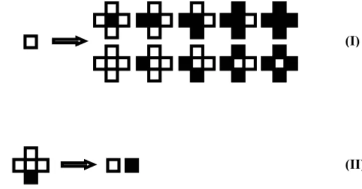
dimension (longitude or latitude). The accumulated energy of the events at a time intervalτ determines whether the cell is active or inactive. If this energy is greater than or equal to the average of the whole region, the cell is considered active. It is important to point out that this activation criterion is a relative one. The activity or inactivity of a cell depends on the averaged energy released in the whole region, so that an active cell is an area where the probability of seismic activity predicted is higher than the average. Other threshold activ-ity criteria could be tested, but this is not the purpose of the present paper. The goal is to compare two ways for finding the transition rules that give the patterns at a timet+τ tak-ing into account the information contained at timet, (Fig. 1 shows a hypothetical pattern series) and to chose the best one for a further generalization and improvement of the method. A simple method based on the mutual information is pre-sented to establish some models of propagation of the seis-mic activity in term of probabilities. The simplest cellular au-tomata model uses a template (Hirata and Imoto, 1997) in the form of a cross (cross template model or CT model). With this template, the activity dynamics can be looked at from two points of view: one can think of a propagation model where an active cell transmits its activity to its nearest neigh-borhood with different probabilities, or, on the contrary, to obtain the activity of a cell from its neighborhood at a previ-ous time (Fig. 2).
The mutual information contained can be calculated in both cases with this equation, which depends on the time and space intervals:
µI= 1 X
i=0 1 X
j=0 5 X
k=0
p(i;j, k)log2 p(i;j, k)
p(i)p(j, k) (4)
being p(i;j, k) the joint probability of states, and
p(i)p(j, k) a distribution of independent states; (i)stands
(I)
(II)
Fig. 3.Number of final states for each mode.
for the central cell and(j, k)for the central and its nearest neighboring cells (Posadas et al., 2002).
The time delayed mutual information was suggested by Fraser and Swinney (1986) as a tool to determine a reason-able delay. Unlike the autocorrelation function, the mutual information also takes into account nonlinear correlations. Maximizing Eq. (4), which depends on the template cho-sen (CT model), on the time intervalτ, and on N, the best configuration, which will give the maximum dependence be-tween consecutive patterns, can be calculated. This is done by searching in a grid with two variables: the interval of time
τ, obtained by dividing the whole time considered into a cer-tain number of steps, and the size of the cellsβ, obtained by dividing the whole area byN×N. With this optimum con-figuration (τ,β), determined with the information theory, the dependence between states has to be modeled.
For the Mode I, the model developed by Posadas et al. (2000) can be used; it is necessary to find the three prob-abilities, P1, P2 andP3, which determine the seismic pat-tern evolution, where the Kullback-Leibler’s distance is used again. The objective is to minimize this distance between the joint probability of consecutive states and the distribu-tion given by the productp′=p(i)p(j;k/ i), beingp(i)the initial state probability andp(j;k/ i)the conditional proba-bility, given by the propagation model (Posadas et al., 2000, 2002):
D(p||p′)=
1 X
i=0 1 X
j=0 5 X
k=0
p(i;j, k)log2 p(i;j, k)
p(i)p(j;k/ i). (5)
The optimization is made with a simple genetic algorithm, whose search parameters are P1, P2 and P3. Also, the seismic pattern evolution can be modeled by means of his-tograms of occurrences, and assigning the probability of find-ing a final state given an initial one. In this case, as shown in Fig. 3, it is easier if there are fewer final states; and that happens when the neighborhood determines the future state of the central cell (Mode II).
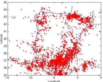
Fig. 4.Epicentral distribution of the analyzed events (from the Na-tional Geographic Institute (IGN), Spain).
there will be only two possibilities in the future (active or inactive), and not ten, which is more difficult to predict.
These two Modes are compared by calculating the opti-mum values forτ andβ, and by obtaining the transition rules for each Mode. For Mode I, the model is determined by the
P1,P2 andP3probabilities, and for Mode II, the model is obtained from the histograms. To decide which Mode is bet-ter, some tests have been carried out, explained in the next section.
4 Simulation and tests
The simulations intend to reproduce the sequence of pat-terns obtained, by using the past information and the rules given for each model. Afterwards, the results are checked by comparing the simulated patterns against the real ones. To do this, the tests used are the correlation function (Vicsek, 1992), that gives some information about the size of the clus-ters, and the Hamming distance, that tells how many times one has failed in predicting a cell. The Hamming distance is a common way to compare two bit patterns, and it is defined as the number of bits different in the two patterns (Ryan and Frater, 2002). More generally, if two ordered lists of items are compared, the Hamming distance is the number of items that do not identically agree. This distance is applicable to encoded information, and is a particularly simple metric of comparison.
Simulations are made as follows: supposing that the opti-mum time interval is given by seven steps, the starting point is the first real pattern corresponding toτ. Following the rules given byP1,P2andP3(Mode I), or, otherwise, by us-ing the histograms (Mode II), a simulation for the time 2τ is reproduced. The simulated seismic patterns have to be cal-culated to compare them with real data. From the transition rules the probability of activation for each cell is calculated,
6 8 10 12 14 16 18 20 22 24 2 5 8
bin
0-0.1
(bits)
Fig. 5.Mode I. Mutual information in function of steps and bins.
6 8 10 12 14 16 18 20 22 24 2 5 8 11 14 17 20
bin
step 0.2-0.3
0.1-0.2 0-0.1
(bits)
Fig. 6.Mode II. Mutual information in function of steps and bins.
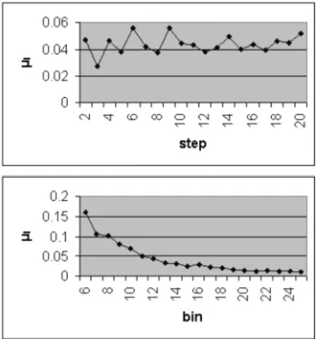
Fig. 7.Mode I. Averaged mutual information along the step and bin axis.
5 Application to the Iberian Peninsula seismicity
5.1 Data
The analyzed area is the region between 35◦and 45◦ north latitude and between 15◦ west and 5◦ east longitude. The used catalogue is from the National Geographic Institute (Spain) and it contains all the seismic data in the Iberian Peninsula and northwestern Africa. Around 10 000 earth-quakes have been collected in the period 1970–2001 (Fig. 4). The depths of the earthquakes range from 0 to 146 km, and the magnitudes are between 2.0 and 6.5 (mb).
The Institute runs the National Seismic Network, with 42 stations, 35 of them of short period connected in real time with the Reception Centre of Seismic Data in Madrid. The average errors in the hypocentral localization at the X, Y and Z directions, are±5 km, ±5 km and ±10 km, respec-tively, for the data recorded until 1985, and±1 km,±1 km and±2 km for those acquired since 1985. The Gutenberg-Richter relationship is satisfied. This is a quality criterion, so that if this was not the case, the data could not be assumed as free of slant or abnormal seismicity (Gonz´alez, 2002). 5.2 Application and results
The mutual information values are similar for both modes. There is a maximum of 0.25–0.26 bits for steps = 6 and bins = 6, and other one of around 0.20 bits for steps = 9 and bins = 6 (Figs. 5 and 6). The averaged mutual information has a maximum at steps = 9 in both cases, and the maximum
Fig. 8. Mode II. Averaged mutual information along the step and bin axis.
t
t+
τ
t+2
τ
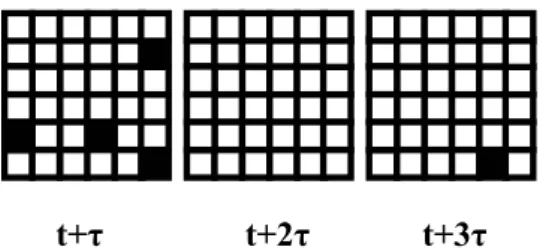
Fig. 9. Real patterns for 6×6 cells and 6 steps. (Active cells are drawn in black color, and inactive ones in white). Patterns corre-sponding to t+3τ, t+4τ, t+5τare the same as t+2τ.
obtained by averaging along the bin axis is always found at bins = 6 (Figs. 7 and 8).
The patterns evolution are modeled with both Modes (I and II) for these maxima (Figs. 9 to 14), and, afterwards, the results are compared to decide the best configuration in function of the success of the simulations found with each Mode.
The model, for the Mode I and the first maximum (6 bins, 6 steps), is determined by the following probabilities:
P1=0.4922,P2=0.1177 andP3=0.0265. With this model and after a time τ, there is a probability of 50% that the same cell will continue active, of around 12% that an active cell propagates its activity to the neighbors, and one of 3% that an inactive cell becomes active. For the second maximum (6 bins, 9 steps), the model is: P1=0.6274,P2=0.1499, and
be-Fig. 10. Simulated patterns for 6×6 cells and 6 steps (Mode I). Patterns corresponding to t+4τ, t+5τare the same as t+3τ.
t+
τ
t+2
τ
t+3
τ
Fig. 11. Simulated patterns for 6×6 cells and 6 steps (Mode II). Patterns corresponding to t+4τ, t+5τare the same as t+3τ.
tween patterns is this test. Taking into account that, the sec-ond configuration (6 bins, 9 steps) is chosen, because of its better accuracy; that is, the averaged number of simulated cells failed is smaller (for the first maximum is 1.6 bits, and for the second one is 1.125 bits, as shown in Figs. 13 and 14). The models for the Mode II are the histograms found in the data. Tables 1–2 show the transition probabilities for each maximum, appearing as rules of a stochastic cellular au-tomaton. There are some transitions that are not catalogued, because they were not found in the data (they are denoted as NC). Also, the tests made for the simulations are presented in Figs. 17 and 18. The averaged Hamming distance for the first minimum is 0.8, and for the second one is 0.75. As for Mode I, the second configuration is the best. Moreover, Mode II fits better than Mode I, either by comparing one to one the two maxima, or by taking into account both configurations. The Hamming distance is always lower, and the correlations functions are closer with Mode II. So, this is the schema pro-posed for this kind of analysis. And as a result of this study, the configuration selected for the data used corresponds to a grid of 6×6 cells and 9 intervals of time.
In Fig. 19, it can be seen that the main activity predicted (in the sense of having more activity than the average) is placed in the northwestern Africa. Since the highest mag-nitude releases have been occurred there, the seismic hazard must be higher in these places, in agreement with the results presented. The interesting contribution in this paper is the quantitative evaluation (in probabilistic terms) of the interac-tion between the different parts of the region, by providing the times and sizes that best fit the available data, so that a spatiotemporal characterization of the seismic behavior is made.
It is also interesting to know the averaged energy release necessary for the activation of each zone. For this catalogue
Fig. 12. Real patterns for 6×6 cells and 9 steps. Patterns corre-sponding from t+4τto t+8τare the same as t+3τ.
t+
τ
t+2
τ
t+3
τ
t+4
τ
Fig. 13. Simulated patterns for 6×6 cells and 9 steps (Mode I). Patterns corresponding from t+5τto t+8τare the same as t+4τ.
and the resulting bins and steps, the average needed in each step is around the correspondent to a magnitude equal to 5.5. This can be seen as a characteristic magnitude of the region analyzed. If the events of the Algerian zone and those of the north of Morocco are eliminated, and then this method is used, the resultant map might mark the main seismogenetic zones of the Iberian Peninsula. But, as explained, the objec-tive of the present study is the comparison between Mode I and II, and to establish a solid basis for other works. So the discussion will be leaved for future studies.
Following the analysis, as can be observed in Table 2, if a cell is inactive, it will continue inactive with a high probabil-ity; an active cell has around the 60% probability of continu-ing active in the future. Other important feature of the pattern evolution is that sudden changes are not well modeled. The predictions made by this model (Mode II) tend to repeat the latest patterns. An interesting analysis about this behavior is carried out by doing a diagram of cumulative seismic energy (Goltz, 1997). Figure 20 shows such a diagram for the data set analyzed, with the typical shape of a Devil’s staircase.
Lomnitz (1994) used this kind of plots to study the earth-quake cycles, and applied to them the Hurst method. He found that these processes have the behavior of the so-called “Joseph effect” (Mandelbrot and Wallis, 1968): quiet years tend to be followed by quiet years, and active years by ac-tive years. This corresponds to a Hurst exponent,H, greater than 1/2. However, Ogata and Abe (1991) obtained values ofH of about 0.5, with data from Japan and from the whole world. This means that successive steps are independent, and the best prediction is the last measured value.
t+
τ
t+2
τ
t+3
τ
t+4
τ
Fig. 14. Simulated patterns for 6×6 cells and 9 steps (Mode II). Patterns corresponding from t+5τto t+8τare the same as t+4τ.
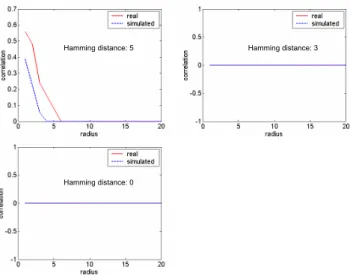
Hamming distance: 5 Hamming distance: 3
Hamming distance: 0
Fig. 15.Correlation functions and Hamming distances of the simu-lations for 6×6 cells and 6 steps (Mode I). After the 4t hstep there are no changes.
(1991), and the model obtained before reproduces this be-havior, namely, to repeat the latest patterns, and with inca-pacity to predict sudden changes. This would be imposed by the nature of the phenomenon, because of its inherent unpre-dictability.
6 Conclusions
A spatiotemporal characterization of the seismic dynamics can be made by maximizing the mutual information, which takes into account any kind of correlation. An energy crite-rion for the activation has been introduced, to give the ad-equate importance to the areas with less number of events, but with high magnitudes. A new point of view has been adopted, where a neighborhood determines the activation of its central cell at the future (Mode II). It could be interpreted as the risk of being activated, not only from its previous ac-tivity, but also from the activity of the nearest neighboring cells. This model gives rules for the transition probabilities between past and present states, whose simulations are bet-ter than those obtained by theP1,P2andP3model (Mode I). This means that the calculations have been simplified, and the generalization to other neighborhoods and dimensions is easier than with the old scheme.
Hamming distance: 2 Hamming distance: 4
Hamming distance: 3 Hamming distance: 0
Fig. 16.Correlation functions and Hamming distances of the simu-lations for 6×6 cells and 9 steps (Mode I). After the 4t hstep there are no changes.
Hamming distance: 3 Hamming distance: 1
Hamming distance: 0
Fig. 17.Correlation functions and Hamming distances of the simu-lations for 6×6 cells and 6 steps (Mode II). After the 4t hstep there are no changes.
simi-Hamming distance: 1 Hamming distance: 0
Fig. 18.Correlation functions and Hamming distances of the simu-lations for 6×6 cells and 9 steps (Mode II). After the 5t hstep there are no changes.
Fig. 19. Seismic hazard map of the Iberian Peninsula and north-western Africa. The color bar marks the activation probability of the zone.
lar seismic behavior. With large areas, an average of rules is made, to the detriment of having a good resolution or more success. A similar result was obtained by Lomnitz (1994), who showed that the Hurst analysis should not be applied to large complex regions, because the localized effects super-impose each other in such a way that statistics is destroyed. To avoid this, smaller areas should be studied; or the model should be complicated, by choosing a different template or neighborhood, with a higher number of cells.
Finally, it is remarkable the coincidence between the pre-diction made with this simple model (with a catalogue from 1970 to 2001) and the seismicity observed since 2001. Ex-cept for a few earthquakes, the main activity has been pro-duced in the north of Africa, near the predictions (http://neic. usgs.gov/neis/epic/epic.html). These results stimulate us to
Fig. 20. Cumulative seismic energy for the Iberian Peninsula and northwestern Africa.
Fig. 21. Hurst diagram for Iberian Peninsula and northwestern Africa in the period 1970–2001. N is the size of the time interval and R/S is the rescaled range (for calculation details, see Gimeno, 2000).
continue our research with this method, by testing other ac-tivation criteria (mainly, threshold criteria) and other neigh-borhoods.
Acknowledgements. The authors thank J. M. Marfil, whose com-ments and useful discussions at the various stages of this study led to an improvement of it, and G. Purcaru, for assisting in evaluating this paper and for his constructive critical remarks. This work was partially supported by the MCYT project REN2001-2418-C04-02/RIES, the MCYT project REN2002-04198-C02-REN2001-2418-C04-02/RIES, the MCYT project REN2004-CO3-02/RIES and the Research Group ”Geof´ısica Aplicada” RNM194 (Universidad de Almer´ıa, Espa˜na) belonging to the Junta de Andaluc´ıa.
Edited by: T. Glade
Table 1. Transition probabilities for 6×6 cells and 6 steps (Mode II). The first and the third columns give the initial and final states of the central cells, respectively (0 is inactive, and 1 is active). The second column represents the number of active neighboring cells.
Initial state Neighbors Final state Probability
0 0 0 1.00
0 0 1 0.00
0 1 0 0.96
0 1 1 0.04
0 2 0 0.80
0 2 1 0.20
0 3 0 1.00
0 3 1 0.00
0 4 0 NC
0 4 1 NC
1 0 0 0.50
1 0 1 0.50
1 1 0 0.50
1 1 1 0.50
1 2 0 0.75
1 2 1 0.25
1 3 0 NC
1 3 1 NC
1 4 0 NC
1 4 1 NC
Table 2. Transition probabilities for 6×6 cells and 9 steps (Mode II). The first and the third columns give the initial and final states of the central cells, respectively (0 is inactive, and 1 is active). The second column represents the number of active neighboring cells.
Initial state Neighbors Final state Probability
0 0 0 1.00
0 0 1 0.00
0 1 0 0.97
0 1 1 0.03
0 2 0 0.88
0 2 1 0.13
0 3 0 1.00
0 3 1 0.00
0 4 0 NC
0 4 1 NC
1 0 0 0.36
1 0 1 0.64
1 1 0 0.38
1 1 1 0.63
1 2 0 0.40
1 2 1 0.60
1 3 0 NC
1 3 1 NC
1 4 0 NC
1 4 1 NC
References
Agostinelli, C. and Rotondi, R.: Using Bayesian belief networks to analyze the stochastic dependence between inter-event time and size of earthquakes, J. Seism., 7, 281–299, 2003.
Bak, P. and Tang, C.: Earthquakes as a Self-Organized Critical Phe-nomenon, J. Goephys. Res., 94, 15 635–15 637, 1989.
Cover, T. and Thomas, J.: Elements of information theory, Wiley & Sons, New York, 1991.
Darwin, C.: The prevision of earthquakes, Gerlands Beitr. Geo-physik, 12, 9–15, 1913.
Fraser, A. and Swinney, H.: Independent coordinates for strange attractors from mutual information, Phys. Rev. A, 33, 2, 1134– 1140, 1986.
Gimeno, R.: An´alisis Ca´otico de Series Temporales Financieras de Alta Frecuencia. El Contrato de Futuro sobre el Bono Nocional a 10 a˜nos, Ph. D. Thesis, Universidad Pontificia de Comillas, Madrid, 2000.
Goltz, C.: Fractal and chaotic properties of earthquakes, Springer, Berlin, 1997.
Gonz´alez, J. L.: Caracterizaci´on entr´opica de la propagaci´on s´ısmica, Ph. D. Thesis, University of Almer´ıa, 2002.
Grandy, W. T., Jr: Resource letter ITP-1: Information Theory in Physics, Am. J. Phys., 65, 466–476, 1997.
Hirata, T. and Imoto, K.: A probabilistic cellular automaton ap-proach for a spatiotemporal seismic activity pattern, Zisin, 2, 49, 441–449, 1997.
Kagan, Y. Y. and Jackson, D. D.: Probabilistic forecasting of earth-quakes, Geophys. J. Int., 143, 438–453, 2000.
Kossobokov, V. G., Healy, J. H., and Dewey, J. W.: Testing an earth-quake prediction algorithm, Pure Appl. Geophys., 149 , 219–248, 1997.
Leduc, T.: One-dimensional discrete computer model of the sub-duction erosion phenomenon (plate tectonics process), In pro-ceedings of CESA’98, Simposium in Applied Mathematics and Optimization, 1997.
Lomnitz, C.: Fundamental of earthquake prediction, Wiley & Sons, New York, 1994.
Mandelbrot, B. B. and Wallis, J. R.: Noah, Joseph and the opera-tional hydrology, Water Resour. Res., 4, 5, 909–918, 1968. Nicholson, T., Sambridge, M., and Gudmundsson, O.: On entropy
and clustering in earthquake hypocenter distributions, Geophys. J. Int, 142, 37–51, 2000.
Nishenko, S. P.: Earthquake hazards and prediction, Encyclopedia of Solid Earth and Geophysics, edited by James, D. E., Van Nos-trand Reinhold, 260–268, 1989.
Nishenko, S. P., Bufe, C., Dewey, J., Varnes, D., Healy, J., Jacob, K., and Kossobokov, V.: 1996 Delarof Islands earthquake – a successful earthquake forecast/prediction? Eos (American Geo-physical Union Transactions), 77, 46, 456, 1996.
Ogata, Y. and Abe, K.: Some statistical features of the long-term variation of the global and regional seismicity, Int. Stat. Review, 59, 139–161, 1991.
Pe˜na, J., Vidal, F., Posadas, A. M., Morales, J., Alguacil, G., de Miguel, F., Ib´a˜nez, J., Romacho, M., and L´opez-Linares, A.: Space clustering properties of the Betic-Alboran earthquakes in the period 1962–1989, Tectonophysics, 221, 125–134, 1993. Posadas, A., Hirata, T., and Vidal, F.: Information theory to
charac-terize spatiotemporal patterns of seismicity in the Kanto region, Bull. Seism. Soc. Am., 92, 600–610, 2002.
applica-Ryan, M. J. and Frater, M. R.: Communications and information systems, Argos Press, Red Hill, Australia, 2002.
Shannon, C. E.: The mathematical theory of communication, The Bell System Technical Journal, 27, 379–423, 623–656, 1948. Shannon, C. E. and Weaver, W.: The mathematical theory of
com-munication, The Board of Trustees of the University of Illinois, University of Illinois Press, 1949.
Shaw, R.: The dripping faucet as a model chaotic system, The Sci-ence Frontier Express Series, Aerial Press, Santa Cruz, Califor-nia, 1984.
Scholz, C. H.: The Black Mountain asperity: seismic hazard of the southern San Francisco peninsula, California, Geophys. Res. Lett., 12, 717–719, 1985.
ity of occurrence of earthquakes belonging to a seismic series, Geophys. J. Int., 139, 703-725, 1999.
Varnes D. J. and Bufe, C. G.: The cyclic and fractal seismic series preceding an mb 4.8 earthquake on 1980 February 14 near the Virgin Islands, Geophys. J. Int., 139, 149–158, 1996.
Vicsek, T.: Fractal growth phenomena, World Scientific, London, 1992.
Wolfram, S.: Cellular automata, Los Alamos Science, 9, 2–21, 1983.