The multifractal structure of satellite sea surface temperature maps can be used to obtain global maps of streamlines

(1)

OSD

6, 129–151, 2009

The MF structure of SST trace streamlines

A. Turiel et al.

Title Page

Abstract Introduction

Conclusions References

Tables Figures

◭ ◮

Back Close

Full Screen / Esc

Printer-friendly Version

Interactive Discussion Ocean Sci. Discuss., 6, 129–151, 2009

www.ocean-sci-discuss.net/6/129/2009/

Ocean Science Discussions

Papers published inOcean Science Discussionsare under open-access review for the journalOcean Science

The multifractal structure of satellite sea

surface temperature maps can be used to

obtain global maps of streamlines

A. Turiel1, V. Nieves1, E. Garcia-Ladona1, J. Font1, M.-H. Rio2, and G. Larnicol2 1

Institut de Ci `encies del Mar, CSIC, Barcelona, Spain

2

CLS – Space Oceanography Division, Toulouse, France

Received: 18 November 2008 – Accepted: 8 December 2008 – Published: 22 January 2009 Correspondence to: A. Turiel ([email protected])

(2)

OSD

6, 129–151, 2009

A. Turiel et al.

Title Page

Tables Figures

◭ ◮

Back Close

Full Screen / Esc

Interactive Discussion Abstract

Nowadays Earth observation satellites provide information about many relevant vari-ables of the ocean-climate system, such as temperature, moisture, aerosols, etc. How-ever, to retrieve the velocity field, which is the most relevant dynamical variable, is still a technological challenge, specially in the case of oceans. New processing techniques,

5

emerged from the theory of turbulent flows, have come to assist us in this task. In this paper, we show that multifractal techniques applied to new Sea Surface Temperature satellite products opens the way to build maps of ocean currents with unprecedented accuracy. With the application of singularity analysis, we show that global ocean cir-culation patterns can be retrieved in a daily basis. We compare these results with

10

high-quality altimetry-derived geostrophic velocities, finding a quite good correspon-dence of the observed patterns both qualitatively and quantitatively. The implications of this findings from the perspective both of theory and of operational applications are discussed.

1 Introduction

15

Earth observation satellites provide an excellent platform for continuously monitoring the climatic evolution of our planet. Present remote sensors provide, on a rutinary basis and at global scales, a wide set of measured variables such as Sea Surface Temper-ature (SST), water vapor content in atmosphere, ocean surface chlorophyll concen-tration, aerosol concentration in air and a long etc. Atmospheric and ocean studies

20

have largely been benefited from it, although the characterization of ocean dynamics by means of satellite observations is however more elusive than that of atmosphere. First, because due to the highest optical extinction of ocean water, our satellite-based knowledge about the ocean is limited to a narrow layer close to surface, of a depth going from millimeters to a few meters. Second, because despite some recent

devel-25

(3)

OSD

6, 129–151, 2009

A. Turiel et al.

Title Page

Tables Figures

◭ ◮

Back Close

Full Screen / Esc

Interactive Discussion directly obtain a crucial dynamic variable as the ocean velocity field from satellites is

still a challenging task.

Velocities can be retrieved through the Sea Surface Height (SSH) measurements from radar altimetry. The SSH field is linked to the pressure field and then the geostrophic approximation may be used to derive the velocity field. As a result

quasi-5

synoptic maps can be build through the interpolation of several altimeters (Traon et al., 1998) and have been used to study the ocean variability at relatively large scales (Wun-sch and Stammer, 1998). Sampling limitations as well as the necessity to combine the signals of several altimeters limit the spatial and time resolutions and prevent altimetry maps to resolve part of the relevant oceanic processes (Pascual et al., 2006).

10

An alternative strategy to evaluate ocean surface velocities from satellite data is to process sequences of images of SST (Bowen et al., 2002) or other scalars (Crocker et al., 2007). These techniques are based on tracking ocean structures which have been generated by the flow and are still being dragged (advected) by it. This strategy leads to useful velocity fields, although the spatial and temporal resolutions are

rel-15

atively limited due to processing needs, and sometimes the field is not well resolved. However, satellite images of scalar variables can still be further exploited to gain insight about the dynamics, taking advantage of the turbulent structure of ocean flows.

When turbulence develops in a flow, a very complicated structure raises. In a tur-bulent flow, intermittency is revealed as dramatic changes of velocity and other

prop-20

erties as one moves across the fluid domain. As a consequence, shear is dominant over many areas; scalar parcels dragged by two different filaments rapidly separate from each other and so the flow is continuously creating new singularity fronts. By singularity we understand that the value of the local singularity exponent (a measure of the function regularity (Daubechies, 1992; Turiel and Parga, 2000)) decreases, what

25

(4)

OSD

6, 129–151, 2009

A. Turiel et al.

Title Page

Tables Figures

◭ ◮

Back Close

Full Screen / Esc

Interactive Discussion (Turiel et al., 2005b; Isern-Fontanet et al., 2007; Turiel et al., 2008a) some authors

have argued that extracting singularities from satellite images as SST maps serves to delineate flow streamlines. Expressed in other words, singularity exponents are advected by the flow, what is an appropriate assumption as far as the stirring by the horizontal advection is the main singularity-inducing effect. This hypothesis is

sup-5

ported by the facts that at the mesoscale ocean flows are practically bi-dimensional and dominated by geostrophic balance and both SST and Chlorophyll images exhibit a common turbulent signature (Nieves et al., 2007).

In this paper, we will prove for the first time that singularity exponents derived from microwave SST maps serve to trace streamlines of surface currents, and at the same

10

time we will validate a new generation of altimeter products. In Sect. 2 we will present the data to be used in this study. Then, in Sect. 3 the concept of singularity exponent field of a scalar map is introduced and discussed, and some examples are shown. We thus proceed to Sect. 4, where the streamlines derived from singularity analysis of SST maps are compared with altimetry-derived geostrophic currents. Finally, the

con-15

clusions are presented in Sect. 5. Technical details are presented in the Appendices.

2 Description of the data

Our main source of data for this study are Optimally Interpolated (OI) SST images from Microwave (MW) Radiometer SSTs. Microwave OI SST data are produced by Re-mote Sensing Systems and sponsored by National Oceanographic Partnership

Pro-20

gram (NOPP), the NASA Earth Science Physical Oceanography Program, and the NASA REASoN DISCOVER Project. Data are available through the following web site: http://www.remss.com.

As SST images contain irregularly spaced data (in time and space) due to orbital gaps or environmental conditions, an interpolation of the data onto a regularly

sam-25

(5)

OSD

6, 129–151, 2009

A. Turiel et al.

Title Page

Tables Figures

◭ ◮

Back Close

Full Screen / Esc

Interactive Discussion This is possible by blending TMI and AMSR-E SSTs, providing nearly complete global

coverage each day. Near real time OI SST products are created daily, even if no new observations exist. However, the product is 0.25×0.25 degree gridded, which is a coarse resolution in comparison with the standard infrared SSTs one. Process-ing details can be found in Reynolds and Smith (1994) and at the followProcess-ing website:

5

http://www.ssmi.com/sst/microwave oi sst browse.html.

The second source of data for this study are geostrophic surface currents computed at CLS in the framework of the SURCOUF project (Larnicol et al., 2006). Two types of currents maps are produced by SURCOUF. First, real time global maps of surface cur-rents, which are produced daily on a 1/3◦Mercator grid. Second, a reanalysis of these

10

currents exists for the period June 1999–January 2006. In this study, the SURCOUF daily delayed-time maps of absolute geostrophic surface currents are used for the pe-riod September 2002 to August 2003. This pepe-riod is particularly interesting since four altimetric satellites (Jason-1, ERS2/ENVISAT, TOPEX interleaved, GFO) were working together, allowing a much improved description of the ocean mesoscale (Pascual et al.,

15

2006).

SURCOUF currents are based on the use of the altimetric data distributed by AVISO (http://www.aviso.oceanobs.com) and processed through the following steps: First, the usual geophysical corrections were applied to the altimetric heights from the four satel-lites (apart from GFO, for which specific corrections were applied (Traon et al., 2003))

20

and Sea Level Anomalies were computed subtracting from the instantaneous altimet-ric heights a 7 year (1993–1999) mean profile. Specific processing was applied to TP interleaved and GFO to achieve consistency with the Jason-1 and ERS2-ENVISAT mis-sions (Traon et al., 2003; Traon and Dibarboure, 2004). Then the along-track anomalies from the four different missions were mapped into a global 1/3◦resolution Mercator grid

25

(6)

assump-OSD

6, 129–151, 2009

A. Turiel et al.

Title Page

Tables Figures

◭ ◮

Back Close

Full Screen / Esc

Interactive Discussion tion. In the equatorial band the quasi geostrophic approximation is applied (Lagerloef

et al., 1999).

3 Characterization of streamlines by singularity exponents

The first step in our work is to design stable, high-performance tools to perform sin-gularity analysis on real images, capable to assign an accurate value of sinsin-gularity

5

exponent at each point. The singularity exponent of a scalar at a given point is a scale-invariant, dimensionless measure of the degree of regularity or irregularity of the function at that point (see Isern-Fontanet et al., 2007, and Turiel et al., 2008a, for a full discussion of the concept). As furnished by the acquisition devices, images (prop-erly speaking, 2-D maps of a given variable) do not vary continuously on space but are

10

sampled on a discrete grid, and are also affected by several sources of error, noise and acquisition problems. Hence, singularity analysis must implement appropriate filtering and interpolation schemes (Daubechies, 1992; Arneodo et al., 1995).

In this paper, we have used the same strategy developed in Turiel and Parga (2000), which has been shown to attain good spatial and value accuracy in the determination of

15

singularity exponents in many contexts and in particular for the processing of satellite imagery (Turiel et al., 2005a,b; Isern-Fontanet et al., 2007; Nieves et al., 2007; Turiel et al., 2008a). We will denote the scalar under study byθ(x) (where θ can be SST, chlorophyll concentration, etc, andx denotes the point in the image plane). At each location x the singularity exponent h(x) can be obtained by processing the wavelet

20

projections (Daubechies, 1992; Mallat, 1999) of the modulus of the gradient ofθ, that we denote byT_Ψ[|∇θ|](x, r) and are defined as follows:

T_Ψ[|∇θ|](x, r) ≡

Z

dx′|∇θ|(x′)1 r2Ψ

x−x′ r

(1)

As shown in previous works (Turiel et al., 2005b; Isern-Fontanet et al., 2007; Nieves et al., 2007) the wavelet projection of gradients of SST and other scalars depend on

(7)

OSD

6, 129–151, 2009

A. Turiel et al.

Title Page

Tables Figures

◭ ◮

Back Close

Full Screen / Esc

Interactive Discussion the scale resolution parameterr as a power-law, characterized by the local singularity

exponenth(x) in the way: T_Ψ[|∇θ|](x, r)=α(x)rh(x) + o

rh(x) ₍₂₎

where the expression orh(x)

means a term which is negligible compared to rh(x)

whenrh(x)

goes to zero. Scalars submitted to turbulence present local power-law

scal-5

ing at each one of its points as the one expressed by Eq. (2). This is connected to the Microcanonical Multifractal Formalism (Turiel et al., 2008b): Eq. (2) implies that θ is multifractal (i.e. a composite of multiple fractal interfaces) and at the same time allows to explicitly separate each fractal interface from a given signalθ(x) (in contrast with classical approaches, which only allow a statistical characterization of the fractal

10

components (Frisch, 1995)).

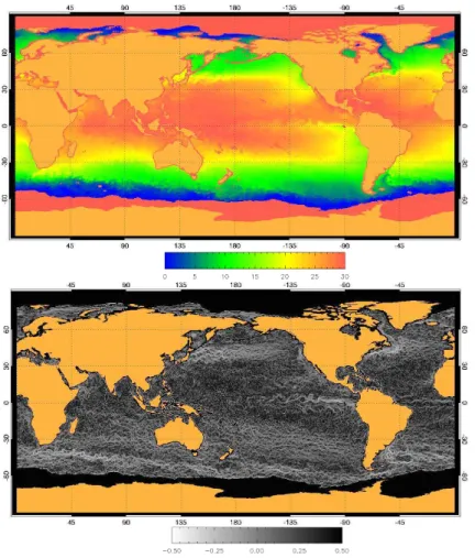
In Fig. 1 we show an example of singularity analysis on a global map of Microwave (MW) Sea Surface Temperature (SST); for details on the obtaining of singularity ex-ponents see Appendix A. Many hydrographic features of global and regional ocean circulation become evident in the singularity map. Main boundary currents, such as

15

the Gulf Stream, the Kuroshio, the Agulhas retroflection current or the Falkland cur-rent, as well as the diverse filaments of the Antartic Circumpolar Curcur-rent, which can be vaguely distinguished in SST maps, become clear and distinct in the singularity map, in addition with other emerging filaments, eddies and currents that were hidden in the SST maps. Notice that even accepting that singularity exponents serve to delineate

20

(8)

OSD

6, 129–151, 2009

A. Turiel et al.

Title Page

Tables Figures

◭ ◮

Back Close

Full Screen / Esc

Interactive Discussion 4 Comparison with altimetry

Although the singularity maps derived from MW SST that we have presented are ap-pealing and seem to be highly correlated with the geometrical arrangement of currents in oceans, we need to confirm their validity as current tracers. Hence, we need inde-pendent measurements to contrast the similitudes and to quantify the degree of

close-5

ness between ocean currents and the filaments shown in singularity maps. However, this is precisely the question: we have no synoptic maps of ocean currents. Never-theless, for a more than a year between 2002 and 2003 high-quality daily maps of geostrophic currents derived from the combination of four satellite altimeters are avail-able (Pascual et al., 2006). Hence, we have used these data, produced by CLS, as a

10

reference in the present study.

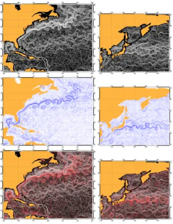
In Fig. 2 we show a couple of examples of the comparison of singularity maps derived from MW SST and high-quality altimeter maps, for two different regions. The visual as-sessment indicates that singularities align quite well with altimeter-derived geostrophic currents.

15

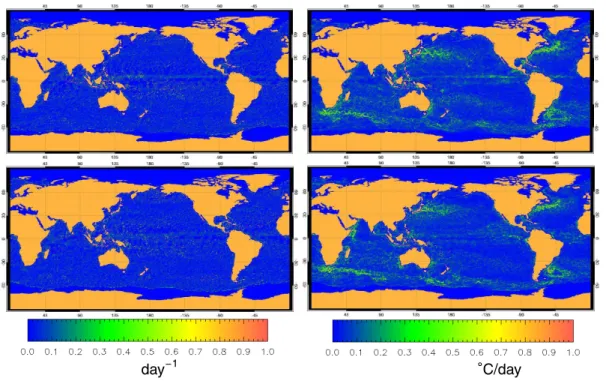
However, a simple visual comparison does not allow to quantify the degree of close-ness between altimeter-derived currents and singularity lines. Hence, we have esti-mated the advective and the material derivatives of the singularity exponentsh(x, t) us-ing the geostrophic velocity fieldv(x, t), that we denote byAh=v· ∇handDh=∂_th+Ah, respectively; processing details can be found in Appendix B. If the singularity

expo-20

nents delineate streamlines, then the advective derivative should be zero, Ah=0. If the singularity exponents are passive tracers, then the material derivative equals zero, Dh=0. In Figs. 3 and 4, we show examples of the computation of both types of deriva-tive in two different months of the year 2003; notice that in the figures we show the time average for the considered period of the absolute values of the time derivative.

25

For comparison purposes, we present the derivatives of both SST and singularity ex-ponents.

(9)

singu-OSD

6, 129–151, 2009

A. Turiel et al.

Title Page

Tables Figures

◭ ◮

Back Close

Full Screen / Esc

Interactive Discussion larity exponents, although advective derivatives are significantly smaller. This means

that the hypothesis that singularity exponents delineate streamlines is more consistent than the hypothesis of passive advection of singularity exponents. However, the partial time derivative of the singularity exponents, i.e. the term∂_th, is relatively small and so both types of derivative are not so different; hence, the hypothesis of passive

advec-5

tion of singularity exponents can be appropriate for short time periods. Comparing the results of the time derivatives of singularity exponents and those of SST is not straight-forward, as they do not have the same units. Time derivatives of SST seem to be much less uniform than those of singularity exponents and significantly greater in value, but lacking of an appropriate conversion unit the used colorbars are conventional and so

10

this conclusion is rather arbitrary. In fact, average advective derivatives of SST are of about 0.5◦C/day, which do not seem very large. To help comparison, we have de-fined new quantities with the same dimensions for both variables and informative about the quality as fluid tracers of each variable. We thus define the advective divergence speed,V_A, and the material divergence speed,V_M, of a scalarθas follows:

15

VA(x, t)≡

|Aθ(x, t)|

|∇θ(x, t)| , VM

(x, t)≡|Dθ(x, t)|

|∇θ(x, t)|

(3)

These quantities have units of speed, and we interpret them as the speeds at which the isolines ofθseparate from the actual streamlines. This interpretation is supported by the implicit function identity∂_tθ/∂_xθ=−∂_tx. A more precise argument in support of this interpretation is the following: the advective (vs. material) time derivative informs

20

us about the rate of variation of the variableθas we move along the streamline (vs. tra-jectory), but gives no idea about the distance that the water parcel has run to observe such an increment of the variable. On the other hand, the gradient ofθgives informa-tion about the spatial variability ofθgoing along the direction of fastest variation, which is always perpendicular to the isolines ofθ. Hence, the ratio of the time derivative by

25

(10)

OSD

6, 129–151, 2009

A. Turiel et al.

Title Page

Tables Figures

◭ ◮

Back Close

Full Screen / Esc

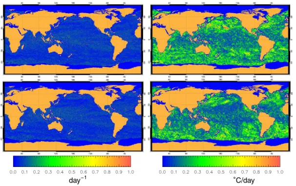
Interactive Discussion We show examples of divergence speeds in Figs. 5 and 6. Figures show that both

advective and material divergence speeds of singularity exponents have small values, which are of the order 1–2 km/day on average. In addition, divergence speeds are very uniformly distributed on the Globe, with more significant deviations on areas of larger mesoscale activity around the great boundary currents.

5

The situation is quite different for SST-derived divergence speeds. Advective diver-gence speeds are relative small on average (around 8 km/day) but less uniformly dis-tributed that their singularity counterparts. Material divergence speeds, on the other hand, have rather large values, of order 30 km/day on average, with peaks up to 50 km/day, and are more associated to some frontal areas and possibly to the

pres-10

ence of active upwelling/downwelling, which indeed changes the thermal signature on the affected areas.

5 Conclusions

We have shown that singularity analysis of MW SST images can be used to uncover the circulation patterns in global oceans. Singularity exponents are dimensionless

quanti-15

ties, and they are less affected by large-area effects like sun heating cycles, sunglint, etc. In addition, they have much richer spatial structure, with strong variations, what aids to give a precise location to mesoscale features like eddies and filaments. Results indicate that singularity exponents are appropriate to delineate instantaneous stream-lines with an average uncertainty of about 1 km/day, that is, around 1 cm/s. This value

20

of the divergence speed is the smallest possible one, as it is of the order of altimeter accuracy. This result means a significant improvement with respect to other techniques employed to extract dynamic information on SST such as MCC (Bowen et al., 2002) or Surface Quasi Geostrophy (Isern-Fontanet et al., 2006). However, singularity analysis does not provide access to the full velocity vector, just to its direction. The modulus

25

(11)

OSD

6, 129–151, 2009

A. Turiel et al.

Title Page

Tables Figures

◭ ◮

Back Close

Full Screen / Esc

Interactive Discussion the combination with the information of the forthcoming generation of wide-swath

al-timeters (Chelton, 2001) will mitigate such a limitation providing an improvement of the results.

As MW SST images are now produced at a daily rate, the techniques described in this paper are relevant for many purposes. At a operational level it can eventually

pro-5

duce high resolution operational instantaneous velocity fields. At a more fundamental level it enables a better use of the satellite information to study many oceanographic processes. We can easily determine the position of different fronts associated to the Antarctic Circumpolar Current, to quantify the extent and propagation speed of Tropi-cal Instability Waves or to study the filamentation of the great boundary currents and

10

how they close the great subtropical gyres at the eastern boundary. All those struc-tures are strongly linked to large-extent phenomena which condition the climate; the re-analysis of existing databases and the on-going produced maps will be useful to un-derstand the short-term variability of oceanic part of the climate engine and to improve our knowledge in future years.

15

Appendix A

Application of singularity analysis

For the determination of the singularity exponents we have employed as waveletΨan optimized numerical implementation of the Lagrangian wavelet,

20

ΨL(x)=

1 1+|x|2

(A1)

(12)

OSD

6, 129–151, 2009

A. Turiel et al.

Title Page

Tables Figures

◭ ◮

Back Close

Full Screen / Esc

Interactive Discussion to this purpose. In fact, it has been shown to have a good performance on real

situ-ations, although it truncates the singularities beyondh=0. To avoid this effect, which is connected with the behavior of the tail of the wavelet (Turiel et al., 2008b), we have constructed a numerical implementation,ΨLn, which is defined by a matrix of

numeri-cal weights which is close toΨLfor small values of|x|but has a faster decay for larger 5

values of|x|.

The exponentsh(x, t) are obtained by the application of Eq. (2) at different resolution scalesr. For a set of scalesr1,r2,. . .,rma linear regression of logTΨ[∇θ](x, r) vs. logr is performed at each pointxin the image; the slope of such a regression is the singular-ity exponenth(x). For the experiences shown in this paper we have usedm=7 different

10

scales which are uniformly sampled in a logarithmic axis, logri+1−logri=constant. We

fix the constant so thatr1=1 pixel andrm=0.1×image size.

Appendix B

Evaluation of time derivatives

15

For the determination of the advective and material derivatives of the different scalars we need to compute the Lagrangian trajectories, for which we have used a simple in-tegration scheme. Let us first introduce some notation. We will denote the longitude coordinate byφand the latitude coordinate byλ. For two points on the spherep=(φ, λ), p′=(φ′, λ′) we define the distance between them by the length of arc of geodesic

cir-20

cle which joints both points. For two points of close coordinates we approximate this distanced(p,p′) by the following expression:

d(p,p′) = R_e

s

(λ−λ′₎2₊_(φ₋_φ′₎2_cos2

λ+λ′ 2

(B1)

(13)

OSD

6, 129–151, 2009

A. Turiel et al.

Title Page

Tables Figures

◭ ◮

Back Close

Full Screen / Esc

Interactive Discussion Given a pointpin the sphere, we evaluate the velocity at that point by interpolating

the velocities of the four closest points. If the four first neighbors ofp on the velocity grid are the pointsq₁,q₂,q₃andq₄, we evaluate the velocity atpas follows:

v(p, t)= X

ivalid

Z

d(p,q_i) v(qi, t) (B2)

where the sum in the expression above is restricted to valid points (i.e. points on the

5

ocean with measured velocity) and the normalization constantZ is such that all the weights sum up to 1,

Z−1= X

ivalid

1

d(p,q_i) (B3)

When none of the four first neighbor points has a valid velocity we consider the pointp cannot be assigned a valid velocity.

10

A trajectory p(t) is constructed by integrating velocity maps, interpolated in both space and time, with one-hour time increments, that is:

p(t+ ∆t)=p(t)+v(p(t), t)∆t (B4)

where here∆t=1 h.

To compute the advective and material derivatives of a scalar θ(x, t) we need to

15

compute its increments along a trajectory for constant and time-varying maps, respec-tively. We evaluate the value of the scalarθ at a non-grid point p in a similar way to what is done with the velocity, namely:

θ(p, t)= X

ivalid

Z

(14)

OSD

6, 129–151, 2009

A. Turiel et al.

Title Page

Tables Figures

◭ ◮

Back Close

Full Screen / Esc

Interactive Discussion The interpolation on singularity exponents should be treated in a slightly different way,

however. When considering singularity exponentsh(x, t) it should be taken into ac-count that variablesh(x, t) are not additive and hence they cannot be linearly interpo-lated. According to Eq. (2), what is additive isrh(x,t), so we should hence interpolate h(p, t) according to the following expression:

5

rh(p,t)

= X

ivalid

Z d(p,q_i) r

h(qi,t) _(B6)

wherer is the resolution scale at which singularity exponents are calculated. The value ofr can be difficult to obtain in real situations, but we can take advantage of the fact it is very small in our case, so we can simplify the expression above by considering the dominant term,

10

h(p, t)=min_i_valid{h(q_i, t)} (B7)

that is, the exponent at the pointpis the minimum of the exponents of the valid neigh-boring points.

The advective derivative ofθat the pointp(t) and timet is given by the variation of θalong the trajectory for a constant map and time increment∆t=1 day, according the

15

equation:

Aθ(p(t), t)= θ(p(t+ ∆t), t)−θ(p(t), t)

∆t (B8)

while the material derivative is evaluated taking into account that the map θ itself evolves,

Dθ(p(t), t)= θ(p(t+ ∆t), t+ ∆t)−θ(p(t), t)

∆t (B9)

20

(15)

OSD

6, 129–151, 2009

A. Turiel et al.

Title Page

Tables Figures

◭ ◮

Back Close

Full Screen / Esc

Interactive Discussion at each timet we take each point in the ocean as the origin and we integrate for a

single time step∆t; the advective derivatives at the same point and different times are averaged together. In the case of the time-averaged material derivative, we take each point on the ocean grid as starting point of the respective trajectory, that we follow for all the days in the time period used to average, then the material derivatives starting

5

from the same point at the initial day are averaged together.

To avoid divergences due to cancellations in the gradient in Eq. (3), both the time derivative and the gradient are weighted with a fast-decreasing kernel, namely (1+|r|2)−1.

Acknowledgements. This is a contribution to the EU MERSEA project (AIP3-CT-2003-502885)

10

and to the Spanish projects OCEANTECH (PIF 2006 project) and MIDAS-4 (ESP2005-06823-C05-1).

References

Arneodo, A., Argoul, F., Bacry, E., Elezgaray, J., and Muzy, J. F.: Ondelettes, multifractales et turbulence, Diderot Editeur, Paris, France, 169 pp., 1995. 134

15

Bowen, M., Emery, W., Wilkin, J., Tildesley, P., Barton, I., and Knewtson, R.: Extracting multi-year surface currents from sequential thermal imagery using the Maximum Cross-correlation Technique, J. Atmos. Oceanic Technol., 19, 1665–1676, 2002. 131, 138

Chapron, B., Collard, F., and Ardhuin, F.: Direct measurement of ocean surface ve-locity from space: Interpretation and validation, J. Geophys. Res., 110, C0022,

20

doi:10.1029/2004JC0022, 2005. 130

Chelton, D. B.: Report of the High-Resolution Ocean Topography, Tech. rep., Science Work-ing Group MeetWork-ing Report, http://www.coas.oregonstate.edu/research/po/research/hotswg/, 2001. 139

Crocker, R., Emery, W., Matthews, D., and Baldwin, D.: Computing Ocean Surface Currents

25

from Infrared and Ocean Color Imagery, IEEE Trans. Geosci. Rem. Sens., 45, 435–447, 2007. 131

(16)

OSD

6, 129–151, 2009

A. Turiel et al.

Title Page

Tables Figures

◭ ◮

Back Close

Full Screen / Esc

Interactive Discussion

Frisch, U.: Turbulence, Cambridge Univ. Press, Cambridge MA, 312 pp., 1995. 135

Isern-Fontanet, J., Chapron, B., Lapeyre, G., and Klein, P.: Potential use of microwave sea surface temperatures for the estimation of ocean currents, Geophys. Res. Lett., 22, L24608, doi:10.1029/2006GL027801, 2006. 138

Isern-Fontanet, J., Turiel, A., Garcia-Ladona, E., and Font, J.: Microcanonical Multifractal

For-5

malism: application to the estimation of ocean surface velocities, J. Geophys. Res., 112, C05024, doi:10.1029/2006JC003878, 2007. 132, 134, 138

Johannessen, J., Kudryavtsev, V., Akimov, D., Eldevik, T., Winther, N., Johannessen, O., and Chapron, B.: On Radar Imaging of Current Features; Part 2: Mesoscale Eddy and Current Front detection, J. Geophys. Res., 110, C07017, doi:10.1029/2004JC002802, 2005. 130

10

Kraichnan, R.: Small-scale structure of a scalar field convected by turbulence, Phys. Fluids, 11, 945–963, 1968. 131

Lagerloef, G., Mitchum, G. T., Lukas, R. B., and Niiler, P. P.: Tropical pacific near surface currents estimated from altimeter, winds and drifter data, J. Geophys. Res., 104, 23313– 23326, 1999. 134

15

Lapeyre, G., Hua, B., and Klein, P.: Dynamics of the orientation of active and passive scalars in two dimensional turbulence, Phys. Fluids, 13, 251–264, 2001. 131

Larnicol, G., Guinehut, S., Rio, M.-H., Drevillon, M., Faugere, Y., and Nicolas, G.: The global observed ocean products of the French Mercator project, in: Proceedings of the “15 years of progress in Radar altimetry” ESA Symposium, ESA, Venice, 2006. 133

20

Mallat, S.: A Wavelet Tour of Signal Processing, Academic Press, 2nd Edition, 577 pp., 1999. 134

Nieves, V., Llebot, C., Turiel, A., Sol ´e, J., Garc´ıa-Ladona, E., Estrada, M., and Blasco, D.: Common turbulent signature in sea surface temperature and chlorophyll maps, Geophys. Res. Lett., 34, L23602, doi:10.1029/2007GL030823, 2007. 132, 134

25

Pascual, A., Faugere, Y., Larnicol, G., and Traon, P. L.: Improved description of the ocean mesoscale variability by combining four satellite altimeters, Geophys. Res. Lett, 33, 611, doi:10.1029/2005GL024633, 2006. 131, 133, 136

Reynolds, R. and Smith, T.: Improved global sea surface temperature analyses using optimal interpolation, J. Climate, 7, 929–948, 1994. 133

30

(17)

OSD

6, 129–151, 2009

A. Turiel et al.

Title Page

Tables Figures

◭ ◮

Back Close

Full Screen / Esc

2005. 133

Traon, P. L. and Dibarboure, G.: An illustration of the unique contribution of the TOPEX/Poseidon – Jason-1 tandem mission to mesoscale variability studies, Marine Geodesy, 27, 3–13, 2004. 133

Traon, P. L., Nadal, F., and Ducet, N.: An improved mapping method of multisatellite altimeter

5

data, J. Atmos. Oceanic Technol., 15, 522–534, 1998. 131

Traon, P. L., Faug `ere, Y., Hernandez, F., Dorandeuand, J., Mertz, F., and Ablain, M.: Can we merge GEOSAT Follow-On with TOPEX/POSEIDON and ERS-2 for an improved description of the ocean circulation?, J. Atmos. Oceanic Technol., 20, 889–895, 2003. 133

Turiel, A. and Parga, N.: The multi-fractal structure of contrast changes in natural images: from

10

sharp edges to textures, Neural Computation, 12, 763–793, 2000. 131, 134

Turiel, A., Grazzini, J., and Yahia, H.: Multiscale techniques for the detection of precipi-tation using thermal IR satellite images, IEEE Geosci. Remote Sens. Lett., 2, 447–450, doi:10.1109/LGRS.2005.852712, 2005a. 134

Turiel, A., Isern-Fontanet, J., Garc´ıa-Ladona, E., and Font, J.: Multifractal method for the

instan-15

taneous evaluation of the stream function in geophysical flows, Phys. Rev. Lett., 95, 104502, doi:10.1103/PhysRevLett.95.104502, 2005b. 132, 134, 138

Turiel, A., P ´erez-Vicente, C., and Grazzini, J.: Numerical methods for the estimation of multi-fractal singularity spectra on sampled data: a comparative study, J. Computat. Phys., 216, 362–390, 2006. 139

20

Turiel, A., Sol ´e, J., Nieves, V., Ballabrera-Poy, J., and Garc´ıa-Ladona, E.: Tracking oceanic currents by singularity analysis of Micro-Wave Sea Surface Temperature images, Rem. Sens. Environ., 112, 2246–2260, 2008a. 132, 134

Turiel, A., Yahia, H., and P ´erez-Vicente, C.: Microcanonical Multifractal Formalism: a geomet-rical approach to multifractal systems. Part I: Singularity analysis, J. Phys. A, 41, 015 501,

25

doi:10.1088/1751-8113/41/1/015501, 2008b. 135, 140

(18)

OSD

6, 129–151, 2009

A. Turiel et al.

Title Page

Tables Figures

◭ ◮

Back Close

Full Screen / Esc

(19)

OSD

6, 129–151, 2009

A. Turiel et al.

Title Page

Tables Figures

◭ ◮

Back Close

Full Screen / Esc

(20)

OSD

6, 129–151, 2009

A. Turiel et al.

Title Page

Tables Figures

◭ ◮

Back Close

Full Screen / Esc

day−1 ◦C/day

(21)

OSD

6, 129–151, 2009

A. Turiel et al.

Title Page

Tables Figures

◭ ◮

Back Close

Full Screen / Esc

day−1 ◦C/day

(22)

OSD

6, 129–151, 2009

A. Turiel et al.

Title Page

Tables Figures

◭ ◮

Back Close

Full Screen / Esc

km/day

(23)

OSD

6, 129–151, 2009

A. Turiel et al.

Title Page

Tables Figures

◭ ◮

Back Close

Full Screen / Esc

km/day