CPD
10, 1527–1565, 2014Paleoenvironmental reconstruction of the
last 15 000 cal yr BP
A. O. Badejo et al.
Title Page
Abstract Introduction
Conclusions References
Tables Figures
◭ ◮
◭ ◮
Back Close
Full Screen / Esc
Printer-friendly Version Interactive Discussion
Discussion
P
a
per
|
D
iscussion
P
a
per
|
Discussion
P
a
per
|
Discuss
ion
P
a
per
|
Clim. Past Discuss., 10, 1527–1565, 2014 www.clim-past-discuss.net/10/1527/2014/ doi:10.5194/cpd-10-1527-2014
© Author(s) 2014. CC Attribution 3.0 License.
Open Access
Climate of the Past
Discussions
This discussion paper is/has been under review for the journal Climate of the Past (CP). Please refer to the corresponding final paper in CP if available.
A paleoenvironmental reconstruction of
the last 15 000 cal yr BP via Yellow Sea
sediments using biomarkers and isotopic
composition of organic matter
A. O. Badejo1, B.-H. Choi1, H.-G. Cho2, H.-I. Yi3, and K.-H. Shin1
1
Department of Environmental Marine Sciences, Hanyang University, Ansan, 426-791, Korea
2
Department of Earth and Environmental Sciences and Research Institute of Natural Science, Gyeongsang National University, Jinju, 660-701, Korea
3
Marine Geoenvironmental Research Divisions, Korea Institute of Ocean Science and Technology (KIOST), Ansan, 425-170, Korea
Received: 6 March 2014 – Accepted: 3 April 2014 – Published: 9 April 2014
Correspondence to: K.-H. Shin (shinkh@hanyang.ac.kr)
CPD
10, 1527–1565, 2014Paleoenvironmental reconstruction of the
last 15 000 cal yr BP
A. O. Badejo et al.
Title Page
Abstract Introduction
Conclusions References
Tables Figures
◭ ◮
◭ ◮
Back Close
Full Screen / Esc
Printer-friendly Version Interactive Discussion
Discussion
P
a
per
|
D
iscussion
P
a
per
|
Discussion
P
a
per
|
Discuss
ion
P
a
per
|
Abstract
This study is the first reconstruction of the paleoenvironment and paleovegetation dur-ing the Holocene (interglacial) and glacial periods of the Yellow Sea. We report the carbon isotopic and biomarker (n-alkane and alkenone) compositions of organic matter from Yellow Sea sediments since the glacial period. Our findings show that the
variabil-5
ity of the East Asian Monsoon (EAM) affected the sedimentary profile of total organic carbon (TOC), the stable isotopes of bulk organic carbon (δ13Corg), the atomic ratio of carbon and nitrogen (C/N ratio), and biomarker content. The sedimentary δ13Corg profile along the core exhibited more negativeδ13Corg values under cold/dry climatic
conditions (Younger and Oldest Dryas). The carbon preference index (CPI), the
pris-10
tane to phytane ratio (Pr/Ph) and the pristane to n-C17 ratio (Pr/n-C17) were used to
determine the early stages of diagenesis along the sediment core. Two climatic condi-tions were distinguished (warm/humid and cold/dry) based on ann-alkane proxy, and the observed changes inδ13C of individualn-alkane (δ13CALK) between the Holocene
and glacial periods were attributed to changes in plant distribution/type. Clear diff
er-15
ences were not found in the calculated alkenone sea surface temperature (SST) be-tween those of the Holocene and glacial periods. This anomaly during the glacial period might be attributed to the seasonal water mass distribution in the Yellow Sea or a sea-sonal shift in the timing of maximum alkenone production as well as the Bølling/Allerød interstadial.
20
1 Introduction
The Yellow Sea, which is located in the northern portion of the East China Sea, is strongly influenced by the East Asian Monsoon (EAM) System. Important climate records for this region have been preserved. Monsoonal strength varied among the cir-culation pattern during the late Quaternary of the Yellow and East China Seas (YECS),
25
CPD
10, 1527–1565, 2014Paleoenvironmental reconstruction of the
last 15 000 cal yr BP
A. O. Badejo et al.
Title Page
Abstract Introduction
Conclusions References
Tables Figures
◭ ◮
◭ ◮
Back Close
Full Screen / Esc
Printer-friendly Version Interactive Discussion
Discussion
P
a
per
|
D
iscussion
P
a
per
|
Discussion
P
a
per
|
Discuss
ion
P
a
per
|
the interglacial period (An, 2000) as well as dry/wet oscillations during the glacial period (Xiao et al., 1998). Su (1998) described an apparent EAM climate controlled seasonal variation, whereas Li et al. (1997) and Jian et al. (2000) described an intensified EAM during the glacial period, which weakened the Kuroshio Current (KC) and strengthened the coastal currents. The EAM and the encroachment of the KC, (which is caused by
5
significant changes in seasonal variations of water mass circulation) primarily control the circulation pattern of the Yellow Sea (Fig. 1). The coastal current along the Chinese and Korean coasts flows southward during winter and northward during summer in re-sponse to the prevailing wind (Uehara and Saito, 2003). During winter, the shelf water column is nearly homogenous, whereas the density structure of water masses can be
10
modified during summer as a result of the freshwater discharge from the Changjiang (CDW), surface heating, and tidal mixing (Naimie et al., 2001).
When the sea level was lower than it is today during the glacial period, the winter monsoon winds controlled the EAM, whereas the summer monsoon winds controlled the EAM during the interglacial periods, creating cold/dry and warm/wet climatic
condi-15
tions during these periods, respectively. Based on these reports, we assumed that the seasonal variation of the circulation pattern of the YECS indirectly affects sedimenta-tion within the region.
Recent applications of paleoclimatology to reconstruct Asian paleomonsoon variabil-ity have been well documented elsewhere (Ishiwatari et al., 2001; Ijiri et al., 2005; Zhao
20
et al., 2006; Fujine et al., 2006; Yu et al., 2011; Khim et al., 2012). Oscillations in grain size and magnetic susceptibility between the late glacial and interglacial periods on the Chinese Loess Plateau over the last 179 kyr might have been caused by variability in the Asian paleomonsoon (Zhang et al., 2003). Others have indicated that the advance and retreat of the KC, which transports heat to the North Pacific, was associated with
25
the last glacial/interglacial cycle, which affected the climate and sea surface tempera-ture (SST) of the North Pacific (Sawada and Handa, 1998; Ternois et al., 2000).
CPD
10, 1527–1565, 2014Paleoenvironmental reconstruction of the
last 15 000 cal yr BP
A. O. Badejo et al.
Title Page
Abstract Introduction
Conclusions References
Tables Figures
◭ ◮
◭ ◮
Back Close
Full Screen / Esc
Printer-friendly Version Interactive Discussion
Discussion
P
a
per
|
D
iscussion
P
a
per
|
Discussion
P
a
per
|
Discuss
ion
P
a
per
|
reconstruction of the paleoenvironment and paleovegetation during the Holocene and glacial periods based on sedimentary biomarker content and stable isotope indicators from the Yellow Sea. This study used lipid biomarkers and the isotopic composition of OM from a sediment core dating to approximately 15 000 cal yr BP to understand the environmental changes in the Yellow Sea over the last 15 000 yr. We compared
5
our results with reported monsoon activity from this marginal sea in the Pacific Ocean to examine whether these environmental changes were related to regional climatic oscillations.
2 Geographical and geological settings
The Yellow Sea is a marginal sea in the northwest Pacific Ocean enclosed by the
10
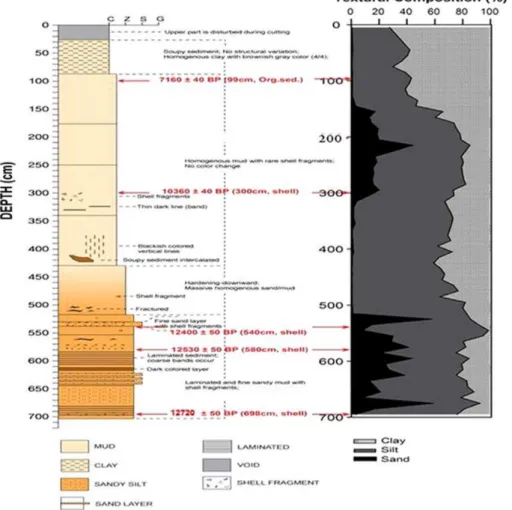
Chinese and Korean coasts and divided into the North and South Yellow seas by the Shandong Peninsula (Fig. 1). Muddy and sandy sediments predominate the Yellow Sea. Muddy sediment is primarily composed of silt and clay,whereas sandy sediment is composed of fine sand, silty sand and clayey sand (Fig. 2). The adjacent Yellow and Chagjiang rivers discharge sediments into the Yellow Sea (Uehara and Saito, 2003).
15
The Yellow Sea was subaerially exposed as a result of the reduction in sea level to approximately 120 m below its present level during the late glacial period. The sea-sonal variation of the different water masses controlled by the EAM climate and the encroachments of the KC sensitize the Yellow Sea to climatic change. The coastal cur-rent of the Yellow Sea flows southward in winter and northward in summer as a result
20
of the prevailing winds (Uehara and Saito, 2003). Along the shelf, the water column is approximately homogenous during winter, whereas the Changjiang River modifies the density structure and flow pattern in summer (Naimie et al., 2001). The Yellow Sea Warm Current (YSWC), an offshoot of the KC, is the only major water flow that trans-ports warm saline water from the open sea to the Yellow Sea and affects the water
25
CPD
10, 1527–1565, 2014Paleoenvironmental reconstruction of the
last 15 000 cal yr BP
A. O. Badejo et al.
Title Page
Abstract Introduction
Conclusions References
Tables Figures
◭ ◮
◭ ◮
Back Close
Full Screen / Esc
Printer-friendly Version Interactive Discussion
Discussion
P
a
per
|
D
iscussion
P
a
per
|
Discussion
P
a
per
|
Discuss
ion
P
a
per
|
3 Materials and methods
Sediment core 11 YS PCL 14, which was 702 cm long, was retrieved from the cen-tral Yellow Sea (latitude: 35◦785′N, longitude: 124◦115′E) for multi-proxy paleoenvi-ronmental reconstruction. This sediment core was sub-sampled at 10 cm intervals for carbon and nitrogen isotopic analysis and lipid biomarker analysis.
5
3.1 Experimental procedure
3.1.1 Age control
The age model for five selected depths (99, 300, 540, 580 and 698 cm) was deter-mined using accelerator mass spectrometer radiocarbon (AMS14C) data produced by the Beta Analytic Dating Laboratory, Miami, Florida. Details of the sample types are
10
shown in Table 1. The sediment samples were pre-treated with an acid wash (HCl) to remove carbonate and the shell fragment samples were pre-treated with an acid etch (deionized water and HCl). Conventional radiocarbon and calibrated ages are given in Table 1. Calibration were carried out using CALIB 7.0 program with the Marine04 cal-ibration curve database. All ages provided in the text refer to calibrated and calendar
15
ages. In order to obtain age-depth models the software Bacon version 2.2 (Blaauw and Cristen, 2011) was used (Fig. 3).
3.1.2 Bulk organic carbon analysis
Sixty-eight freeze dried and homogenized samples were submitted to Iso Analytical Ltd., UK, to analyze their carbon and nitrogen concentrations as well as stable isotope
20
compositions. Prior to these analyses, each 0.1 g sample was treated via acidification in 2 mL 10 % HCl for>12 h to allow for the liberation of CO2to remove carbonate carbon.
After the treatment, the sample was rinsed in deionized water, dried and transferred into tin capsules. To ensure quality control, each analysis included international standards 1A-R001 (wheat flour), 1A-R005 (beet sugar) and 1A-R006 (cane sugar) for carbon as
CPD
10, 1527–1565, 2014Paleoenvironmental reconstruction of the
last 15 000 cal yr BP
A. O. Badejo et al.
Title Page
Abstract Introduction
Conclusions References
Tables Figures
◭ ◮
◭ ◮
Back Close
Full Screen / Esc
Printer-friendly Version Interactive Discussion
Discussion
P
a
per
|
D
iscussion
P
a
per
|
Discussion
P
a
per
|
Discuss
ion
P
a
per
|
well as international standards 1A-R001, 1A-R045 (ammonium sulfate) and 1A-R046 (ammonium sulfate) for nitrogen. Isotope ratios were measured five times on three separate occasions with an instrumental measurement precision of±0.01 ‰ for carbon
and±0.03 ‰ for nitrogen. The reference standards were VPDB and air for carbon and
nitrogen, respectively.
5
3.1.3 Lipid extraction (biomarker analysis)
Sixty-eight dried and powdered samples were extracted using an Accelerated Solvent Extractor (ASE 200, Dionex Corp). The lipid extraction method was employed based on a previous study (Schwab and Sachs, 2009). Briefly, homogenized 10 g samples were extracted three times for 5 min with a mixture of dichloromethane and methanol
10
(DCM : MeOH, 9 : 1 v : v) under N2at 1500 psi and 150◦C. The solvents were removed under a stream of N2. The extracts were split into three different fractions using a
pre-combusted Al2O3 (6 h at 450◦C), deactivated with 5% H2O glass column
chromatog-raphy. The first fraction (F1) was eluted with hexane : DCM (9 : 1, v : v) and it contained hydrocarbons; F2 was eluted with hexane : DCM (1 : 1, v : v) and it contained alkenone;
15
polar fraction was eluted with DCM : MeOH (1 : 1, v : v). F2 was dried under a stream of N2and then derivatized with bis(trimethylsilyl)trifluoroacetamide (BSTFA) prior to in-strumental analysis. The alkenone fraction was derivatized so that the location of the double bond positions in C37-C40 alkenones can be differentiated.
Individual aliphatic (n-alkane) compounds (Fig. 4a) were identified and quantified
20
based on the retention time of the n-alkanes and the mass spectrum of selected ions with calibration standards using a GC-MS/FID (Shimadzu; GCMS-QP2010). The alkenones in F2 (Fig. 4b) were identified using a GC-MS (Shimadzu; GCMS-QP2010) to confirm the identity using the known ion chromatograms and by comparison with the GC trace identities provided by Dr. Antoni Rosell-Melé (ICREA, Barcelona, Spain).
25
CPD
10, 1527–1565, 2014Paleoenvironmental reconstruction of the
last 15 000 cal yr BP
A. O. Badejo et al.
Title Page
Abstract Introduction
Conclusions References
Tables Figures
◭ ◮
◭ ◮
Back Close
Full Screen / Esc
Printer-friendly Version Interactive Discussion
Discussion
P
a
per
|
D
iscussion
P
a
per
|
Discussion
P
a
per
|
Discuss
ion
P
a
per
|
The alkenone unsaturation index (UK37′) and temperature was calculated using the following equation (Prahl and Wakeham, 1987):
UK37′ =C37:2MK/(C37:2MK+C37:3MK)
UK37′ =0.034T +0.039.
5
3.1.4 Compound specificδ13Cn-alkanes
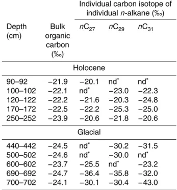
Based on the information obtained from the14C AMS dating and theδ13Corg analysis, five samples were selected from the climatic Holocene and glacial periods to study the changes in vegetation. Compound specificδ13C ofn-C27,n-C29, andn-C31were used
because these compounds were found in higher abundances than those of other long
10
chain alkanes.
Compound specific δ13C values of n-alkanes across 10 samples (Table 2) were determined using a coupled gas chromatograph-combustion-isotope ratio mass spec-trometer (GC-IRMS). A combustion interface with a copper oxide/platinum catalyst was connected to a Hewlett Packard 6890 N (Agilent Technology) gas chromatograph
15
equipped with a DB-5 fused capillary column (60 length, 0.032 mm i.d., and 0.25 µm film thickness; J & W Scientific). A hydrocarbon standard (C21) with a knownδ
13
C value was measured to assure the accuracy of the instrument. The standard deviation of the triplicate analyses of the standard was±0.3 ‰.
4 Results and discussion
20
4.1 Sediment lithology
CPD
10, 1527–1565, 2014Paleoenvironmental reconstruction of the
last 15 000 cal yr BP
A. O. Badejo et al.
Title Page
Abstract Introduction
Conclusions References
Tables Figures
◭ ◮
◭ ◮
Back Close
Full Screen / Esc
Printer-friendly Version Interactive Discussion
Discussion
P
a
per
|
D
iscussion
P
a
per
|
Discussion
P
a
per
|
Discuss
ion
P
a
per
|
of the sediment core (∼30–90 cm); a dark grayish mud with shell fragment remains
was found between approximately 90–430 cm deep; and homogenous sand/mud and some shell fragment remains predominated the lower part of the core (∼430–700 cm).
The textural composition of the sediments between approximately 150 and 300 cm consisted of sand/mud. The predominance of clay sediments in the upper portion of
5
the core indicated a low energy intertidal sedimentation regime. Grain size measure-ments, analyzed with regard to changes in EAM variability (Porter and An, 1995; Lu et al., 2000), indicated that a higher percentage of coarse grains were present dur-ing the glacial due to the strengthendur-ing of the winter monsoon, whereas finer particles predominated during the Holocene as a result of the strengthening of summer
mon-10
soon. Parallel laminated layers were observed between approximately 580 and 600 cm and 680 and 700 cm deep, which most likely reflect the deposition of OM under eux-inic/anoxic conditions caused by Yellow Sea exposure during the glacial period.
Calculated linear sedimentation rate by the age-depth model indicated that sedi-mentation rate was two times higher during the glacial (average 9.6 cm kyr−1) than the
15
Holocene (average 4.2 cm kyr−1). The large-scale changes in sea/land area and the rapid migration of the coastline in the glacial cycle must have had profound environ-mental significance (Wang, 1999). It is generally known that the rate of sedimentation is highest in basins where we have rivers. The Yellow Sea was exposed sub aerially and covered by a network of river channels during the glacial period
20
4.2 Sedimentary organic sources
Sedimentaryδ13Corgvaried from−25.84 to−21.61 ‰, with higher values found for the
Holocene and lower values discovered for the glacial. The C/N ratio varied from 6.15– 12.57. Low and high signatures of C/N values were recorded for the Holocene and glacial, respectively (Fig. 5). Higherδ13Corgvalues between−18 and−22 ‰ likely
orig-25
inate from marine OM (Middelburg and Nieuwenhuize, 1998), whereas lowerδ13Corg
CPD
10, 1527–1565, 2014Paleoenvironmental reconstruction of the
last 15 000 cal yr BP
A. O. Badejo et al.
Title Page
Abstract Introduction
Conclusions References
Tables Figures
◭ ◮
◭ ◮
Back Close
Full Screen / Esc
Printer-friendly Version Interactive Discussion
Discussion
P
a
per
|
D
iscussion
P
a
per
|
Discussion
P
a
per
|
Discuss
ion
P
a
per
|
Boot, 2004). Marine OM and terrigenous OM have C/N ratios of from approximately 5– 8 and >15, respectively (Meyers, 1997; Hu et al., 2009). The presence of inorganic nitrogen (IN), presumably in the form of adsorbed NH+4 on clay in surface deposits, can interfere with OM source identification when total nitrogen concentrations are low (Müller, 1977; Goñi et al., 1998; Datta et al., 1999; Kang et al., 2007; Hu et al., 2009).
5
Diagenetic processes most likely modify the original C/N ratios (Müller and Mathesius, 1999). However, based on the similar information provided by both proxies (δ13Corg and C/N) indicating a mixture of marine and terrigenous OM during the Holocene as well as terrigenous OM during the glacial the C/N ratio is a useful proxy to determine the source of OM in 11YS PCL14. Based on the EAM characteristics, a high influx of
10
terrestrial OM should have been delivered to the coastal and shelf sediments during the Holocene due to the large amounts of river discharge from the Yellow and Changjiang rivers caused by additional precipitation; however, the C/N ratio and δ13Corg indicate
otherwise. Specifically, these proxies indicate a mixture of terrigenous and marine or-ganic carbon during the Holocene as well as terrigenous oror-ganic carbon during the
15
glacial. Possible influences on the source of the organic carbon supply during these periods include the proportion of freshwater influx and sea level changes. The sed-imentation and burial of terrigenous OM is likely restricted to deltas and continental shelf areas; therefore, a minimal amount of terrigenous OM passed through the conti-nental slope to the deep sea (Hedges and Parker, 1976). Core 11YS PCL14 is located
20
in the central Yellow Sea (Fig. 1); therefore, it was not near the surrounding coastal environment. Thus, the core’s location greatly dilutes the terrigenous OM deposits via marine OM. The subaerial exposure of the Yellow Sea during the glacial period might have contributed to the formation of sand ridges, thereby explaining why bothδ13Corg and the C/N ratio indicated a terrigenous source of OM. Alin et al. (2008) found that
25
plant debris predominated sand from the continent.
CPD
10, 1527–1565, 2014Paleoenvironmental reconstruction of the
last 15 000 cal yr BP
A. O. Badejo et al.
Title Page
Abstract Introduction
Conclusions References
Tables Figures
◭ ◮
◭ ◮
Back Close
Full Screen / Esc
Printer-friendly Version Interactive Discussion
Discussion
P
a
per
|
D
iscussion
P
a
per
|
Discussion
P
a
per
|
Discuss
ion
P
a
per
|
during the early Holocene (∼11 000 to 10 000 cal yr BP) and then increases. The
oscil-lations of the TOC values along the sediment core might be due to changes in the sea level as well as related to the contribution of the autochthonous and allochthonous OM inputs that are also reflected in theδ13Corg and C/N signatures. These data indicate different types of OM during Holocene and glacial.
5
4.3 Depositional environment and OM preservation
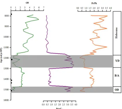
Pristane and phytane is derived from the geological alteration of the phytol side chain of chlorophyll-afrom algae, cyanobacteria and bacteria (Peters and Moldowan, 1993). The Pr/Ph ratio is typically used as a proxy for anoxic versus oxic bottom water con-ditions (i.e. redox changes) (Sawada, 2006). Pr/Ph ration values<1 indicate anoxic
10
environmental conditions for OM deposition, high values (>3) indicate oxic conditions of deposition (Didyk et al., 1978, Peters and Moldowan, 1993, Sawada, 2006), and val-ues of∼1 indicate alternating oxic and anoxic conditions of OM deposition (Didyk et
al., 1978; Hossain et al., 2009). In addition, the ratio of pristane to short chainn-alkane (Pr/n-C17) has been used to determine microbial activity, with values>1 indicating
15
strong microbial activity (González-Vila et al., 2003). Normal hydrocarbon (n-C17) is
easily degraded, and the resistant isoprenoids (pristane and phytane) are conserved, thereby resulting in a relative increase in the Pr/n-C17 ratio. The low Pr/Ph values and the high values of Pr/n-C17 values shown in Fig. 6 from the glacial period (Younger
and Oldest Dryas) likely indicates euxinic/anoxic sedimentary deposition conditions
20
with high bacterial activity, whereas high Pr/Ph values and low Pr/n-C17 values in-dicate oxic sedimentary deposition conditions and less bacterial activity. ten Haven et al. (1987) reported some limitations in the application of Pr/Ph ratio in oxicity of the en-vironmental of deposition. However the corroboration of parallel laminated layers with the Pr/Ph ratio at depths of 580 and 600 cm and 680 and 700 cm indicates a reducing
25
CPD
10, 1527–1565, 2014Paleoenvironmental reconstruction of the
last 15 000 cal yr BP
A. O. Badejo et al.
Title Page
Abstract Introduction
Conclusions References
Tables Figures
◭ ◮
◭ ◮
Back Close
Full Screen / Esc
Printer-friendly Version Interactive Discussion
Discussion
P
a
per
|
D
iscussion
P
a
per
|
Discussion
P
a
per
|
Discuss
ion
P
a
per
|
high bacterial activity was a result of nutrient supply, dissolved gases, and particulate organic and inorganic materials in surface melt water.
The CPI is a mathematical expression of the odd to even predominance between
n-C24 andn-C34. The CPI can be used as a proxy for the preservation potential of OM when a clear predominance of a superior plant wax exists (Ortiz et al., 2004).
How-5
ever, the CPI can also indicate the contribution of different OM sources (Pearson and Eglinton, 2000). CPI values of approximately 7 suggest the presence of young vascular plants, whereas values close to 1 are due to diagenetic processes (Hedges and Prahl, 1993). The CPI along the core (Fig. 6) showed two distinct OM states between the two climatic periods, with low values indicating high diagenetic processes of OM during the
10
Younger and Oldest Dryas and high values indicating less diagenetic processes dur-ing the Holocene. One explanation for the CPI distribution profile along the sediment core might be related to the differences in the nature of the OM (i.e. the composition of terrigenous OM), its molecular structure, and the environmental conditions to which fluvial OM was subjected between the climatic periods.
15
A comparison between the CPI andδ13Corg, revealed that the former indicated
ter-rigenously derived OM, which contradicted the implications of the δ13Corg data. One
explanation of the CPI distribution profile along the sediment core might simply be re-lated to the nature of the OM. The presence of nitrogen-poor cellulose in marine OM allows this type of OM to be easily degraded or altered compared with terrigenous OM,
20
which is composed of lignin, and thus has a higher resistance to degradation and alter-ation. This explanation is also supported by the Pr/Ph and Pr/n-C17ratios, which
indi-cates the low preservation of marine OM during oxic environmental conditions and low bacterial activity compared with that of terrigenous OM. Post-depositional diagenesis also affects carbon isotope ratios. However, a less than 2 ‰ isotopic shift is expected
25
CPD
10, 1527–1565, 2014Paleoenvironmental reconstruction of the
last 15 000 cal yr BP
A. O. Badejo et al.
Title Page
Abstract Introduction
Conclusions References
Tables Figures
◭ ◮
◭ ◮
Back Close
Full Screen / Esc
Printer-friendly Version Interactive Discussion
Discussion
P
a
per
|
D
iscussion
P
a
per
|
Discussion
P
a
per
|
Discuss
ion
P
a
per
|
4.4 Paleoenvironmental interpretation
4.4.1 Long chainn-alkanes as indicators of paleovegetation types
Among terrigenous biomarkers, long chain n-alkanes are examples of lipids derived from leaf waxes found in marine sediments. Long chainn-alkanes from higher plants are used as higher plant biomarkers because they are relatively resistant to
biochem-5
ical degradation and diagenesis in sedimentary records. The carbon number of the compound with the maximum concentration of long chainn-alkanes can indicate vege-tation type (Cranwell, 1973; Zhang et al., 2006; Rao et al., 2011). Woody plants display
n-alkane distributions dominated by C27 or C29, whereas grasses are dominated by C31. Several indices have been used to study shifts in vegetation over time.
Exam-10
ples of these indices include the following ratios: (C23+C25)/(C23+C25+C29+C31),
which indicates terrigenous/emergent and submerged/floating plants; C23/C29, which discriminates between sphagnum/non-sphagnum; and C27/C31, which indicates the
relative proportion of woody plant/grass vegetation (Ficken et al., 2000; Nichols et al., 2006; Wang et al., 2012).
15
Modern molecular organic geochemistry studies have demonstrated that the ratio of C27/C31 n-alkanes and the n-alkane average chain length (ACL) of higher plants
(i.e. the average number of carbon atoms based on the abundance of the odd car-bon numberedn-alkanes) can be used to indicate woody plants and grassy vegeta-tion because leaf lipids derived from grasslands differ from those from forest plants
20
(Cranwell, 1973). The ACL distribution is also generally related to latitude (Poynter and Eglinton, 1990). Herbaceous plants tend to be dominated byn-C31. Cranwell (1973)
and Cranwell et al. (1987) reported that C27 and C29 chain lengths predominate in
woody plants. The distribution of higher plants along core 11YS PCL14 displayed a pattern of n-alkane compounds that differed between the two climatic periods, with
25
n-C27 predominant during the Holocene and n-C31 more prevalent during the glacial
CPD
10, 1527–1565, 2014Paleoenvironmental reconstruction of the
last 15 000 cal yr BP
A. O. Badejo et al.
Title Page
Abstract Introduction
Conclusions References
Tables Figures
◭ ◮
◭ ◮
Back Close
Full Screen / Esc
Printer-friendly Version Interactive Discussion
Discussion
P
a
per
|
D
iscussion
P
a
per
|
Discussion
P
a
per
|
Discuss
ion
P
a
per
|
variation during the Holocene or glacial. This is because there could be the possibil-ity of n-C29 in woody plants and herbaceous plants (Rao et al., 2011), indicating a mixed source plant type. Based on Schwark et al. (2002) and Wang et al. (2012), a highn-C27/n-C31 value reflects a greater contribution of woody plants growing under
warm/humid conditions, whereas low n-C27/n-C31 values indicate grassy vegetation
5
growing under cold/dry environmental conditions. The ACL in woody plants decreases under humid conditions (Oros et al., 1999). Oscillation of ACL showed an inverse corre-spondence with then-C27/n-C31 (Fig. 8). A similar and accurate interpretation can be
made with regard to then-C27/n-C31ratio. Then-C27/n-C31ratio can be applied to de-termine the relative proportion of woody plant/grass vegetation because of the possible
10
variation in long chain n-alkanes within the same plant under different environmental conditions (temperature and moisture changes). This ratio can also be applied to de-termine the composition and types of vegetation sources. For example, submergent macrophytes usually maximize atn-C23 orn-C25 but not atn-C27, whereas emergent
macrophytes have n-alkane distributions similar to terrigenous plants, maximizing at
15
n-C27, n-C29, or n-C31 (Cranwell, 1984; Ficken et al., 2000). We also sought to
vali-date the application of then-C27/n-C31 ratios for paleovegetation studies in the Yellow
Sea by examining the relationship between the geochemical proxies and the pollen records from the Okinawa Trough because these records are not available for the Yel-low Sea. The Zheng et al. (2012) pollen record indicated that conifer saccate pollen,
20
principally Pinus and Tsuga, predominated in most portions of the core, particularly the interglacial, whereas the herb pollen Cyperaceae was highly prevalent during the late glacial period.n-C27/n-C31, and ACL, indicates that disparate vegetation covered
different climatic periods.
4.4.2 Compound specificδ13C compositions ofn-alkanes
25
The compound specific isotopic composition of individualn-alkanes has been used to provide additional information regarding the changes in C3 and C4 vegetation cover.
CPD
10, 1527–1565, 2014Paleoenvironmental reconstruction of the
last 15 000 cal yr BP
A. O. Badejo et al.
Title Page
Abstract Introduction
Conclusions References
Tables Figures
◭ ◮
◭ ◮
Back Close
Full Screen / Esc
Printer-friendly Version Interactive Discussion
Discussion
P
a
per
|
D
iscussion
P
a
per
|
Discussion
P
a
per
|
Discuss
ion
P
a
per
|
photosynthetic pathways were retained (Collister et al., 1994). Long chain n-alkanes produced by C3and C4plants showedδ
13
C values of−32 to−39 ‰ and−18 to−25 ‰,
respectively (Collister et al., 1994). The δ13CALK from core 11YS PCL14 (Table 2)
varied from−20 to−26 ‰ during the Holocene and from −30.1 to −43 ‰ during the
glacial. Theδ13Corgshowed higher values than theδ 13
CALK, particularly for the glacial
5
period (Table 2). The differences between δ13Corg and δ13CALK is as a result of lipid biosynthesis that leads to the additional isotopic fractionation against13C that occurs during the enzymatic decarboxylation of pyruvate to form acetate (DeNiro and Epstein, 1977). Large differences were observed in theδ13CALKvalues between the Holocene
and the glacial, althoughn-C27,n-C29, andn-C31 are apparently of terrigenous origin.
10
The shift in the13C of n-alkanes might be related to a change in floral assemblages from a C3 to a C4dominated assemblage. In sample 700–702 cm (Table 2), the δ
13
C values ofn-C31 are much more negative (−43 ‰) than those of n-C27 and n-C29. In
addition, in sample 690–692 cm, theδ13C values ofn-C31are less negative than those
ofn-C27 andn-C29. Smith et al. (2007) and Diefendorf et al. (2010) both reported that
15
gymnospermn-alkanes are more enriched in13C compared with then-alkanes of an-giosperms grown under the same climatic conditions.
However, most studies have attributed the highδ13Corgvalues of OM in African lake
sediments to the spread of C4 plants (savannah grasses and sedges) due to a drier climate, lowerpCO2, or both (Ficken et al., 1998; Huang et al., 1999). The results from
20
then-C27/n-C31, ACL,δ 13
Corg, andδ 13
CALKcontradicted this mechanism. A C4
path-way involves a CO2 concentrating mechanism through which CO2 initially combines with phosphoenol pyruvate to form a 4 carbon acid(oxaloacetate) (Collatz et al., 1998). This mechanism provides C4plants with a competitive advantage under lowpCO2
con-ditions. Several environmental conditions affecting the growth of C4 plants have been
25
proposed. C4 plants are more water efficient than C3plants (Ehleringer et al., 1991).
Teeri and Stowe (1976) suggested that C4 plants are more tolerant to aridity than C3
CPD
10, 1527–1565, 2014Paleoenvironmental reconstruction of the
last 15 000 cal yr BP
A. O. Badejo et al.
Title Page
Abstract Introduction
Conclusions References
Tables Figures
◭ ◮
◭ ◮
Back Close
Full Screen / Esc
Printer-friendly Version Interactive Discussion
Discussion
P
a
per
|
D
iscussion
P
a
per
|
Discussion
P
a
per
|
Discuss
ion
P
a
per
|
in low-latitude Africa and Mesoamerica, attributing this expansion to lowerpCO2levels, aridity, or both (Boom et al., 2002; Huang et al., 2001; Mora et al., 2002). Therefore, our results suggest that C4 plants were dominant during the Holocene, that C3 plants
predominated during the Younger and Oldest Drays, and that an expansion of C4plants occurred during the glacial interstadial (Bølling/Allerød). Similar vegetation distributions
5
andδ13CALKduring the interglacial and glacial periods were reported with regard to the
Chinese Loess Plateau (Zhang et al.,2003). The ACL, then-C27/n-C31 ratio and theδ
13
CALK displayed different profiles during
the Bølling/Allerød period compared with those from the Younger and Oldest Dryas. The Bølling/Allerød interstadial was a warm and humid climatic period that occurred
10
at the end of the late glacial period, beginning with the termination of a cold period (Oldest Dryas) and ending with the start of another cold period (Younger Dryas).
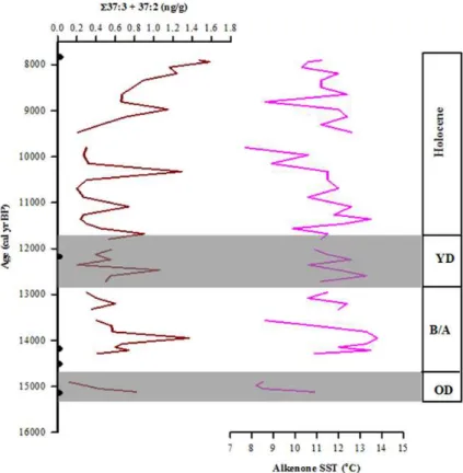
5 Alkenone abundance
As Fig. 8 illustrates, the concentration of C37:2+C37:3 ranged from 0.12–1.58 (ng g− 1
dry sediment). The C37:2+C37:3alkenone content (ng g− 1
dry sediment) was relatively
15
high during the Holocene compared with that of the glacial. The strong variation in alkenone concentrations was related to their production via haptophyte algae and the preservation or dilution of the molecules in the sedimentary matrix. The distribution of alkenones is likely a function of the physiological response of environmental alkenone producers such as temperature, salinity, and nutrient availability as well as the inputs
20
from different haptophyte populations with distinct biochemical signatures. As particu-late OM descends through the water column and is incorporated into the sediments, lipid biomarkers likely encounter different degradation conditions (Teece et al., 1998; Sinninghe Damsté et al., 2002).
Alkenones are more resistant to degradation than most other lipids of planktonic
ori-25
CPD
10, 1527–1565, 2014Paleoenvironmental reconstruction of the
last 15 000 cal yr BP
A. O. Badejo et al.
Title Page
Abstract Introduction
Conclusions References
Tables Figures
◭ ◮
◭ ◮
Back Close
Full Screen / Esc
Printer-friendly Version Interactive Discussion
Discussion
P
a
per
|
D
iscussion
P
a
per
|
Discussion
P
a
per
|
Discuss
ion
P
a
per
|
alkenone content between the Holocene and glacial. Rather, this phenomenon might be a result of differences in the dilution of the molecules in the sedimentary matrix and the alkenone production of haptophytes between the two climatic periods. Thunell et al. (1992) suggested that dilution with terrigenous sediment controlled the changes in the bulk carbonate content in South China Sea sediments during the glacial/interglacial
5
time period in response to sea level changes.
5.1 Alkenone based temperature (UK37′ SST)
Alkenone SST fluctuated from 7.7 to 14.1◦C in sediment core 11YS PCL14. The UK′
37
derived temperatures in the central Yellow Sea during the glacial/Holocene did not show clear variations (Fig. 8).
10
Two low UK37′SST values (160–162 and 220–222 cm) were recorded for the Holocene. These low values might be related to the cold events recorded in the North Atlantic deep-sea cores. Bond et al. (1997) reported a series of cold climate events during the middle and late Holocene and related these periods to ice rafted debris (IRD) events.
UK37′ derived temperatures during the Holocene and glacial periods displayed
fluc-15
tuations along the core. One simple explanation for these fluctuations might be the seasonal variation of water mass circulation. During winter, the YSWC flows at deep depths to the north of the Yellow Sea and becomes less intrusive during summer when the CDW intrudes into the Yellow Sea. The differences in the hydrological properties of the water masses of the Yellow Sea play a major role in the evolution of its marine
or-20
ganisms. This effect is reflected in the different alkenone temperatures at which these organisms grow during each season. Low alkenone derived SSTs were expected dur-ing the glacial period as a result of the regional cooldur-ing that was enhanced by the East Asian Winter Monsoon. However, high alkenone derived SSTs were observed for the glacial period. During the glacial period, the intrusion of the KC (which transports large
25
CPD
10, 1527–1565, 2014Paleoenvironmental reconstruction of the
last 15 000 cal yr BP
A. O. Badejo et al.
Title Page
Abstract Introduction
Conclusions References
Tables Figures
◭ ◮
◭ ◮
Back Close
Full Screen / Esc
Printer-friendly Version Interactive Discussion
Discussion
P
a
per
|
D
iscussion
P
a
per
|
Discussion
P
a
per
|
Discuss
ion
P
a
per
|
primary production and high UK37′derived temperatures. The unusually high UK37′derived temperatures during the glacial period were also reported for the Japan Sea (Ishiwatari et al., 2001; Fujine et al., 2006), the South China Sea (Zhao et al., 2006), and the Sea of Okhotsk (Seki et al., 2004). These studies reported various factors that affected or controlled the anomalously high UK37′ derived temperatures during the glacial period.
5
The unusually high UK37′ derived temperatures for the central region of the Yellow Sea during the glacial period are discussed below.
5.2 Ecological control regarding the estimation of UK37′ derived temperature
Ishiwatari et al. (2001) described four problems related to estimating alkenone based SSTs: (a) the effect of haptophyte species on alkenone SSTs; (b) the effects of post
10
deposition conditions on alkenone SSTs; (c) the salinity effects on alkenone SSTs; and (d) the shifts in haptophyte microalgae with climatic regime changes.
No microscopic observations of the haptophytes in our samples were made, so we cannot state conclusively that the usually high UK37′ derived temperatures during the glacial period were related to the effect of the haptophyte species on alkenone SST. The
15
highest relative C37:4% abundances from the total alkenone content were found in
re-gions with less salinity (Rosell-Melé, 1998; Sikes and Sicre, 2002). Rosell-Melé (1998) found a similar relationship between low salinities and usually high SSTs, with high C37:4% found in North Atlantic cores. In our study, the salinity effects on the alkenone
SSTs during the glacial period were also less likely because the C37:4 alkenone
abun-20
dance in core 11YS PCL14 was below the detection limit. This result suggests that salinity variations did not affect alkenone production in the central region of the Yellow Sea.
The presence of sea ice prevents haptophyte productivity by preventing light pen-etration into the surface water. Therefore, Seki et al. (2004) suggested that the high
25
CPD
10, 1527–1565, 2014Paleoenvironmental reconstruction of the
last 15 000 cal yr BP
A. O. Badejo et al.
Title Page
Abstract Introduction
Conclusions References
Tables Figures
◭ ◮
◭ ◮
Back Close
Full Screen / Esc
Printer-friendly Version Interactive Discussion
Discussion
P
a
per
|
D
iscussion
P
a
per
|
Discussion
P
a
per
|
Discuss
ion
P
a
per
|
period in autumn) and the equilibrium of thermal energy caused by the penetration of solar radiation into stratified surface seawaters during the LGM in the Japan Sea (Ishi-watari et al., 2001). Another factor that could have affected the recorded high alkenone SSTs during the glacial is the Bølling/Allerød a period of warm and humid climatic period that occurred at the end of the late glacial period.
5
6 Monsoon variability
The strength of the KC varied between the climatic periods. Due to the differences in the intensity of both the EAM and KC between the glacial and Holocene, the paleo-ceanographic conditions in the Yellow Sea should differ during the glacial period com-pared with those of today. The grain size, TOC,δ13Corg, C/N ratio, biomarker molecule
10
proxy and alkenone derived SST records from core 11YS PCL14 provide insight into the environmental changes that occurred in the Yellow Sea’s regional environmental dynamics from approximately 15 000 cal yr BP to the present, as inferred by EAM vari-ability.
The particle size distribution of the sediment lithology indicated different types of
15
EAM activity between the glacial and Holocene cycles. Finer particles suggest a wet/warm climate during the Holocene with strong summer monsoons, whereas coarse particles indicate a cold/dry climate during the glacial period predominated by strong winter monsoons. A study of the evolution of the tidal current field in the YECS with regard to sea level increases since the last glacial period (Uehara and Saito, 2003)
20
posited that sand ridges were formed as a result of extremely intense tidal bottom stress when the sea level was low. The formation of mud deposition was a result of the weak bottom stress as the sea level rose.
Increasing values of TOC,δ13Corg, and C37:2+C37:3 alkenones as well as
decreas-ing C/N ratios found in sediments during the Holocene indicated that a long term trend
25
CPD
10, 1527–1565, 2014Paleoenvironmental reconstruction of the
last 15 000 cal yr BP
A. O. Badejo et al.
Title Page
Abstract Introduction
Conclusions References
Tables Figures
◭ ◮
◭ ◮
Back Close
Full Screen / Esc
Printer-friendly Version Interactive Discussion
Discussion
P
a
per
|
D
iscussion
P
a
per
|
Discussion
P
a
per
|
Discuss
ion
P
a
per
|
during the glacial period (indicated by values of TOC and C37:2+C37:3 alkenones as well as decrease inδ13Corg and increased C/N ratios) might be linked to strong
win-ter monsoons. The low primary productivity of surface wawin-ter during the glacial period most likely occurred as a result of the weakened intrusion of the KC and the increasing dominance of the coastal waters (which is related to the intensified East Asian Winter
5
Monsoon). Water surface productivity over glacial/Holocene time scales was likely af-fected by dilution with terrigenous sediments during the glacial period in response to the sea level changes indicated by theδ13Corg values and C/N ratios. Zhao et al. (2006)
found less carbonate content for the glacial period and related it to the lower sea level that might have enhanced the transport of terrigenous sediments into the South China
10
Sea, thereby diluting the carbonate content. In contrast, high carbonate content should have been present during warm Holocene period with a higher sea level when most terrigenous sediments were trapped in estuaries or on the inner shelf.
The Pr/Ph ratios and the series of laminated thin, dark layers observed in the sedi-ment lithology corresponding to the glacial period indicated an anoxic environsedi-ment that
15
likely resulted from a lowered global sea level, which limited surface water exchange between the neighboring seas. Tada et al. (1995, 1999) stated that the formation of the dark layers during late Quaternary sequences in the Japan Sea was synchronized with Dansgaard–Oeschger (D–O) cycles, thereby attributing these layers to millennial-scale variations in the northern portion of the East China Sea during cold/dry climate periods.
20
Studying plant response to past global changes provides valuable insight to predict future responses to a rapidly changing environment (Ward et al., 2005; Jackson, 2007). Zhang et al. (2003) showed that lower temperatures were the primary cause of the C4 plant decline on the Chinese Loess Plateau during glacial period. Furthermore, the at-mospheric CO2concentration was low, and the climate was colder and drier, which led
25
to a shift to C3plants during these periods. This shift corroborates our reconstruction based on theδ13CALK. The shift in vegetation type at our study site was the result of the
CPD
10, 1527–1565, 2014Paleoenvironmental reconstruction of the
last 15 000 cal yr BP
A. O. Badejo et al.
Title Page
Abstract Introduction
Conclusions References
Tables Figures
◭ ◮
◭ ◮
Back Close
Full Screen / Esc
Printer-friendly Version Interactive Discussion
Discussion
P
a
per
|
D
iscussion
P
a
per
|
Discussion
P
a
per
|
Discuss
ion
P
a
per
|
and C4 plants. Therefore, we conclude that regional climatic variations controlled the vegetation changes during these climatic periods.
A study by Ijiri et al. (2005) indicated that the intensities of the KC and Asian Mon-soon varied between the glacial and interglacial periods, and these variations were the primary mechanisms responsible for the paleoceanographic variations in the East
5
China Sea. The weakening of the KC (which caused in an increasing dominance of coastal water) was attributed to the intensified East Asian Winter Monsoon during the glacial period. The change in the strength and path of the KC during the glacial pe-riod is a controversial topic (Sawada and Handa 1988; Kawahata and Ohshima, 2004); nevertheless, evidence from planktonic foraminifera and the pollen assemblages of
10
P. obliquiloculatata(Xu and Oda, 1999; Kawahata and Ohshima, 2004) suggest that
the KC entered the East China Sea during the glacial period. Based on our results, the unusually high UK37′ derived temperatures during the glacial period were most likely caused by an intrusion of the weakening KC as a result of weaker Summer Monsoon in the Yellow Sea and the warm period during the glacial (Bølling/Allerød).
15
7 Conclusions
The results from this study illustrated the variability of the EAM from approximately 15 000 cal yr BP to the present given the transition from the winter monsoon (cold/dry climate) to the summer monsoon (warm/wet climate) during the glacial and the Holocene. These notable findings were based on records of bulk geochemical
param-20
eters, terrigenous biomarkers and UK37′ derived SST from core 11YS PCL14 and are summarized below.
Distinct differences were observed in the TOC content within climatic periods. These differences were characterized by high values during the Holocene and lower values during the Oldest Dryas and Bølling/Allerød periods. The difference in the TOC
pat-25
CPD
10, 1527–1565, 2014Paleoenvironmental reconstruction of the
last 15 000 cal yr BP
A. O. Badejo et al.
Title Page
Abstract Introduction
Conclusions References
Tables Figures
◭ ◮
◭ ◮
Back Close
Full Screen / Esc
Printer-friendly Version Interactive Discussion
Discussion
P
a
per
|
D
iscussion
P
a
per
|
Discussion
P
a
per
|
Discuss
ion
P
a
per
|
terrigenous, glacial=terrigenous) as indicated by the δ13Corg values and the
down-core C/N ratios that were associated with the change in sea level.
δ13CALKwas used to reconstruct vegetation type, and atmospheric CO2was inferred
from this reconstruction. The results suggested that values ofδ13CALKwere attributed
to a different photosynthetic response to CO2and temperature among C3and C4plants
5
during the glacial period compared with the interglacial period. Then-C27/n-C31ratios
ofn-alkanes andδ13CALKindicated a change in vegetation from C4woody plants
dur-ing the Holocene to C3grassy plants during the glacial period and C4expansion in the glacial interstadial (Bølling/Allerød). Therefore, C4and C3plants were predominated in
warm/humid and cold/dry environmental conditions, respectively. Globally lowerpCO2
10
and regionally higher aridity likely favored the growth of C3 vegetation over C4 plants during the glacial period. We conclude that regional climate variables controlled the C3/C4 vegetation changes during the glacial/Holocene transition. Caution should be
taken when applying n-C27/n-C31 ratios due to the possibility of mixed effects from different sources ofn-C27 andn-C31.
15
Surface water productivity, represented by TOC,δ13Corg, and alkenone content,
in-creased during the Holocene and was influenced by the summer monsoon climate (warm/wet) due to its response to a relatively rapid rise in sea level. Surface water pro-ductivity was low during the glacial period during which a cold/dry climate influenced by the winter monsoon weakened the KC. The sedimentary dilution of terrigenous OM
20
also affected surface water productivity during the glacial period.
In accordance with other studies, grain size indicated a monsoonal variation, from coarse particles under the influence of the winter monsoon to fine particles during the summer monsoon. The presence of a laminated thin layer suggested an anoxic environment of sedimentary deposition as well as a correlation between the EAM and
25
D–O cycles during the glacial periods.
CPD
10, 1527–1565, 2014Paleoenvironmental reconstruction of the
last 15 000 cal yr BP
A. O. Badejo et al.
Title Page
Abstract Introduction
Conclusions References
Tables Figures
◭ ◮
◭ ◮
Back Close
Full Screen / Esc
Printer-friendly Version Interactive Discussion
Discussion
P
a
per
|
D
iscussion
P
a
per
|
Discussion
P
a
per
|
Discuss
ion
P
a
per
|
production during a shorter summer, the equilibrium of thermal energy caused by pen-etrations of solar radiation in stratified surface seawater and the Bølling/Allerød during the glacial period. Together with evidence concurrently indicating high SSTs during the glacial period, the unusually high UK37′ SSTs values during the glacial period are a signature of the marginal seas of the northwest Pacific Ocean.
5
Acknowledgements. The research project, “Geological Structure and Marine Geological Sur-vey in the Korean Jurisdictional Area” at the Korea Institute of Marine Science and Technology (KIMST) supported this study under the contract PJT200482.
References
Alin, S. R., Aalto, R., Goñi, M. A., Richey, J. E., and Dietrich, W. E.: Biogeochemical character-10
ization of carbon sources in the Strickland and Fly rivers, Papua New Guinea, J. Geophys. Res., 113, F01S05, doi:10.1029/2006JF000625, 2008.
An, Z.: The history and variability of the East Asian paleomonsoon climate, Quaternary Sci. Rev., 19, 171–187, 2000.
Blaauw, M. and Christen, J. A.: Flexible paleoclimate age-depth models using an autoregres-15
sive gamma process, Bayesian Anal., 6, 457–474, 2011.
Bond, G., Showers, W., Cheseby, M., Lotti, R., Almasi, P., deMenocal, P., Priore, P., Cullen, H., Hajdas, I., and Bonani, G.: A pervasive millennial scale cycle in North Atlantic Holocene and Glacial Climates, Science, 278, 1257–1266, 1997.
Boom, A., Marchant, R., Hooghiemstra, H., and Sinninghe Damsté, J. S.: CO2- and 20
temperature-controlled altitudinal shifts of C4- and C3-dominated grasslands allow recon-struction of palaeoatmosphericpCO2, Palaeogeogr. Palaeocl., 177, 151–168, 2002.
Collattz, G. J., Berry, J. A., and Clark, J. S.: Effects of climate and atmospheric CO2 partial pressure on the global distribution of C4grasses: Present, past and future, Oecologia, 114, 441–454, 1998.
25
CPD
10, 1527–1565, 2014Paleoenvironmental reconstruction of the
last 15 000 cal yr BP
A. O. Badejo et al.
Title Page
Abstract Introduction
Conclusions References
Tables Figures
◭ ◮
◭ ◮
Back Close
Full Screen / Esc
Printer-friendly Version Interactive Discussion
Discussion
P
a
per
|
D
iscussion
P
a
per
|
Discussion
P
a
per
|
Discuss
ion
P
a
per
|
Cranwell, P. A.: Chain length distribution ofn-alkanes from lake sediments in relation to post-glacial environmental change, Freshwater Biol., 3, 259–265, 1973.
Cranwell, P. A.: Lipid geochemistry of sediments from Upton Broad, a small productive lake, Org. Geochem., 7, 25–37, 1984.
Cranwell, P. A., Eglinton, G., and Robinson, N.: Lipids of aquatic organisms as potential con-5
tributors to lacustrine sediments – II, Org. Geochem., 11, 513–527, 1987.
Datta, D. K., Gupta, L. P., and Subramanian, V.: Distribution of C, N and P in the sediments of the Ganges–Brahmaputra–Meghna river system in the Bengal basin, Org. Geochem., 30, 75–82, 1999.
DeNiro, M. J. and Epstein, S.: Mechanism of carbon isotopic fractionation associated with lipids 10
synthesis, Science, 197, 261–263, 1977.
Didyk, B. M., Simoneit, B. R. T., Brassell, S. C., and Eglinton, G.: Organic geochemical indica-tors of palaeoenvironmental conditions of sedimentation, Nature, 272, 216–222, 1978. Diefendorf, A. F., Mueller, K. E., Wing, S. L., Koch, P. L., and Freeman, K. H.: Global patterns in
leaf13C discrimination and implications for studies of past and future climate, P. Natl. Acad. 15
Sci., 107, 5738–5743, 2010.
Ehleringer, J. R., Sage, R. F., Flanagan, L. B., and Pearcy, R. W.: Climate change and the evolution of C4photosynthesis, Trends Ecol. Evol., 6, 95–97, 1991.
Ficken, K. J., Street-Perrott, F. A., Perrott, R. A., Swain, D. L., Olago, D. O., and Eglinton, G.: Glacial/interglacial variations in carbon cycling revealed by molecular and isotope stratigra-20
phy of Lake Nkunga, Mt. Kenya, East Africa, Org. Geochem., 29, 1701–1719, 1998.
Ficken, K. J., Li, B., Swain, D. L., and Eglinton, G.: Ann-alkane proxy for the sedimentary input of submerged/floating freshwater aquatic macrophytes, Org. Geochem., 31, 745–749, 2000. Fontugne, M. R. and Calvert, S. E.: Late Pleistocene variability of the carbon isotopic
compo-sition of organic matter in the eastern Mediterranean: monitor of changes in carbon sources 25
and atmospheric CO2levels, Paleoceanography, 7, 1–20, 1992.
Fujine, K., Yamamoto, M., Tada, R., and Kido, Y.: A salinity-related occurrence of a novel alkenone and alkenoate in Late Pleistocene sediments from the Japan Sea, Org. Geochem., 37, 1074–1084, 2006.
Goñi, M. A., Ruttenberg, K. C., and Eglinton, T. I.: A reassessment of the sources and impor-30
CPD
10, 1527–1565, 2014Paleoenvironmental reconstruction of the
last 15 000 cal yr BP
A. O. Badejo et al.
Title Page
Abstract Introduction
Conclusions References
Tables Figures
◭ ◮
◭ ◮
Back Close
Full Screen / Esc
Printer-friendly Version Interactive Discussion
Discussion
P
a
per
|
D
iscussion
P
a
per
|
Discussion
P
a
per
|
Discuss
ion
P
a
per
|
Goñi, M. A., Hartz, D. M., Thunell, R. C., and Tappa, E.: Oceanographic considerations in the application of the alkenone based paleotemperature UK37′ index in the Gulf of California, Geochim. Cosmochim. Acta, 65, 545–557, 2001.
Gonzàlez-Vila, F. J., Polvillo, O., Boski, T., Moura, D., and de Andrés, J. R.: Biomarker patterns in a time-resolved Holocene/terminal Pleistocene sedimentary sequence from the Guadiana 5
river estuarine area (SW Portugal/Spain border), Org. Geochem., 34, 1601–1613, 2003. Hayes, J. M., Popp, B. N., Takigiku, R., and Johnson, M. W.: An isotopic study of biogeochemical
relationships between carbonates and organic carbon in the Greenhorn formation, Geochim. Cosmochim. Acta, 53, 2961–2972, 1989.
Hedges, J. I. and Parker, P. L.: Land-derived organic matter in surface sediments from the Gulf 10
of Mexico, Geochim. Cosmochim. Acta, 40, 1019–1029, 1976.
Hedges, J. I. and Prahl, F. G.: Early diagenesis: consequences for applications of molecular biomarker, in: Organic Geochemistry Principles and Applications, edited by: Engel, M. H. and Macko, S. A., Plenum Press, New York, 237–253, 1993.
Hossain, H. M. Z., Sampei, Y., and Roser, B. P.: Characterization of organic matter and 15
depositional environment of Tertiary mudstones from the Sylhet Basin, Bangladesh, Org. Geochem., 40, 743–754, 2009.
Hu, L., Guo, Z., Feng, J., Yang, Z., and Fang, M.: Distributions and sources of bulk organic matter and aliphatic hydrocarbons in surface sediments of the Bohai Sea, China, Mar. Chem., 113, 197–211, 2009.
20
Huang, Y., Freeman, K. H., and Eglinton, T. I.:δ13C analyses of individual lignin phenols in Qua-ternary lake sediments: A novel proxy for deciphering past terrestrial vegetation changes, Geology, 27, 471–474, 1999.
Huang, Y., Street-Perrott, F. A., Metcalfe, S. E., Brenner, M., Moreland, M., and Freeman, K. H.: Climate change as the dominant control on glacial-interglacial variations in C3 and C4plant 25
abundance, Science, 293, 1647–1651, 2001.
Ijiri, A., Wang, L., Oba, T., Kawahata, H., Huang, C. Y., and Huang, C. H.: Paleoenvironmental changes in the northern area of the East China Sea during the past 42,000 years, Paleo-geogr. Paleocl., 219, 239–261, 2005.
Ishiwatari, R., Houtatsu, M., and Okada, H.: Alkenone-sea surface temperatures in Japan Sea 30
CPD
10, 1527–1565, 2014Paleoenvironmental reconstruction of the
last 15 000 cal yr BP
A. O. Badejo et al.
Title Page
Abstract Introduction
Conclusions References
Tables Figures
◭ ◮
◭ ◮
Back Close
Full Screen / Esc
Printer-friendly Version Interactive Discussion
Discussion
P
a
per
|
D
iscussion
P
a
per
|
Discussion
P
a
per
|
Discuss
ion
P
a
per
|
Jackson, S. T.: Looking forward from the past: History, ecology, and conservation, Front. Ecol. Environ., 5, 455, 2007.
Jian, Z., Wang, P., Saito, Y., Wang, J., Pflaumann, U., Oba, T., and Cheng, X.: Holocene vari-ability of the Kuroshio Current in the Okinawa Trough, northwestern Pacific Ocean, Earth Planet. Sc. Lett., 184, 305–319, 2000.
5
Kang, H. S., Won, E. J., Shin, K. H., and Yoon, H. I.: Organic carbon and nitrogen composition in the sediment of Kara Sea, Arctic Ocean during the Last Glacial Maximum to Holocene times, Geophys. Res. Lett., 34, L12607, doi:10.1029/2007GL030068, 2007.
Kawahata, H. and Ohshima, H.: Vegetation and environmental record in the northern East China Sea during the Late Pleistocene, Global Planet. Change, 41, 251–273, 2004.
10
Khim, B. K., Ikehara, K., and Irino, T.: Orbital- and millennial-scale paleoceanographic changes in the northern-eastern Japan Basin, East Sea/Japan Sea during the late Quaternary, J. Quaternary Sci., 27, 328–335, 2012.
Kuder, T. K. and Kruge, M. A.: Preservation of lignin in sub-fossil plant tissues from raised peat bogs – a potential paleoenvironmental proxy indicator, Org. Geochem., 29, 1355–1368, 15
1998.
Li, B., Jian, Z., and Wang, P.:Pulleniatina obliquiloculataas a paleoceanographic indicator in the southern Okinawa Trough during the last 20,000 years, Mar. Micropaleontol., 32, 59–69, 1997.
Lu, H., Huissteden, K. V., Zhou, J., Vandenberghe, J., Liu, X., and An, Z.: Variability of East 20
Asian Winter monsoon in Quaternary climatic extremes in North China, Quaternary Res., 54, 321–327, 2000.
Mayers, P. A.: Organic geochemical proxies of paleoceanographic, paleolimnlogic, and paleo-climatic process, Org. Geochem., 27, 213–250, 1997.
McArthur, J. M., Tyson, R. V., Thomson, J., and Mattey, D.: Early diagenesis of marine organic 25
matter: Alteration of the carbon isotopic composition, Mar. Geol., 105, 51–61, 1992.
Meyers, P. A.: Preservation of elemental and isotopic source identification of sedimentary or-ganic matter, Chem. Geol., 114, 289–302, 1994.
Middelburg, J. J. and Nieuwenhuize, J.: Carbon and nitrogen stable isotopes in suspended matter and sediments from Schelde Estuary, Mar. Chem., 60, 217–225, 1998.
30
CPD
10, 1527–1565, 2014Paleoenvironmental reconstruction of the
last 15 000 cal yr BP
A. O. Badejo et al.
Title Page
Abstract Introduction
Conclusions References
Tables Figures
◭ ◮
◭ ◮
Back Close
Full Screen / Esc
Printer-friendly Version Interactive Discussion
Discussion
P
a
per
|
D
iscussion
P
a
per
|
Discussion
P
a
per
|
Discuss
ion
P
a
per
|
Müller, P. J.: C/N ratio in Pacific deep-sea sediments: effect of inorganic ammonium and organic nitrogen compounds absorbed by clays, Geochim. Cosmochim. Acta, 41, 765–776, 1977. Müller, P. J. and Mathesius, U.: The palaeoenvironments of coastal lagoons in the southern
Baltic Sea I. The application of sedimentary Corg/N ratio as source indicators of organic matter, Palaeogeogr. Palaeocl., 145, 1–16, 1999.
5
Naimie, C. E., Blain, C. A., and Lynch, D. R.: Seasonal mean circulation in the Yellow Sea – a model-generated climatology, Cont. Shelf Res., 21, 667–695, 2001.
Nichols, J. E., Booth, R. K., Jackson, S. T., Pendall, E. G., and Huang, Y.: Paleohydrologic reconstruction based onn-alkane distributions in ombrotrophic peat, Org. Geochem., 37, 1505–1513, 2006.
10
Oros, D. R., Standley, L. J., Chen, X., and Simoneit, B. R. T.: Epicuticular wax compositions of predominant conifers of western North America, Z. Naturforsch., 54C, 17–24, 1990.
Ortiz, J. E., Torres, T., Delgado, A., Julià, R., Lucini, M., Llamas, F. J., Reyes, E., Soler, V., and Valle, M.: The palaeoenvironmental and palaeohydrological eveolution of Padul Peat Bog (Granada, Spain) over one million years, from elemental, isotopic and molecular organic 15
geochemical proxies, Org. Geochem., 35, 1243–1260, 2004.
Pancost, R. D. and Boot, C. S.: The palaeoclimatic utility of terrestrial biomarkers in marine sediments, Mar. Chem., 92, 239–261, 2004.
Pearson, A. and Eglinton, T. I.: The origin ofn-alkanes in Santa Monica Basin surface sediment: A model based on compound-specific∆14C andδ13C data, Org. Geochem., 31, 1103–1116, 20
2000.
Peters, K. E. and Moldowan, J. M.: The Biomarker Guide: Interpreting Molecular Fossil Petroleum and Sediments, Prentice Hall, Englewood Cliff, New Jersey, 140–147, 1993. Porter, S. C. and An, Z. A.: Correlation between climates events in the northern Atlantic and
China during the last glaciations, Nature, 375, 305–308, 1995. 25
Poynter, J. G. and Eglinton, G.: Molecular composition of tree sediments from hole717C: The Bengal Fan, vol. 116, edited by: Cochran, J. R., Curray, J. R., Sager, W. W., and Stow, D. A. V., Proceedings of the Ocean Drilling Program Scientific Results, College station, Texas, 155–161, 1990.
Prahl, F. G. and Wakhem, S. G.: Calibration of unsaturation patterns in long chain ketone com-30