www.atmos-chem-phys.net/12/10405/2012/ doi:10.5194/acp-12-10405-2012
© Author(s) 2012. CC Attribution 3.0 License.
Chemistry
and Physics
Wintertime Arctic Ocean sea water properties and primary marine
aerosol concentrations
J. Z´abori1, R. Krejci1,5, A. M. L. Ekman2,7, E. M. M˚artensson1,3, J. Str¨om1, G. de Leeuw4,5,6, and E. D. Nilsson1 1Department of Applied Environmental Science, Stockholm University, 11418 Stockholm, Sweden
2Department of Meteorology, Stockholm University, 11418 Stockholm, Sweden 3Department of Earth Sciences, Uppsala University, 752 36 Uppsala, Sweden 4Meteorological Institute, Climate Change Unit, 00101 Helsinki, Finland 5Department of Physics, University of Helsinki, 00014 Helsinki, Finland 6TNO B&O, NL-3508 TA Utrecht, The Netherlands
7Bert Bolin Centre for Climate Research, Stockholm University, 11418 Stockholm, Sweden
Correspondence to:J. Z´abori ([email protected])
Received: 7 May 2012 – Published in Atmos. Chem. Phys. Discuss.: 29 June 2012 Revised: 30 September 2012 – Accepted: 17 October 2012 – Published: 7 November 2012
Abstract.Sea spray aerosols are an important part of the cli-mate system through their direct and indirect effects. Due to the diminishing sea ice, the Arctic Ocean is one of the most rapidly changing sea spray aerosol source areas. However, the influence of these changes on primary particle produc-tion is not known.
In laboratory experiments we examined the influence of Arctic Ocean water temperature, salinity, and oxygen satu-ration on primary particle concentsatu-ration characteristics. Sea water temperature was identified as the most important of these parameters. A strong decrease in sea spray aerosol production with increasing water temperature was observed for water temperatures between −1◦C and 9◦C. Aerosol number concentrations decreased from at least 1400 cm−3to
350 cm−3. In general, the aerosol number size distribution
exhibited a robust shape with one mode close to dry diame-terDp0.2 µm with approximately 45 % of particles at smaller
sizes. Changes in sea water temperature did not result in pro-nounced change of the shape of the aerosol size distribution, only in the magnitude of the concentrations. Our experiments indicate that changes in aerosol emissions are most likely linked to changes of the physical properties of sea water at low temperatures. The observed strong dependence of sea spray aerosol concentrations on sea water temperature, with a large fraction of the emitted particles in the typical cloud condensation nuclei size range, provide strong arguments for a more careful consideration of this effect in climate models.
1 Introduction
Sea spray aerosols (SSA) represent the largest natural aerosol source on Earth by mass flux. Sea salt emissions have been estimated to be on average 16 600 Tg yr−1 (Textor et al.,
2006). SSA are aerosol particles produced at the ocean sur-face from breaking waves and consist of sea salt mixed with other species, in particular organic matter (de Leeuw et al., 2011). The aerosol particles have a substantial impact on the radiative balance of the Earth through scattering of incident solar radiation and as a source of cloud condensation nu-clei (CCN). Different model estimates of the global annual mean clear sky direct radiative forcing due to sea salt range between−0.6 W m−2and−5.03 W m−2(compilation of
marine organics, a high activation efficiency, expressed as the ratio between CCN number and particle number with a di-ameter>20 nm, was found. However, since the physical and chemical properties of marine aerosols and their source in-tensity vary both in time and space, the magnitude of the im-pact of sea spray on the climate system is still not fully un-derstood (Vignati et al., 2010; de Leeuw et al., 2011; Wang, 2007; Carslaw et al., 2010).
SSA are released to the atmosphere by air bubbles burst-ing on the ocean surface. For a natural ocean environment, air bubbles are generated from air entrainment during wave breaking (O’Dowd et al., 1997). Many different parameters influence the development of a bubble. Depending on the bubble diameter and the level of gas saturation in the water, bubbles tend to grow or dissolve (Slauenwhite and Johnson, 1999). The rise velocity of a bubble depends on the viscos-ity and the water densviscos-ity, but also varies with bubble size (Leifer et al., 2000). Coalescence between bubbles is thought to be inhibited or even prevented by ions in seawater (Slauen-white and Johnson, 1999). The complexity of aerosol pro-duction due to bubble bursting has resulted in many different formulations of the SSA source functions, based on differ-ent methods, and a large uncertainty in the production fluxes (de Leeuw et al., 2011; Lewis and Schwartz, 2004). Parame-terizations have been developed based on experimental stud-ies relating parameters which influence ocean bubble forma-tion to sea spray aerosol emissions. Sea spray producforma-tion is highly dependent on wind speed, but water temperature (Tw),
salinity, and oxygen saturation have also been identified as important properties controlling sea spray aerosol emissions (Nilsson et al., 2001; M˚artensson et al., 2003; Hultin et al., 2011, 2010).
The rapid environmental changes currently taking place in the Arctic region prompt a more thorough investigation of the influence of sea water temperature, salinity, and oxygen saturation on marine primary aerosol production over this region. The Arctic experiences a faster surface air temper-ature increase compared to the rest of the globe, a fetemper-ature known as the polar amplification (ACIA, 2005). The high latitude warming rate during the last century is almost two times higher compared to the rest of the Northern Hemi-sphere (Bekryaev et al., 2010). This pattern must be a result of positive feedback processes that are especially effective at high latitudes, since the increase of anthropogenic green-house gas concentrations is more or less uniform over the globe (Miller et al., 2010; Lu and Cai, 2010). The key process behind the observed polar amplification is not yet well estab-lished, but the ice albedo feedback associated with a decrease in snow and ice-coverage has been the subject of a number of studies and is often touted as a key driver (Manabe and Stouf-fer, 1980; Holland and Bitz, 2003). However, Winton (2006) argued that the surface albedo feedback cannot be the dom-inating process for the Arctic amplification, and suggested instead that the most likely candidates are the net top of
at-mosphere radiation flux forcing and the long wave radiation feedback.
No matter what causes the polar amplification, rapid changes have been observed in the Arctic during the last decades. The Arctic sea ice extent has decreased with 3.7 %± 0.4 % per decade based on satellite passive-microwave data observations between 1979 and 2006 (Parkinson and Cav-alieri, 2008). For all seasons the observed trend was nega-tive, but the largest trend was found in summer (6.2 % per decade). In addition, an acceleration of the ice retreat has been detected. From 1979 to 1996, the ice retreated at a rate of 2.2 % per decade, whereas in following years the melting rate increased to 10.1 % per decade (Comiso et al., 2008).
The changes do not only involve the seasonal first year sea ice. Perennial multilayer ice (ice that has survived the sum-mer melt) has decreased at a rate of 7 % per decade (1978– 1998) (Johannessen et al., 1999). Moreover, the duration of the Arctic basin melt season has increased by 20 days dur-ing the last 30 yr (Markus et al., 2009). All in all, there is an increasing body of evidence that an ice free summer Arctic can be a reality within the next 30–50 yr (Wang and Over-land, 2009). A direct consequence of this sea ice retreat will be an increasing magnitude and importance of the marine aerosol source in the Arctic.
It is not only changes of the physical properties of sea ice that have been observed, but also altered physical and chem-ical conditions of the Arctic Ocean sea water, e.g., sea sur-face temperature, salinity, and organic content. Concurrent with the air temperature increase, a higher warming rate of the sea surface temperature in the Arctic compared to the global average has been noted during recent decades (Steele et al., 2008; Polyakov et al., 2007; Zhang, 2005). The higher water temperatures have resulted in changes of fresh wa-ter inflow into the Arctic Ocean and consequently in ocean salinity. Nuth et al. (2010) estimated a total volume loss of 9.71±0.55 km3yr−1for Svalbard glaciers (excluding
Aust-fonna and Kvitøya ice caps) during the last 40 yr, resulting in an estimated sea level rise of 0.026 mm yr−1. The impact
by Hultin et al. (2011) suggested that diurnal changes in dissolved oxygen, caused by photosynthesis and respiration, modulated the sea spray formation. In addition, changes in the chemical composition of the water may arise as changes in photosynthesis and respiration alter the carbon content of the water. The additional consideration of changes in the chemistry of the water goes beyond the scope of this article, but this should be an important question for future studies.
In this work we test the hypothesis that primary marine sea spray aerosol emissions are affected by an on average higher water temperature, lower salinity, and a change in an unknown direction of the oxygen saturation (as a result of a change in biological activity). Using real Arctic sea wa-ter in laboratory experiments, we focus on analyzing the mi-crophysical properties, including number concentration and number size distribution, of the aerosol particles emitted from the sea water surface by bubble bursting. To our knowl-edge, this is the first study of wintertime SSA production from Arctic Ocean water.
2 Experiments
2.1 Experimental site
Laboratory experiments using Arctic Ocean sea water were carried out at Ny- ˚Alesund (78◦55′N, 11◦56′E), Western Svalbard (Fig. 1a) in a marine laboratory during late Arc-tic winter conditions (from the 15 February to the 7 March 2010) and during late Arctic summer conditions (from the 24 August to the 7 September 2009). This paper presents results of the winter measurements, whereas Z´abori et al. (2012) will compare summer and winter conditions. Sea water samples each of 180 l were collected at three different locations in the vicinity of Ny- ˚Alesund to cover possible differences be-tween outer-fjord and inner-fjord conditions, including the potential influence of the Kongsbreen glacier (Fig. 1b). The samples were collected at the sea surface, using buckets ei-ther from a small motor boat or directly from the shore. When considering sea spray aerosol production, surface sea water samples should be the most relevant for characterizing the emissions from the ocean. However, a continuous supply of deep sea water (80 m below the sea surface) was also avail-able in the laboratory. This water was used in the experiments as a controlled reference, given that water from this depth is more likely stable in terms of both biology and chemistry. It should be noted in this context that one part of the deep water continuous supply system was an inline filtration and UV-filter system (pore sizes 100 µm and 20 µm), which could not be bypassed. This filtration system may potentially have affected the dissolved organic matter (DOM) concentration and composition of the deep seawater samples, both through removal of particulates and coagulation of dissolved surface active organic matter on the mechanical filters and through photochemical degradation of the DOM in the UV light
fil-Fig. 1. (a)Overview map of the investigation area (marked red). Blue arrow indicates the direction of the West Spitsbergen Current (WSC).(b)Sampling locations. Point 1: close to the glacier, Point 2: marine laboratory with deep sea water inlet in Ny- ˚Alesund, Point 3: fjord mouth (outside of Kongsfjorden).
tration system (Mopper et al., 1991). Since the DOM chem-istry was not quantified in any of the experiments and the filtration systems were not changed during the duration of the experiments, the potential effects of the filtration systems are assumed to be constant.
Sampling of the deep water sampling line supply took place on the 25 February and surface sea water close to the glacier was sampled on the 26 February. Surface sea water from the fjord mouth (referred to as “water from outside the fjord”) was collected on five days: 21, 23 February and 1, 3 and 5 March.
2.2 Environmental conditions
The climate of Western Svalbard is highly influenced by the West Spitsbergen Current (WSC), the northernmost exten-sion of the Norwegian Atlantic Current (Fig. 1a). The WSC with its relatively warm water accompanied by a relatively high salinity transports large amounts of heat deep into the Arctic Basin (Hop et al., 2006; Svendsen et al., 2002). This leads to a mostly ice-free ocean along the west coast of Sval-bard and to relatively mild air temperatures compared to other locations at a similar latitude. The mean air tempera-ture at Ny- ˚Alesund from 1961 to 1990 was about−15◦C in February and about 4◦C in July (Svendsen et al., 2002). The average sea water temperature in Kongsfjorden has been es-timated to be slightly above 0◦C and sea ice formation in winter is most pronounced close to the coast and in the in-ner parts of the fjord (Ito and Kudoh, 1997; Svendsen et al., 2002).
The water in Kongsfjorden is a mixture between Atlantic water brought by the WSC and Arctic basin shelf waters. This so-called “transformed Atlantic water” is character-ized by water temperature Tw>1◦C and salinities above
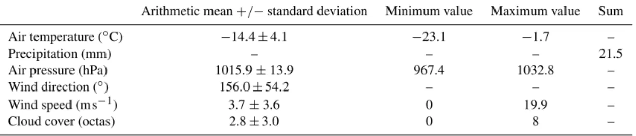
Table 1.Meteorological average conditions during the water sampling period (15 February to 7 March 2010) measured at Ny- ˚Alesund and provided by the Norwegian Meteorological Institute.
Arithmetic mean+/−standard deviation Minimum value Maximum value Sum
Air temperature (◦C) −14.4±4.1 −23.1 −1.7 –
Precipitation (mm) – – – 21.5
Air pressure (hPa) 1015.9±13.9 967.4 1032.8 –
Wind direction (◦) 156.0±54.2 – – –
Wind speed (m s−1) 3.7±3.6 0 19.9 –
Cloud cover (octas) 2.8±3.0 0 8 –
so-called “local water” and “winter cooled water” (WCW) are formed in the fjord due to surface cooling and convection (Piehl Harms et al., 2007).
Meteorological average conditions for the period 15 February to 7 March are summarized in Table 1.
2.3 Experimental setup
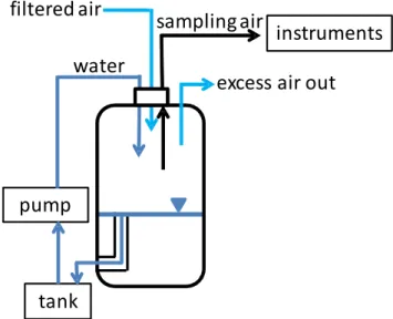
The collected sea water was poured in a storage stainless steel 190 l tank from which it was pumped into a carefully sealed polyethylene bottle (Nalgene Labware) at a rate of 4.8 l min−1 using an aquarium centrifugal pump (EHEIM).
The water entered the bottle through a stainless steel nozzle with an inner diameter of 5 mm producing a water jet mim-icking a falling wave crest which entrains air in sea water. This air subsequently breaks up into bubbles which burst at the water surface. The distance between the nozzle exit and the water surface was approximately 16 cm. The water level in the polyethylene (PET) bottle was kept stable by a sim-ple overflow system and the water volume remained constant at 10 l. Water flowing from the PET bottle was transferred back to the buffer storage tank through a PVC tube (more details about the experimental procedure can be found in Sect. 2.5). During one experiment the water flow was higher than 4.8 l min−1resulting from a lower water pump position
(see end of Sect. 3.2).
Fuentes et al. (2010) compared different mechanisms for marine aerosol production in laboratory experiments with re-spect to their ability to reproduce a realistic oceanic bubble size spectrum. It was concluded that a plunging water jet was best at reproducing the shape of an oceanic bubble size spec-tra (cf. also Hultin et al., 2010). Hence, it is assumed that this method also results in the most realistic bubble-mediated aerosol size spectra (i.e., neglecting spume droplets produced from tearing of breaking waves).
To avoid any contamination by room air, air was pumped through an Ultra Filter (type H cartridge, MSA, Pittsburgh) into the PET bottle at flow rate of 12 l min−1. Excess air of
1 l min−1was allowed to freely leave the top of the PET
bot-tle through an opening of 5 mm in diameter. The quality of the particle-free air and the integrity of the whole setup were regularly checked by switching off the water jet, to confirm that the particle number concentration in the air space of the
PET bottle returned to zero. The sample air was collected from an air volume above the sea water in the PET bottle. The total sampling air flow was kept stable at 5.0 l min−1
dur-ing all experiments. A scheme of the experimental setup is shown in Fig. 2 and parameters and physical characteristics of the bubble tank are listed in Table 2.
2.4 Instrumentation
The air sampling outlet of the PET bottle was connected through a 2 m long 1/4′′ stainless steel tube to the instru-mentation that provided information about aerosol number concentration and size distribution. Based on the geometry of the aerosol sampling lines and associated inertial losses, the upper size limit which was reliably detected was estimated to be around 5 µm in diameter (Dp).
The total aerosol number concentration was measured at 1 Hz for all particles with aDp>0.01 µm using a TSI model
3010 Condensation Particle Counter (CPC) and for all par-ticles with aDp>0.25 µm using a GRIMM 1.109 Optical Particle Counter (OPC).
The size distribution for the size range 0.01 µm< Dp<
0.30 µm was determined using a closed-loop sheath air custom-built differential mobility particle sizer (DMPS) equipped with a TSI 3010 CPC. One scan covering 15 size bins was completed in 2.5 min. The aerosol size distribution in the range 0.25 µm< Dp<32 µm was determined every 6 s
with a GRIMM 1.109 Optical Particle Counter (OPC), siz-ing particles in 31 bins. The relative humidity of the sam-pled air was monitored in the sampling line prior to enter-ing individual instruments with a Hygroclip SC04 hygrome-ter (Rotronic). The relative humidity near the sensing instru-ments was always lower than 10 %, which is mainly a result of the relative high temperature in the instrument payload. Whereas the aerosols were characterized as dry aerosol par-ticles, the relative humidity conditions in the bottle where the bubbles were produced were significantly higher.
Water temperature, salinity, and oxygen saturation were continuously measured in the steel tank with a Stratos 2402 Cond and a Stratos 2402 Oxy from the Knick Elektronische Messger¨ate GmbH & Co.
water
filtered air
tank
pump
instruments
excess air out
sampling air
Fig. 2.Schematic picture of bubble bursting experimental setup. The tank was used as a buffer to recirculate the sea water sample trough the PET bottle, where SSA was produced by an impinging water jet. Darker blue lines represent water, and the triangle symbol indicates the water surface in the bottle.
impinging water jet comparable to the one used to produce aerosols in the PET bottle, was determined using an optical bubble spectrometer (TNO-mini BMS) in the stainless steel tank (Leifer et al., 2003). Similar to previous studies by, for example, Hultin et al. (2010) and Fuentes et al. (2010), the bubble spectrum was measured in a tank separate from the aerosol spectrum due to the size of the BMS and in order to avoid contamination.
2.5 Experimental procedure
Each one of the water samples of 180 l collected at the loca-tions mentioned in Sect. 2.1 was divided into two equal sub-samples. One subsample was used immediately in a bubble bursting experiment, whereas the other subsample was stored in a dark room at 4◦C air temperature (to minimize biologi-cal activity) for later experiments on the following day. The dark room was the only option to store the water at a rela-tively low temperature without freezing. Eliminating the risk of freezing was desired as a subsequent melting would be slow. A long melting time could result in a higher biological activity compared to the activity expected when storing the sample at 4◦C in a dark room.
Two different types of experiments were performed, “warming experiments” where the water was slowly warmed up during the measurements and “cooling experiments” where the water was slowly cooled down. During warming experiments, the complete experimental setup was placed in-side the marine laboratory where the water sample warmed up due to its exposure to room temperature. For the cooling experiments, the sea water sample was first placed indoors
Table 2.Physical characteristics of the bubble bottle.
Parameter Characteristic number
Water volume 10 l
Water flow rate 4.8 l min−1
Distance nozzle to water surface 16 cm
Inner diameter of stainless steel nozzle 5 mm
Air sampling rate 5 l min−1
Turn over time water 2.1 min
Turn over time air 0.8 min
where it warmed up to approximately 6◦C. Thereafter, the buffer tank was placed on a terrace outside the marine labora-tory and exposed to ambient air temperatures around−10◦C to−15◦C, while the rest of the setup and instrumentation remained indoors. The water from the buffer tank was trans-ported into the marine laboratory through an open window slit. The tank was never exposed to direct sunlight.
The average warming and cooling rates were estimated to range between 1 and 2◦C h−1. This warming rate is more
than twice of that measured during a few daily warming events in the Arctic Ocean (up to 0.4◦C h−1, Eastwood et al.,
2011). Given the high warming and cooling rates in the ex-periments, possible biologically-based long-term changes of water chemistry are most likely missed due to the short time frame of the measurements (approx. 6 h).
3 Results
In this section we present the analysis of the influence of water temperature on the air bubble spectrum. Links be-tween SSA microphysical properties (number concentration and size distribution) and the Arctic Ocean water tempera-ture, salinity, and oxygen saturation were analyzed. Medians for the aerosol characteristics were calculated for 1◦C wide Twbins. The total observational time per temperature bin
var-ied between 8 and 73 min during warming experiments and between 6 min and close to 3 h during cooling experiments, respectively. Salinity bin widths were chosen as 1 ‰, with a smaller bin width for salinities lower than 28 ‰ as a result of limited data in this range (the lowest salinity measured was 26.5 ‰ and no salinity with 27.9 ‰ was recorded). The total measurement time for each salinity bin was between 20 min and close to 34 h. Based on the relatively narrow oxygen saturation range between 72 % and 83 %, associated aerosol data were not binned according to oxygen saturation. The typical duration of one experiment was approximately 6 h.
3.1 Air bubble spectra dependence on sea water
temperature
on the influence of water temperature on SSA properties. The influence of different salinities and oxygen saturations on the bubble development could not be sufficiently studied due to a limited number of bubble spectra measurements (varying between one and seven measurements perTw bin). Within
each temperature bin, the oxygen saturation and salinity val-ues covered only a narrow data range.
All recorded bubble spectra were analyzed for the differ-ent water temperatures. In order to obtain a better compar-ison between the bubble spectra at different water temper-atures, the bubble number size distributions were normal-ized to the size distribution at the highest water temperature. Within each size bin, no trend in the air bubble population with water temperature could be detected (data not shown).
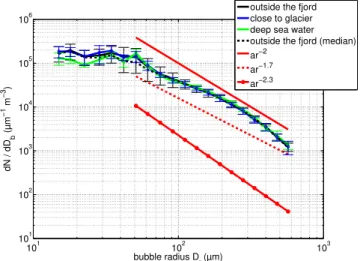
All air bubble spectra were divided according to sampling location and the average concentrations per bubble diameter were calculated (Fig. 3). Figure 3 is based on 28 bubble spec-tra measurements in water sampled outside the fjord, nine measurements in water sampled close to the glacier and five measurements in deep sea water samples. All averaged bub-ble spectra show a similar shape, with one peak atDb70 µm
and one atDb100 µm followed by a steady decrease of
bub-ble number concentration with increasing bubbub-ble diameter. A two-sample Kolmogorov-Smirnov test with a rejection of the null hypothesis at a 5 % significance level was ap-plied to the different bubble spectra. A significant difference was found between the deep and glacier water bubble size distributions for the first three size bins (Db 30 µm, 36 µm
and 45 µm) and for bubble diameters of 84 µm and 465 µm. A comparison of the bubble spectra resulting from water out-side the fjord and the deep water showed significant differ-ences atDb45 µm andDb123 µm.
The shapes of the averaged bubble number size distribu-tions, for the three different waters, were compared to typ-ical bubble size distributions measured in the ocean to en-sure that the preconditions of producing realistically aerosol spectra apply. Generally, bubble size distributions can be de-scribed as a power law function (Bowyer, 2001; Leifer and de Leeuw, 2006; Hultin et al., 2010) with the radius of the bubbler:
dN/dr=ar−b. (1)
For 0.1 mm< Db<1 mm, the exponent b for bubble size
distributions observed in the real ocean has been estimated to be close to 2 (see Hultin et al., 2010, for a compilation of measurements). Power law functions with the exponents of b=2,b=1.7 andb=2.3 are shown in Fig. 3 and suggest that the measured bubble spectra are comparable to bubble spectra occurring in the ocean, at least forDb>0.1 mm. In
addition to the arithmetic mean values of the bubble spectra shown in Fig. 3, a median is shown as an example. For the bubble size range which follows the typical power law func-tion of bubbles in the real ocean (Db>0.1 mm), the
arith-metic mean and the median of the bubble spectra are essen-tially not different. Even at sizesDb<0.1 mm, the difference
101 102 103
101 102 103 104 105 106
dN / dD
b
(µm
−
1 m
−
3)
bubble radius Dr (µm)
outside the fjord close to glacier deep sea water outside the fjord (median) ar−2
ar−1.7 ar−2.3
Fig. 3.Solid lines represent arithmetic means with standard devia-tions for bubble population distribudevia-tions versus bubble diameter for different water sampling locations. The black dashed line shows as an example a median for comparison with the arithmetic mean. Av-erages are based on 28, 9, and 5 bubble spectra measurements from bubbles produced in water with its origin outside the fjord (black line), close to the glacier (blue line) and deep water (green line), re-spectively. Red lines represent power law functions dN/dr=ar−b with the bubble radiusrforb=2,b=1.7 andb=2.3.
is limited to at the most 30 %. For the other water types, the difference is smaller.
3.2 Particle number concentration dependence on
water temperature
The particle number concentrations as a function ofTw
−2 −1 0 1 2 3 4 5 6 7 8 9 100 500
1000 1500 2000 2500 3000 3500 4000 4500 5000
water temperature (°C)
particle number concentration
(particles cm
−
3)
D
p > 0.01 µm
outside the fjord close to glacier deep sea water
−2 −1 0 1 2 3 4 5 6 7 8 9 100 200
400 600 800 1000 1200
D
p > 0.25 µm
water temperature (°C)
particle number concentration
(particles cm
−
3)
outside the fjord close to glacier deep sea water b)
a)
Fig. 4.Medians of particle number concentration for distinct water temperature bins and each experiment. Dashed lines represent 25th and 75th percentiles. The salinity was between 34.3 and 34.4 ‰ for the sampled water close to the glacier, 34.4 to 34.7 ‰ for the deep water and 34.1 to 35.0 ‰ for experiments which were con-ducted using sea water from outside the fjord.(a)Measurements for particles withDp>0.01 µm.(b)Measurements for particles with
Dp>0.25 µm. Note the different scales.
of WCW occurring in Kongsfjorden is approximately be-tween 34 ‰ and 35 ‰ (Piehl Harms et al., 2007). For the to-tal particle number concentration, particle sizes are analyzed separately forDp>0.01 µm andDp>0.25 µm based on the
cut-off sizes of CPC and OPC used for the measurements. Generally, particle number concentrations decrease with increasing water temperature. This effect is clearest for the lowest water temperatures, while for higher temperatures the decrease levels off. The magnitude of this effect is differ-ent for the differdiffer-ent water samples (Fig. 4). Quantitatively, the surface water from the fjord mouth spans a wider range of particle number concentrations (up to a factor of 5) for a given temperature compared to particle concentrations re-sulting from deep sea water and water close to the glacier. The water sampled close to the glacier results in one curve close to the center of the data range and one in the upper range from the fjord mouth water, while both curves resulting from deep water are in the upper range (Fig. 4). We cannot say, however, if additional experiments would have shown a larger variation for the glacier and deep water, as well. For the glacier water, where we have two experiments, the tem-perature range shows a difference in particle number con-centrations of up to a factor of about 2–3 (forTw between
4 and 5◦C andD
p>0.01 µm). At sea water temperatures of
around 6◦C–7◦C, the particle number concentrations gener-ally converge to around 400 particles cm−3(D
p>0.01 µm)
and 200 particles cm−3(D
p>0.25 µm) (Fig. 4a, b).
As previously described, half of the sea water sample was used on the same day the sample was collected and the
sec-−2 −1 0 1 2 3 4 5 6 7 8 9 100 500
1000 1500 2000 2500 3000 3500 4000 4500 5000
water temperature (°C)
particle number concentration
(particles cm
−
3)
D
p > 0.01 µm
outside the fjord close to glacier deep sea water
−2 −1 0 1 2 3 4 5 6 7 8 9 100 200
400 600 800 1000 1200
water temperature (°C)
particle number concentration
(particles cm
−
3)
D
p > 0.25 µm
outside the fjord close to glacier deep sea water
a) b)
Fig. 5. Medians of the particle number concentration as a func-tion of water temperature for different sampling locafunc-tions. Dashed lines represent the 25th and 75th percentiles.(a)Measurements for particles withDp>0.01 µm.(b)Measurements for particles with
Dp>0.25 µm. Note the different scales.
ond half was used in an identical experiment the subsequent day (though not always covering exactly the same tempera-ture range). The experiments from the first day were com-pared with the experiments from the second day for the dif-ferent types of water. The smallest difference was obtained for deep sea water (not shown), where the particle number concentrations differed by less than 10 % (Dp>0.01 µm)
and around 7 % (Dp>0.25 µm). For the water sample
col-lected close to the glacier, the particle number concentra-tions were 44 % lower (Dp>0.01 µm) in the experiment
conducted the first day compared to the second day, and 51 % lower for particles with aDp>0.25 µm. For the surface
wa-ter from the fjord mouth, the particle number concentration for the first experiment was on average 97 % and 68 % lower for particlesDp>0.01 µm and particles Dp>0.25 µm,
re-spectively. Comparing the other two experiments replicated with sea water outside Kongsfjorden resulted in differences around 14 % for both particles withDp>0.01 µm and
parti-cles withDp>0.25 µm.
Medians of the particle number concentrations for each water temperature bin for the distinct water types are shown in Fig. 5. The median of the particle number concentra-tions for the different water types converge at Tw>6◦C.
Figure 5 indicates that belowTw 7◦C, the median particle
number concentrations (for particles with a Dp>0.01 µm
and particlesDp>0.25 µm) produced from the water
−0.05 0 0.05 0.1 0.15 0.2 0.25 0.3 0.35 D
p > 0.01 µm outside the fjordclose to glacier
deep sea water
−0.05 0 0.05 0.1 0.15 0.2 0.25 0.3 0.35 temperature bins
particle number concentration change (−)
D
p > 0.25 µm outside the fjordclose to glacier
deep sea water
−1.5 °C to −0.5 °C −0.5 °C to 0.5 °C 0.5 °C to 1.5 °C 0.5 °C to 1.5 °C 1.5 °C to 2.5 °C −0.5 °C to 0.5 °C 1.5 °C to 2.5 °C 2.5 °C to 3.5 °C 3.5 °C to 4.5 °C 4.5 °C to 5.5 °C 4.5 °C to 5.5 °C 5.5 °C to 6.5 °C 6.5 °C to 7.5 °C 7.5 °C to 8.5 °C 7.5 °C to 8.5 °C 8.5 °C to 9.5 °C 8.5 °C to 9.5 °C a) b) 2.5 °C to 3.5 °C 3.5 °C to 4.5 °C 5.5 °C to 6.5 °C 6.5 °C to 7.5 °C −1.5 °C to −0.5 °C
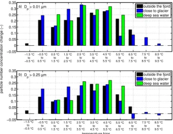
Fig. 6.Medians of the relative change in particle number concentra-tion from one temperature bin to the previous one. Numbers on the x-axis represent the middle of the two temperature bins for which the particle number concentration change was calculated.(a) Mea-surements for particles withDp>0.01 µm.(b)Measurements for
particles withDp>0.25 µm.
a significant difference for all waters and temperature bins (significance level of 5 %).
The relative change in aerosol number density from one temperature bin to the next one shows a maximum atTw
be-tween 2◦C and 5◦C (Fig. 6). At this temperature range, the decrease ofTwby one degree results in an increased aerosol
concentration of the order of 22 % to 33 % for particles with Dp>0.01 µm and between 14 % to 27 % for particles with
Dp>0.25 µm, depending on the type of water. At higher and
lower sea water temperatures the rate of change in the aerosol concentration is lower. This type of pattern is observed for all three types of water (Fig. 6), but it is less pronounced for the glacier water.
To test whether the increase in aerosol concentrations with decreasing water temperature is a robust feature and to ex-clude possible unknown experimental artifacts, the whole procedure was performed in a reversed manner. The sec-ond half of the sample was in two cases slowly warmed up in darkness to 2◦C and 5◦C, respectively. The bubble bursting experiment was then carried out, while the tank with sea water was placed on a terrace outside the marine laboratory and the sample water was slowly cooled down by the ambient outside air temperature (approx. −12◦C). In Fig. 7 the warming experiments (referred to as W1 and W2) with their associated cooling experiments (referred to as C1 and C2) are presented. It is clear that cooling of the sea water from 2◦C (C1) and 5◦C (C2), respectively to sub-zero temperatures resulted in increased particle number con-centrations for both cases, i.e., a mirroring of the warming experiments. For the warming/cooling experiment W2/C2, the change in aerosol emissions with sea water
tempera-−3 −2 −1 0 1 2 3 4 5 6 7 8 9 100 500 1000 1500 2000 2500 3000 3500
water temperature (°C)
particle number concentration (particles cm
−
3)
D
p > 0.01 µm
W1 C1 W2 C2
−3 −2 −1 0 1 2 3 4 5 6 7 8 9 100 100 200 300 400 500 600 700 800 900
water temperature (°C)
particle number concentration (particles cm
−
3)
D
p > 0.25 µm
W1 C1 W2 C2 b) a)
Fig. 7. Comparison of warming experiments with their re-lated cooling experiments using sea water from outside the fjord (W1 = warming experiment 1, C1 = cooling experiment 1, W2 = warming experiment 2, C2 = cooling experiment 2). The same markers indicate two related types of water. Dashed lines are the 25th and 75th percentiles. Red solid lines represent experiments with increasing water temperature and blue solid lines experiments with decreasing water temperature.(a)Medians of particle number concentration withDp>0.01 µm.(b)Medians of particle number concentration withDp>0.25 µm.
ture shows a similar trend of comparable magnitude. The aerosol number density forDp>0.01 µm changed by 87 %
(C2) and 89 % (W2) for a change betweenTw=0.5◦C and
Tw=5.6◦C. The associated accumulation mode aerosol
den-sity forDp>0.25 µm changed by 82 % (C2) and 81 % (W2),
respectively. The other set of warming/cooling experiments (W1/C1) displayed a similar trend, but with much larger dif-ference in magnitude between the cooling and warming ex-periments. The number particle concentration change was 51 % for C1 and 35 % for W1 with Dp>0.01 µm (from
Tw= −0.5◦C toTw=1.5◦C). A number increase of 35 %
(C1) and a decrease of 24 % (W1) were calculated for parti-cles withDp>0.25 µm.
Table 3.Salinity bins and the days from which the median total particle number concentration for the different water temperature bins was calculated.
Salinity bin (‰) Day of experiment
26 to 27 7 Mar
27 to 28 7 Mar
32 to 33 5 and 6 Mar
33 to 34 5 and 6 Mar
34 to 35 21, 22, 23, 24, 25, 26, 27 Feb and 1, 5 and 6 Mar
35 to 36 21, 22, 23, 24 Feb and 1, 5 and 6 Mar
3.3 Particle number concentration dependence on
salinity
Besides water temperature, changes in salinity are expected to have a pronounced effect on the aerosol concentration resulting from the bubble bursting process. In the follow-ing subsection, results from experiments coverfollow-ing a salinity range between 26 ‰ and 36 ‰ and measurement times per salinity bin between 20 min and 33 h are presented. Differ-ences in salinity result from
– different sampling locations,
– formation of ice slush at subzero temperatures, and
– adding fresh glacier ice to the water sample.
Fresh glacier ice was collected close to Ny- ˚Alesund and added to a water sample in an attempt to investigate the effect of melted glacier water on aerosol emissions from sea water. Table 3 displays the different salinities and the days the ex-periments were conducted. On the evening of 6 March, fresh glacier ice was added to the water sample and the salinity decreased below 28 ‰ the following day.
On 5 March water was sampled outside the fjord and the salinity was typically expected to be above 34 ‰. However, since the sea was almost completely frozen, except at some spots from where the sampling took place, a high amount of ice slush with a lower salinity was also collected from the ocean surface, leading to relatively low salinities in the sample, i.e., between 32 ‰ and 34 ‰. For all sampling sites, the sea water samples often froze during the transport to the marine laboratory. Therefore, at water temperatures be-tween zero degrees and the freezing point of sea water (about −1.5◦C to−1.9◦C depending on salinity) salinities higher than 34 ‰ were measured as a result of a not yet completely melted sample in the storage tank.
Measured median, 25- and 75-percentile particle number concentrations as a function of water temperature and salin-ity are shown in Fig. 8. ForTw from−2◦C to +2◦C, the
median particle number concentration (Dp>0.01 µm)
de-creases with salinity for each temperature bin, but the vari-ability of particle number concentration within one water temperature bin is, with an interquartile range up to more
−2 −1 0 1 2 3 4 5 6 7 8 9 100 500
1000 1500 2000 2500 3000 3500
water temperature (°C)
particle number concentration (particles cm
−
3)
D
p > 0.01 µm
26 to 27 ‰ 27 to 28 ‰ 32 to 33 ‰ 33 to 34 ‰ 34 to 35 ‰ 35 to 36 ‰
−2 −1 0 1 2 3 4 5 6 7 8 9 100 100
200 300 400 500 600 700 800 900 1000
water temperature (°C)
particle number concentration (particles cm
−
3)
D
p > 0.25 µm
26 to 27 ‰ 27 to 28 ‰ 32 to 33 ‰ 33 to 34 ‰ 34 to 35 ‰ 35 to 36 ‰ b)
a)
Fig. 8.Median particle number concentration dependence of salin-ity for different water temperature bins. Dashed lines represent 25th and 75th percentiles.(a)Medians of total particle number concen-trations for particles with aDp>0.01 µm.(b)Medians of total
par-ticle number concentrations for parpar-ticles with aDp>0.25 µm.
than 1000 cm−3, rather high. As discussed earlier, the aerosol
concentration can vary substantially among individual sam-ples for the same salinity and temperature. The low variabil-ity in measured particle number concentrations for salinities between 32 ‰ and 33 ‰ is likely a result of the small num-ber of experiments conducted for this salinity range (n=1). ForTw from 2◦C to 4◦C, the median particle number con-centration (Dp>0.01 µm) is highest for salinities between
34 ‰ and 35 ‰ and then decreases with decreasing salinity. For higher water temperatures, there is no clear trend of the median particle number concentration with salinity. A simi-lar pattern can be observed for the measurements of particles withDp>0.25 µm.
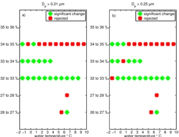
Since the variability of the measured particle number con-centration for a certain salinity within one temperature bin is relatively large, especially for salinities between 33 ‰ and 36 ‰, a two-sample Kolmogorov-Smirnov test was applied to the data. A test was conducted to determine if the particle number concentration of a given salinity within oneTwbin
was significantly lower compared to the particle number con-centration resulting from water having the adjacent higher salinity range. The test was applied for particle number con-centrations withDp>0.01 µm andDp>0.25 µm. Figure 9
shows, that for particles with a Dp>0.01 µm, the
hypoth-esis was fulfilled for salinities between 32 ‰ to 34 ‰ for the whole temperature range and that it was rejected for the salinity range between 34 ‰ and 35 ‰ for Tw>2◦C.
The test results differ only slightly for the particles with a Dp>0.25 µm.
Only in the range of Tw between−2 and −1◦C andTw
−2 −1 0 1 2 3 4 5 6 7 8 9 10 26 to 27 ‰
27 to 28 ‰ 32 to 33 ‰ 33 to 34 ‰ 34 to 35 ‰ 35 to 36 ‰
water temperature ° C D
p > 0.01 µm
significant change rejected
−2 −1 0 1 2 3 4 5 6 7 8 9 10 26 to 27 ‰
27 to 28 ‰ 32 to 33 ‰ 33 to 34 ‰ 34 to 35 ‰ 35 to 36 ‰
D
p > 0.25 µm
water temperature ° C significant change rejected b)
a)
Fig. 9.Green markers show significantly lower particle number concentrations for the salinity to the left of the markers compared to the adjacent higher salinity bin by applying the two-sample Kolmogorov-Smirnov test. The red markers show a rejection of the hypothesis.(a)Dp>0.01 µm(b)Dp>0.25 µm.
number concentrations (for Dp>0.01 µm) between one
salinity bin and the adjacent higher salinity bin, indicating that the particle number concentration followed a trend with salinity. For particles withDp>0.25 µm this was only
ob-served forTwbetween−1 and 0◦C (Fig. 9).
3.4 Particle number concentration dependence on
oxygen saturation
The oxygen saturation in the experiments varied over a nar-row range between 72 % and 83 % during the whole win-ter experiment, which made it difficult to assess a possible influence of oxygen saturation on sea spray aerosol emis-sions. Taking two rather different cases with water temper-ature ranges between 5◦C and 6◦C and 1◦C and 2◦C and similar salinities between 34 ‰ and 35 ‰; a dependence of oxygen saturation on particle number concentration for par-ticles with aDp>0.01 µm andDp>0.25 µm was not
ob-served.
3.5 Influence of salinity on the particle number size
distribution
The influence of salinity on the shape of the particle num-ber size distribution was examined for waters having a water temperature between 6◦C and 7◦C. This temperature range was chosen as the measurements in this interval covered a broad range of salinities (between 26 ‰ and 36 ‰). Me-dian number size distributions for the lowermost measured salinities (between 26 ‰ and 28 ‰) were compared to the size distribution of the highest measured salinities (between
35 ‰ and 36 ‰) and to the most common salinity of 34 ‰ to 35 ‰ (not shown).
All size distributions showed local maxima and minima at the same sizes and no influence of the examined salinity range on the shape of the size distribution was detected. No salinity dependent trend in total particle number concentra-tion for sub-micron and super-micron particles was observed.
3.6 Influence of water temperature on the particle
number size distribution
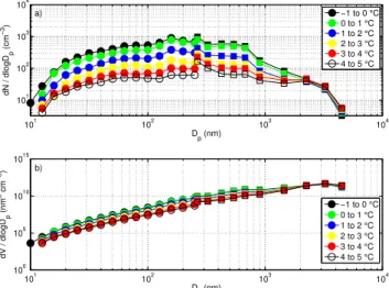
The impact of the water temperature on the magnitude and shape of the aerosol number size distribution was examined using data from measurements performed on 3 and 4 March 2010. The changes in median aerosol size distribution were studied during a warming experiment fromTw−1◦C to 5◦C (Fig. 10) and the corresponding cooling experiment fromTw 4◦C to −2◦C (Fig. 11). These two experiments cover the most relevant sea water temperature range and can be directly compared to each other as they were made with the same wa-ter sample. Aerosol size distributions from other experiments were analyzed in a similar way and the result from these ex-periments are well represented by the example exex-periments from 3 and 4 March (Figs. 10 and 11). For every 1◦C sea water temperature bin, the median aerosol size distribution is based on 8–18 (individual) DMPS size distributions and 150–400 (size) distributions measured by the OPC.
A comparison between the number size distributions re-sulting from warming (Fig. 10a) and cooling (Fig. 11a) shows that for all size distributions, independent of the as-sociated water temperature, there are two local maxima at 180 nm and 570 nm. The most prominent feature is the ro-bustness of the aerosol size distribution shape. Changes re-lated to sea water temperature are pronounced almost only in the magnitude of the aerosol size distribution. The rela-tive proportion between both modes at 180 nm and 570 nm is however changing slightly depending on sea water tem-perature. During both the warming and the cooling exper-iment (Figs. 10a and 11a), for water temperatures up to 3◦C, the maximum at 180 nm is most distinct. For sea water temperatures greater than 3◦C, the peak at about 570 nm is more pronounced. In addition, a smaller local max-imum at around 2 µm becomes more important at higher sea water temperatures. Median aerosol volume size distribu-tions for the same warming and cooling experiments were calculated for the different temperature ranges and are shown in Figs. 10b and 11b. A maximum of the total aerosol volume within the measured size range was observed at dry diame-ters between 3 µm and 4 µm. Below 2 µm size, the aerosol volume is decreasing with increasing sea water temperature in a similar pattern as the aerosol number size distribution.
101 102 103 104 101
102 103 104
dN / dlogD
p
(cm
−
3)
D
p (nm)
−1 to 0 °C 0 to 1 °C 1 to 2 °C 2 to 3 °C 3 to 4 °C 4 to 5 °C
101 102 103 104 100
105 1010 1015
D
p (nm)
dV / dlogD
p
(nm
3 cm
−
3)
−1 to 0 °C 0 to 1 °C 1 to 2 °C 2 to 3 °C 3 to 4 °C 4 to 5 °C a)
b)
Fig. 10. (a)Median particle number size distributions for different water temperatures.(b)Particle volume size distributions for dif-ferent water temperatures. The warming experiment was conducted with water sampled outside the fjord on 3 March 2010. The part of the size distribution measured by DMPS is marked with circles, whereas the part measured by OPC is marked with squares. Only every second bin data point is shown for clarity.
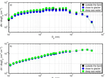
maxima and minima (Fig. 12a). Medians were calculated using between 24–66 size distributions from DMPS mea-surements and between 610–1690 size distributions from the OPC measurements. Peaks in the size distributions are found at about 180 nm, between 375 nm and 615 nm, and around 1.8 µm. The peak at 180 nm and the peak between 375 nm and 615 nm have the same magnitude for each size distri-bution of the different types of water, whereas the mode at 1.8 µm is much lower in magnitude for all size distributions. The slight difference in the magnitude of the peak between the different types of water may result from the large vari-ability in particle number concentration between the experi-ments (Fig. 4). The corresponding volume size distributions for respective types of water (Fig. 12b) show a peak at dry diameters between 3 µm and 4 µm.
4 Discussion
The hypothesis, that primary marine sea spray aerosol emis-sions are affected by changed physical properties of the Arc-tic Ocean, is partly confirmed and partly repudiated. The hy-pothesis was repudiated for a change in oxygen saturation between 72 % and 83 % and could not be confirmed for a change of salinity between 36 ‰ and 26 ‰ (for a wide range of different water temperatures). The hypothesis that an in-crease in average water temperature impacts on SSA emis-sions was on the other hand confirmed. The results which led to these conclusions will be discussed separately for the dif-ferent tested parameters in the following sections, beginning
101 102 103 104 101
102
103 104
D
p (nm)
dN / dlogD
p
(cm
−
3)
4 to 3 °C 3 to 2 °C 2 to 1 °C 1 to 0 °C 0 to −1 °C −1 to −2 °C
101 102 103 104
100
105 1010 1015
D
p (nm)
dV / dlogD
p
(nm
3 cm
−
3)
4 to 3 °C 3 to 2 °C 2 to 1 °C 1 to 0 °C 0 to −1 °C −1 to −2 °C b)
a)
Fig. 11. (a)Median particle number size distributions for different water temperatures.(b)Particle volume size distributions for dif-ferent water temperatures. The cooling experiment was conducted with water which was sampled outside the fjord 3 March 2010 and then stored in a dark room with an air temperature of 4◦C. The part of the size distribution measured by DMPS is marked with circles, whereas the part measured by OPC is marked with squares. Only every second bin data point is shown for clarity.
with a discussion of the results regarding how water temper-ature influenced the air bubble spectra. An influence of water temperature on air bubble spectra was not included in the hy-pothesis, but was expected to give an explanation for possible observed relationships between the tested physical properties and the SSA emissions.
4.1 Effect of sea water temperature on air bubble
number spectra
The observed bubble spectra between about 100 µm< Db<
1140 µm was shown to be comparable to bubble spectra mea-sured during other in-situ experiments under non-laboratory conditions. Consequently, the generated SSA should mimic the bubble driven flux as far as our understanding permits. However, for the experiments presented here, no dependence of the bubble number size distribution on sea water temper-ature was detected for bubbles with 30 µm< Db<1140 µm.
This undetected impact of sea water temperature on the bub-ble spectra is somewhat unexpected since several previous studies have detected such an influence, both in fresh water and in sea water (Hwang et al., 1991; Thorpe et al., 1992; Slauenwhite and Johnson, 1999). Hwang et al. (1991), using an impinging water jet, showed that the entrainment depth of bubbles with a diameter of 0.1 mm increased with increasing water temperatures from 11◦C to about 19◦C and remained at a plateau value for higher water temperatures.
101 102 103 104 100
102
104
D
p (nm)
dN / dlogD
p
(cm
−
3)
outside the fjord close to glacier deep sea water
101 102 103 104 100
105 1010 1015
D
p (nm)
dV / dlogD
p
(nm
3 cm
−
3)
outside the fjord close to glacier deep sea water a)
b)
Fig. 12. (a) Comparison of median particle number size distri-butions for different sea water types.(b) Comparison of median particle volume size distributions. Dashed lines represent the 25th and 75th percentiles. The part of the size distribution measured by DMPS is marked with circles, whereas the part measured by OPC is marked with squares. Only every second data point is shown for clarity.
the viscosity and the solubility of oxygen and nitrogen de-crease. The decrease in viscosity for higher water temper-atures results in a higher bubble rise velocity. At the same time, the reduced solubility of oxygen and nitrogen with in-creasing water temperature leads to an increase of bubble numbers, but this effect is to some extent buffered by the increase in diffusivity. As a net effect, the numerical model by Thorpe et al. (1992) showed an exponential decrease of the mean bubble concentration with increasing temperature, with a halving for every 10◦C for bubbles with radii be-tween about 10 µm and 150 µm at 4 m depth. Since the trans-fer function between bubble number concentration and parti-cle number concentration is unknown, one can only speculate what this implies for our observations.
Our measurements focused on sub-micrometer particles. These particles are most likely a consequence of evaporation and production of so-called film drops with radii between about 10 nm and a few hundred micrometers. Somewhat counter-intuitively, these small droplets (and thus the sub-micrometer particles) are most likely produced by air bub-bles larger than 2 mm in diameter, whereas air bubbub-bles with a radius smaller than 1 mm mainly form droplets with a ra-dius in the super-micrometer range (de Leeuw et al., 2011). With our instrumentation, we could only measure air bubbles withDb<1140 µm. Thus, we could not obtain any
informa-tion regarding the temperature dependence of the bubble size range that was perhaps the most relevant for the particles ob-served.
4.2 Effect of oxygen saturation on particle number
concentration
No dependence of the particle number concentration on oxy-gen saturation between 72 % and 83 % for particles with a Dp>0.01 µm or Dp>0.25 µm was observed. Hultin et al.
(2010) did find a relationship between dissolved oxygen (in an oxygen saturation range between 90 % and 107 %) and sea spray production in the northeast Atlantic Ocean. Hultin et al. (2011) observed an anti-correlation between particle produc-tion and dissolved oxygen at shallow water in the Baltic Sea, following the biologically driven diurnal cycle in the water (oxygen saturation range between 90 % and 100 %).
4.3 Effect of salinity on particle number concentration
The influence of salinities between 26 ‰ and 36 ‰ on the shape and magnitude of the median particle number size dis-tributions revealed no clear trend for water temperatures be-tween 6 and 7◦C. A trend of increasing total particle num-ber concentration with increasing salinity was only observed forTw between−2 and−1◦C andTw between 0 and 1◦C
(both forDp>0.01 µm) and for Tw between−1 and 0◦C
(Dp>0.25 µm). An impact of salinity on particle number
size distribution and particle number concentration has been observed in other studies (M˚artensson et al., 2003; Hultin et al., 2011). M˚artensson et al. (2003) compared number size distributions with salinities of 9.3 ‰ and 33 ‰. Higher num-ber concentrations for particles withDp>0.2 µm, but a simi-lar shape of the distribution, was measured for the water with higher salinity. Hultin et al. (2011) observed higher particle number concentrations over the whole measurement range for higher salinity ranges (examining real ocean water with salinities about 6 ‰, 7 ‰ and 35 ‰ salinity).
4.4 Effect of sea water temperature on particle number
concentration
A dependence of primary marine particle number concen-tration with water temperature has previously been observed by a number of authors (Bowyer et al., 1990; Hultin et al., 2011; Sellegri et al., 2006; M˚artensson et al., 2003). Bowyer et al. (1990) used a 3 m long white cap simulation tank, in which two waves of collected coastal water broke against each other in the middle of the tank. They observed (sim-ilar to our study) a steep decrease of particle number con-centration for particles with a Dp<3 µm with slowly
in-creasing water temperature from 0◦C to 13◦C. For tem-peratures higher than 13◦C, the particle number concentra-tion remained constant. M˚artensson et al. (2003) observed a decrease of particle number concentration with increas-ing water temperatures (for the temperatures −2◦C, 5◦C, 15◦C and 23◦C) for particles withD
p<70 nm. For particles
withDp>350 nm an increase of particle number
of modes from 110 nm to 85 nm, from 45 nm to 30 nm and from 300 nm to 200 nm, when water temperature decreased from 23◦C to 4◦C. Both M˚artensson et al. (2003) and Selle-gri et al. (2006) used artificial sea water and a sintered glass filter at the bottom of an experimental tank to produce the bubbles. Hultin et al. (2011) observed, during experiments with Baltic Sea water, a decrease of aerosol number concen-tration in the size range 0.02 µm< Dp<1.8 µm, when water
temperature of 4◦C changed to 14◦C. The negative correla-tion of the number concentracorrela-tion with water temperature was observed for all particle sizes. An identical setup to the one used in our experiment was used in that study. We conclude that the observed trend of particle number concentration with water temperature is not due to changes of oxygen saturation. This conclusion is based on the fact that a change in oxygen saturation between 72 % and 83 % for the water temperature range 5–6◦C and 1–2◦C did not cause any change in particle number concentration, whereas a change in water tempera-ture within these small intervals did.
Although several studies support our results of a decrease in total particle number concentration with an increase in water temperature (see studies mentioned above), there are some studies indicating the opposite relationship. Monahan and O’Muircheartaigh (1986) demonstrated that for a con-stant wind speed, an increase in water temperature enlarges the whitecap fraction on the ocean surface. This is important, as the sea spray aerosol production is considered proportional to the whitecap fraction. Jaegl´e et al. (2011) compared glob-ally modeled and observed mass concentrations of coarse mode sea salt aerosol (in their study taken to be particles with a radius between 0.3 and 3 µm) and concluded that the modeled bias was improved when introducing an increased sea salt production with increasing water temperature. The increase of whitecap fraction with an increase in surface wa-ter temperature can be explained by an increased production of smaller air bubbles with slower terminal rise velocities compared to larger bubbles with an increase in water temper-ature. Monahan (1985, in Monahan and O’Muircheartaigh, 1986) showed that the time constant characterizing the decay of whitecaps changed inversely with the terminal rise speed of the smaller bubbles. Anguelova et al. (2006) stated that a decrease in viscosity caused by higher water temperatures facilitated wave breaking and as a consequence prolongs the lifetime of a whitecap. Another suggested explanation for ob-served large-scale increases in whitecap fraction with an in-crease in water temperature is the difference in the duration of a certain wind speed over different areas. Trade winds, for example, occur over relatively warm waters and persist relatively long so that whitecaps can fully develop, whereas over colder waters the duration of high wind speeds is rela-tively short (Monahan and O’Muircheartaigh, 1986). During our laboratory experiments, we did indeed produce small ar-eas of whitecaps as a consequence of air bubbles reaching the water surface. However, we did not observe any increase in particle number concentration with an increase in water
temperature, as one would expect if the whitecap fraction de-pends on the sea surface temperature as suggested by Mon-ahan and O’Muircheartaigh (1986) and Jaegl´e et al. (2011). One explanation could be that the water surface in the ex-perimental bottle was too limited to allow for an undisturbed whitecap fraction evolution (that wall effects limited the bub-ble plume and hence the white cap size). On the other hand, no change in the bubble spectrum with temperature was ob-served either, which is notable as this should be a major cause of the whitecap fraction change with water temperature. An-other possible reason for the contradictory results obtained in our study and the ones presented by Jaegl´e et al. (2011) could be that the latter focused on coarse mode concentrations of sea salt, whereas the temperature dependence observed in our study was most clear for aerosols with a diameter smaller than 1 µm. A positive temperature trend could also be ex-plained by the results of M˚artensson et al. (2003), which in contrast to the current study saw increasing aerosol numbers produced at diameters larger than about 350 nm with increas-ing temperature (and decreasincreas-ing numbers for smaller parti-cles in agreement with the current study).
Conducting warming experiments with water sampled at the same time but used on two different days showed parti-cle number concentration differences of up to 97 % (for the same size range and water temperature). The inevitable dif-ferences in experimental setup between the different experi-ments made it difficult to repeat a certain experiment and ob-tain exactly the same results. However, it cannot be excluded that biological and chemical activity modified the properties of the water during storage which may have affected the par-ticle concentration.
In recent years, it has been shown that organic matter may contribute to a large fraction of the SSA sub-micrometer mass (O’Dowd et al., 2004; Vignati et al., 2010). One pos-sible explanation for the observed change in SSA concentra-tion with temperature is that over time, a depleconcentra-tion of organic compounds from the sea water in the storage tank occurred. Even in the beginning of the twilight period in the Arctic, a certain amount of organic material can be expected. Since the polar night near Kongsfjorden lasts from 25 October to 17 February (Svendsen et al., 2002), our measurements took place in the beginning of the biologically active period.
However, our observations, and especially the sets of mir-roring warming/cooling experiments, support that for win-ter Arctic Ocean seawawin-ter, most of the variation in particle number concentration originated from sea water temperature changes and not from a depletion of organic substances from the sea water.
testing and has to be experimentally explored as other stud-ies have shown a clear effect of organic matter on physical properties of water which may alter air bubble generation. For example, N¨ageli and Schanz (1991) reported that surface tension was reduced by phytoplankton exudates and Lion and Leckie (1981) theoretically described the decrease of sur-face tension caused by sursur-face-active organics. An impact of organics on bubble properties was determined by Garrett (1967). A stabilization of air bubbles on the air–sea interface due to surface-active substances scavenged by the air bub-ble while rising to the water surface was observed. However, with our current data, we cannot address the role of surfac-tants in SSA emissions for winter Arctic Ocean conditions. These somewhat contradicting results call for further studies on the role of organic matter on particles emissions from the oceans.
5 Future implication
The observed trend of decreasing SSA production with in-creasing water temperature may have large implications for the climate in the Arctic region. The diminishing sea ice will result in a decreased surface albedo and contribute to a positive feedback of the Arctic warming. At the same time, larger areas of ice-free ocean will provide large areas of po-tential SSA emissions, which in turn can act as a negative feedback by increasing aerosol scattering and by modifying cloud microphysical properties providing additional CCN (cf. Struthers et al., 2011). On the other hand, with increas-ing sea water temperature and as shown in this study, the sea spray source strength might decrease and thus weaken the negative feedback of SSA on Arctic climate. Another impor-tant factor influencing the sea spray aerosol emissions is the wind speed. In order to answer questions about how changes in SSA emissions influence the future Arctic climate, it is important to consider all of the above-mentioned factors. To summarize, there are a number of potential feedback pro-cesses between a future changing climate, changes in surface albedo and changes in sea spray production, for example:
– Increasing (decreasing) water temperature will decrease (increase) sea spray emissions due to changes in the physical properties of water (present study; Bowyer et al., 1990; Hultin et al., 2011).
– Increasing (decreasing) wind velocities will result in in-creased (dein-creased) sea spray emissions (Lovett, 1978; Nilsson et al., 2001; Geever et al., 2005).
– Increasing (decreasing) water temperature will increase (decrease) whitecap fraction and increase (decrease) sea spray emissions (Monahan and O’Muircheartaigh, 1986).
– Increasing (decreasing) wind speed will increase crease) whitecap fraction and thereby increase (de-crease) albedo (Monahan and O’Muircheartaigh, 1986).
– Increasing (decreasing) temperature will decrease (in-crease) sea ice cover and increase (de(in-crease) sea salt emissions (e.g., Nilsson et al., 2001; Struthers et al., 2011).
– Increasing (decreasing) temperature will decrease (in-crease) sea ice cover and decrease (in(in-crease) surface albedo.
Struthers et al. (2011), however, indicated that the impact of future changes in wind speed on the sea salt aerosol produc-tion over the Arctic Ocean was small compared to those as-sociated with changes in sea ice coverage and sea surface temperature. All in all, the magnitude and interplay between the decrease of sea ice coverage, the increasing sea water temperature, changes in wind speed and the possible accom-panied change in whitecap coverage should be addressed in large-scale model studies, where changes in meteorology, ocean characteristics and marine aerosol emissions all are represented in a consistent manner. An updated sea spray aerosol emission parameterization, which better represents the effects of low sea water temperatures on the SSA emis-sion strength, would be useful to develop for these types of studies.
6 Summary and conclusions
The influence of water temperature, salinity, and oxygen sat-uration on sea spray aerosol emissions from winter Arctic Ocean sea water was studied by means of laboratory ex-periments at Ny- ˚Alesund, Svalbard. In ambient conditions, wind speed is the dominant physical parameter determin-ing sea spray production (e.g., Nilsson et al., 2001). Tank experiments, such as those presented in this study, remove any influence of wind speed. The results show that in the absence of wind, sea water temperature is the most impor-tant of the studied parameters controlling the magnitude of sea spray aerosol emissions. During the bubble bursting lab-oratory experiments and for the measured water temperature range between 9◦C and−2◦C, particle number concentra-tions were increasing with a decrease in water temperature. The largest change of magnitude was observed between 2◦C and 5◦C where the rate of change was between 22 % and 33 % per 1◦C for particlesD
p>0.01 µm and between 14 %
and 27 % for particlesDp>0.25 µm. No clear relation was