Using a Simplified Analytical Method
Ivan Martı´nez-Forero1, Antonio Pela´ez-Lo´pez1, Pablo Villoslada2*
1Department of Physics and Applied Mathematics, University of Navarra, Pamplona, Spain,2Hospital Clinic, Institute of Biomedical Research August Pi Sunyer (IDIBAPS), Barcelona, Spain
Abstract
Chemical reaction networks (CRNs) are susceptible to mathematical modelling. The dynamic behavior of CRNs can be investigated by solving the polynomial equations derived from its structure. However, simple CRN give rise to non-linear polynomials that are difficult to resolve. Here we propose a procedure to locate the steady states of CRNs from a formula derived through algebraic geometry methods. We have applied this procedure to define the steady states of a classic CRN that exhibits instability, and to a model of programmed cell death.
Citation:Martı´nez-Forero I, Pela´ez-Lo´pez A, Villoslada P (2010) Steady State Detection of Chemical Reaction Networks Using a Simplified Analytical Method. PLoS ONE 5(6): e10823. doi:10.1371/journal.pone.0010823
Editor:Dov J. Stekel, University of Nottingham, United Kingdom
ReceivedFebruary 24, 2010;AcceptedMay 6, 2010;PublishedJune 3, 2010
Copyright:ß2010 Martı´nez-Foreroet al. This is an open-access article distributed under the terms of the Creative Commons Attribution License, which permits unrestricted use, distribution, and reproduction in any medium, provided the original author and source are credited.
Funding:These authors have no support or funding to report.
Competing Interests:The authors have declared that no competing interests exist.
* E-mail: [email protected]
Introduction
Chemical reaction networks (CRNs) display interesting dynamic properties. In order to understand the temporal evolution of chemical species in reactions, CRN are often modeled through systems involving ordinary differential equations. The ODE system derived from a CRN endowed with mass action kinetics is a polynomial system of several variables. The qualitative behavior of CRNs can be outlined if we can find the stationary solutions to such ODEs. However, most of the time these polynomials are non-linear, making them hard to resolve. In an attempt to circumvent this problem, well known theories have attempted to elucidate the qualititave dynamics of CRNs using methods applied to CRN structure alone (i.e Feinberg’s Chemical Reaction Network Theory and Clarke’s Stoichiometric Network Analysis). Here, we present a theory necessary to understand the dynamic properties of CRNs and accordingly, throughout the text we will follow a classic biochemical reaction network. In 1970, Edelstein proposed a reaction scheme that has multiple steady states and a hysteresis loop [1]. The structure of the model is displayed in Figure 1, whereb the network is composed of three species (A,B and C) and six reactions. The chemical mechanism represented is that of species A autocatalytic production and posterior enzymatic degradation. During the explanation we will assume that chemical reactions occur in a well stirred chemical reactor at constant temperature.
Results
Definitions
A reaction network is composed of three sets [2]:
N
Species: the chemical components of the network;SN
Complexes: the formal combinations of species that appear before and after of reaction arrows;CN
Reactions: specify how complexes are joined by arrows.RIn the Edelstein model S= {A,B,C}, C= {A, 2A, A+B, C,B} and R= {A?2A,2A?A,A+B?C, C?A+B, C?B,B?C}, the number of speciesm, the number of complexesnand the number of reactionsrin the example being dealt with ism~3,n~5and
r~6.
Each chemical entity is associated with a continous variable representing its concentration (measured in moles per litre,M, or in another appropriate unit). Only non-negative concentrations are biologically realistic and we will usexito identify the concentrations of different species. In this way A =x1, B =x2 and C =x3.
Complexes are denotedyand they may be reactant complexes y
or product complexes y’. Reactions are represented as y?y’. A complex vector contains the stoichiometric coefficient of speciesyiin complexy. In open systems we refer to a special complex, known as the zero complex0, for which all entries are 0 and that has as many
entries as the number of species in the system under study. As an
example, the complex vector for complex 2A is
2 0 0 2
4 3
5.
The complex matrix Y is a m6n matrix that contains the complex vectors as columns. A reaction vector is the vector resulting from the subtraction of the reactant complex from the product complex,y’{y. For the reaction A+B?C the reaction
vector is {1
{1 1 2
4 3
5.
The stoichiometric matrix, N, is m6r in size and its columns represent the reaction vectors of the chemical network. For the Edelstein model we obtain
Y~
1 2 1 0 0
0 0 1 0 1
0 0 0 1 0
2
6 4
3
7 5N~
1 {1 {1 1 0 0
0 0 {1 1 1 {1
0 0 1 {1 {1 1
2
6 4
3
In general, chemical networks have conserved relationships that can be identified by calculating the left null space of N. Ifsis the rank of N, there arem{sconserved relationships. Therefore, in our working examples~2, there is a relationship of conservation
x2zx3~c. The conservation relationship gives rise to
stoichio-metric compatibility classes that have important consequences in the study of CRN equilibrium solutions.
The kinetics for a reaction network {S,C,R} involve a function that describes the rate at which the chemical species interact to form products. The most common kinetics implemented so far are mass action kinetics (MA). In MA, the rate of the reaction is proportional to the product of the concentration of the reactant species and a kinetic constantki. The general form of MA is
Ky?y’(x)~ky?y’
P
s[Sxys
s ð2Þ
where x is the concentration vector. In these MA, the reaction parameters are positive, and the are estimated using chemical principles or they are deduced from experiments. It is noteworthy that accurate values for such parameters are not often known for complex chemical networks. The reaction rates form a vector
v[Rr, which in the Edelstein case is v~(k1x1,k2x12,k3x1x2,
k4x3,k5x3,k6x2)t
The matrix N can be viewed as the multiplication of two matrices
YIawhereYis the complex matrix andIais ann6rincidence matrix [2]. Each column ofIarepresents a reaction and has an entry21 for
the reactant complex and 1 for the product complex. Likewise, the reaction vector v is the product of IkY(x). Ik is a r6n matrix containing the rows of the kinetic constants for each reaction,kifor reactants.Y(x)is a monomial vector for the species participating in each complex [3]. For the Edelstein example
Ia~
{1 1 0 0 0 0
1 {1 0 0 0 0
0 0 {1 1 0 0
0 0 1 {1 {1 1
0 0 0 0 1 {1
2 6 6 6 6 6 6 4 3 7 7 7 7 7 7 5
ð3Þ
Ik~
k1 0 0 0 0
0 k2 0 0 0
0 0 k3 0 0
0 0 0 k4 0
0 0 0 k5 0
0 0 0 0 k6
2 6 6 6 6 6 6 6 6 4 3 7 7 7 7 7 7 7 7 5
Y(x)~
x1
x2 1
x1x2
x3 x2 0 B B B B B B @ 1 C C C C C C A
ð4Þ
The ODE system for a chemical network is of the form
_ x
x~Nv(k,x) ð5Þ
where N is the stoichiometric matrix andvis the reaction vector. Using the decomposition previously explained, the ODE system is also presented in the following form
_ x
x~YIaIkY(x) or xx_~YAY(x) ð6Þ
According to these considerations, the differential equations for the Edelstein network are
_ x
x1~k1x1{k2x12{k3x1x2zk4x3
_ x
x2~{k3x1x2zk4x3zk5x3{k6x2
_ x
x3~k3x1x2{k4x3{k5x3zk6x2
ð7Þ
As a final definition is needed. The stoichiometric subspace for a reaction network is the linear subspace defined by
T~span(y’{y[Rr:y?y’[R) ð8Þ
In our example, the stoichiometric subspace is generated by the reaction vectors {C-B,A}. The significance of T is that the concentration of each chemical is constrained to evolve in an defined subspace, which is a parallel translation of T. Stoichiometric compatibility classes are parallel translates of the stoichiometric subspace.
Equilibrium solutions
In the previous section we explained a framework for CRNs. Starting from the structure of chemical reactions, it is possible to derive an ODE system for the dynamical study of CRN in a unique and orderly way. Differential equations obtained from a CRN are tied to the network structure. Thus, from this point on if we know the reaction parameters (with appropriate units) and initial conditions, we can commence a numerical analysis of the systems to determine how the species’ concentrations change over time. If parameters are difficult to obtain, it would be desirable to gain some insight into the dynamic capacities of the CRN using reaction structure alone. This approach has been promoted and called ‘‘complex biology with no parameters’’ [4]. In order to understand a CRN we would like to solve the vectorial equationNv(k,x)~0to determine the stationary states where the system converges. Thus, we are faced with the need to resolve several variables of a non-linear polynomial system. Two general theories have adressed this issue : Feinberg’s Chemical Reaction Network Theory (CRNT) and Clarke’s Stoichio-metric Network Analysis (SNA) [2] [5]. SNA and CRNT are methodologies to study the qualitative dynamic behavior of chemical networks [6]. CRNT has received special attention in recent years as it is a reliable method to rule out hypotheses about the mechanism of a particular CRN [7][8][9][10][11][12]. If other tools (i.e. SNA and CRNT) can identify the possibility of a certain dynamic behavior, the
Figure 1. Edelstein chemical reaction network scheme. X1~A,X2~B,X3~C.
method we explain in the following sections provides an essential tool to determine where this behavior might occur.
Region of multistationarity
In many cases SNA and CRNT can decide whether or not a specific CRN is capable of displaying multistationarity. However, it is still necessary to locate the region where this property might appear, and algebraic geometry methods are a natural choice to address that need. To ilustrate how to use algebraic geometry to reveal the site of multistationarity, we will continue dissecting the Edelstein network. As already mentioned, this network displays multistationarity for certain values of the reaction parameters. Figure 2 shows how according to the different locations of the equilibrium curve and the stoichiometric compatibility class intersections, there may be one, two or even three steady states. In order to identify the exact points of intersection we followed the procedure below:
1. Reduce N to its row reduced echelon form, RD; 2. Identify stoichiometric compatibility classes;
3. Based on the RD construct, new equations are derived by multiplying RD by the vector of reaction ratesv(k,x);
4. Add the equation representing stoichiometric compatibility classes to the previous system (conservation relationships). We will call this new equation system AD;
5. Calculate the Gro¨bner basis of AD using an elimination order (i.e. lexicographic order);
6. Normally, this basis will produce a set of polynomials arranged in echelon form.
The procedure for the Edelstein system yielded the following result:
RD~
1 {1 0 0 {1 1
0 0 1 {1 {1 1
2
6 4
3
7
5 v(k,x)~ k1x1
k2x21
k3x1x2
k4x3
k5x3
k6x2
2
6 6 6 6 6 6 6 6 4
3
7 7 7 7 7 7 7 7 5
x2zx3~c
The new system AD is
k1x1{k2x21{k5x3zk6x2~0 k3x1x2{k4x3{k5x3zk6x2~0
x2zx3{c~0
ð9Þ
Now we can calculate the Gro¨bner basis for the new system.x1
represents the chemical product in the Edelstein network and thus, it is of interest to represent equilibrium solutions ofx1in terms of
the differentcvalues. The MAPLE command to obtain the basis is gbasis([f,g,h],plex(x2,x3,x1,c)), where f,g,h are each of the elements
in the polynomial system AD. The complete basis is a huge polynomial system and therefore, we have not reproduced it here.
Figure 2. Number of equilibrium solutions for the Edelstein system by changing the value of conservation relation.Parameter values arek1~8:5,k2~k3~k4~k5~1,k6~0:2.
Using the parameters described previously [2], the first element of the basis is10x1c{2cz10x13{63x21{187x1. A diagram of the
solution for x1 in terms ofc appears in Figure 3, based on the
formula obtained analytically 10x1c{2cz10x13{63x21{187x1.
It is evident that multistationarity is only possible for a small range ofc. Algebraic geometry methods allowed us to identify in which interval of the stoichiometric compatibility class multiple steady states exist. When correctly applied, the method developed in this section is able to identify the region of multistationarity. We would like to highlight that the procedure remains silent in terms of the local stability of the computed steady states. In order to determine the stability, it is neccesary to calculate the eigenvalues of the Jacobian matrix evaluated at the specified steady state. Below we have used the method described to analyse a mathematical model of apoptosis.
Aplication of Gro¨bner basis for the study of apoptosis Apoptosis is an essential process to maintain homeostasis in organisms. Abnormalities in the control of apoptosis can promote the development of autoimmune diseases, neurodegenerative diseases or cancer. Thus, understanding the apoptosis machinery is of considerable biological and medical interest. Apoptosis is a suitable system for mathematical modeling. First, it is complex, by which we mean that its collective properties cannot be explained from the study of each component in isolation. Second, it displays a qualitative property (bistability) useful to model validation. Third, the central mechanism of apoptosis is well known and the parameters for ODE simulation are available in the literature. In this regard various attempts to model apoptosis have been published [13][14][15].
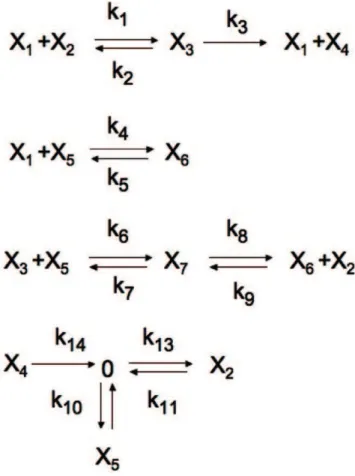
Based on our current knowledge of how apoptosis is regulated, we describe here a new model for receptor induced cell death. The CRN represents Caspase 8 dependent activation of Caspase 3 and inhibition of apoptosis mediated by BAR (Bifunctional Apoptosis Regulator) [16][17]. Figure 4 represents a diagram of the proposed model. The model has seven species and fourteen reactions. The species are:
N
x1= Activated Caspase 8 (C8*)N
x2= Caspase 3 (C3)N
x3= The C8*C3 ComplexN
x4= Activated Caspase 3 (C3*)N
x5= Inhibitor of apoptosis (BAR)N
x6= The C8*BAR ComplexN
x7= The C8*C3BAR ComplexThe reaction rates conform to the vector v~(k1x1x2,k2x3,k3x3,
k4x1x5,k5x1,k6x3x5,k7x7,k8x7,k9x2x6,k10x2,k11x5,k12x4,k13,k14): The ODE system for this network is
_ x
x1~{k1x1x2zk2x3zk3x3{k4x1x5zk5x6
_ x
x2~{k1x1x2zk2x3{k9x2x6{k10x2zk13
_ x
x3~k1x1x2{k2x3{k3x3{k6x3x5zk7x7
_ x
x4~k3x3{k12x4
_ x
x5~{k4x1x5zk5x6{k6x3x5zk7x7{k11x5zk14
_ x
x6~k4x1x5{k5x6zk8x7{k9x2x6
_ x
x7~k6x3x5{k7x7{k8x7zk9x2x6
ð10Þ
There is a conserved relation for total C8* that is represented by
x1zx3zx6zx7~et. We would like to know if our model displays
bistability as required. In order to verify this issue, the parameters
Figure 3. Bifurcation diagram x1 vsc. Parameter values are the same as in Figure 2.
doi:10.1371/journal.pone.0010823.g003
reported for some of the reactions in the apoptosis network were used in a numerical analysis [18] using the procedure explained above. The complete derivation can be followed with a MAPLE file available upon request.
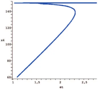
If we use theetconservation relation as a parameter of bifurcation, it is possible in the model now proposed to admit three stady states in a range of total C8*, two stable and one unstable. In Figure 5 the bifurcation diagram for the apoptosis system obtained through the analysis described above is shown. Slight changes in turnover rates influence the dynamic behavior of CRNs and now, we wish to carry out a similar procedure for the apoptosis model proposed. The parameterk11controls the degradation of BAR (x5), an inhibitor of
caspase activation. The bifurcation diagram in Figure 6 shows how even for a region that is supposed to display multistationarity (et~2
according to Figure 5) mild variations ink11 allows the system to
commute between low and high levels of executioner caspase x4
(cleaved caspase 3). This is interesting because if a pharmacological perturbation does not interfere with the total amount of the initiator caspase (Total C8 =et), the system can be controled with drugs that promote or inhibitx5degradation. The clinical implication is if the
physician wants to promote apoptosis (i.e. in cancer cells), a temporary increase shoudl be induced k11, whereas to inhibit
apoptosis he should just prescribek11a transient reduction.
Discussion
In this work we propose a new method to analyse CRNs based on algebraic geometry and we have applied this method to two well known biochemical examples. The method is useful to find the locus of multistationarity in CRNs that display this property in a fully analytical way. Very recently, various groups provided key insights into the application of algebraic geometry to study CRNs [19–20], yet we believe that the procedure developed here stands out due to its simplicity and resolving power. However, the high computational cost underlying the calculation of Gro¨bner basis is a limitation when using algebraic geometry methods. This problem can be overcome by dividing the CRN into subnetworks, resolving each subnetwork and then applying the results to the overall CRN
[21]. We evaluated a model for the mechanisms of apoptosis and instead of a simulation approach, we used an analysis based only on the structure of the reaction network. This parameter-free approximation has gained considerable attention in the field of systems biology [21] [4]. In particular the relation between the structure of the network and the qualitative properties inherent to the system (like bistability) is of great importance due to the difficulty in identifying reliable reaction parameters [22].
Chemical reactions are usually modeled by lumping together reactions and ignoring the behavior of intermediary products. This can lead to different dynamic properties if one compares the behavior of complete mechanisms and their lumped counterpart. For example using CRNT, it was recently shown that a simple model of enzyme catalysis that exhibits multistationarity lost this property by neglecting enzyme-substrate intermediates [23]. Representing chemical reac-tions as accurately as possible is essential when developing appropriate mathematical models of cellular processes.
In summary our results illustrate the power of algebraic geometry methods to evaluate the dynamic capabilities of a chemical reaction network.
Materials and Methods
The ODE system derived from a CRN endowed with mass action kinetics is a polynomial system. Most of the time these polynomials are non-linear, making it difficult to calculate the steady states. During the last few years, there has been growing interest in applying algebraic geometry methods to the study of CRNs in equilibrium [24][25] and in particular, Karin Gater-man’s work trying to link CRNT and SNA through toric ideals deserves a special mention [3]. In order to exploit the capabilities of algebraic geometry, we will briefly review the main concepts required to deal with CRNs, while referring the interested reader to an excellent treatise on this topic. [26]
We will first broadly define what is a ring. A ring is a set where the addition, subtraction and multiplication operations can be defined with the usual properties (commutative, distributive, etc). If the non-null elements have an inverse, the ring is now a field. In this context the set of real numbersRis a field while the integersZ
are a ring. A monomial in x1,:::,xn is a product of the form Figure 5. Bifurcation diagramX4vs et.The parameters used are k1~
62846:678,k2~0:70598597,k3~1223:6617,k4~12:903767,k5~603:65743,
k6~29514:848,k7~119:08971,k8~1225:0265,k9~r4048:1216,k10~1, k11~1,k12~1,k13~150:08654,k14~8:6541:10{2.
doi:10.1371/journal.pone.0010823.g005
Figure 6. Bifurcation diagramX4vsk11.The remaining parameters are the same as in Figure 5 andet~2.
xb1
1x
b2
2:::x bn
n, where b1,b2,:::,bn are non-negative integers. For example, xa~x2
1x2x43 is a monomial and DaD~D(2,1,4)D
~2z1z4~7is the grade of the monomial. A polynomial is a combination of monomials that can be represented in the following form g~Pacaxa where ca are coefficients. Taking a
coefficient field k, k½x1,x2,. . .,xn denotes the ring of all
polynomials inx1,x2,. . .,xn with coefficients in k. An idealI is
a subset of k½x1,x2,. . .,xn if itsatisfies the following conditions
[26]:
N
0[I;N
Iff,g[I thenfzg[I;N
Iff[I andh[k½x1,x2,. . .,xnthenhf[I.This definition is used to understand the Hilbert Basis Theorem that states that every ideal ink½x1,x2,. . .,xnis finitely generated.
A set of generators of an ideal is called a basis. That is, there exists
f1. . .fm[I such that I~vf1,. . .,fmw~fg1f1,z. . .gmfm;g1,
. . .,gm[k½x1,x2,. . .,xng. A variety is the set of solutions of a
polynomial system. We can consider the system
f1(x1,. . .,xn)~. . .~fm(x1,. . .,xn)~0 and the variety
V(f1,. . .,fm)~fx[Rn ;f1(x)~. . .~fm(x)~0g. The ideal
I~vf1,. . .,fmw contains infinite polynomials, but
V(I)~fx[Rn;f(x)~0for allf[Ig~V(f1,. . .fm). For this reason, to find the solutions of the system we are interested in, an adequate basis ofI~vf1,. . .,fmwmust be obtained. If we are willing to solve the equationNv(x,k)~0, we would like to get a basis that permits us to eliminate some variables and to back-substitute to obtain the value of the remainder variables. One type of generator or basis that permits elimination theory for an ideal to be applied is the Gro¨bner basis with lexicographic order. The definitions of the Gro¨bner basis and lexicographic order are found below, but first it is important to define what an order means. As stated before a polynomial is a combination of monomials. An order is a
procedure to exactly rearrange the terms of a polynomial in an ascending or descending manner. Several monomial orderings have been described including lexicographic (lex), graded lexicographic (grlex) and graded reverse lexicographic orders (grevlex). A Gro¨bner basis for an ideal I is that in which the polynomial remainder with respect to the basis determines the membership ofI. It is considered a basic result that a Gro¨bner basis always exist for any ideal and any monomial order, but the result may differ according to the monomial order of choice. General mathematical software, such as MAPLE and Mathema-tica, have implementations of algorithms to calculate the Gro¨bner basis. The Gro¨bner basis obtained in this work were determined using the Groebner package in MAPLE. The computational cost of calculating a Gro¨bner basis is extensive and some problems are almost never solved in a realistic timescale, even if theoretically it is always possible to obtain a Gro¨bner basis for an ideal. The main use of this type of calculations is to find the solutions of polynomial systems. The idea behind applying algebraic geometry to CRNs is that the ODE system derived from a CRN endowed with mass action kinetics is a polynomial set conformed by monomials representing the rates of production and elimination of chemical species. If other tools (i.e. SNA and CRNT) enable the possibility of a certain dynamic behavior to be identified, algebraic geometry is an essential tool to find where this behavior can appear.
Acknowledgments
We wish to thank Julio Saez Rodriguez, Carsten Conradi and Jorg Stelling for useful scientific discussion.
Author Contributions
Conceived and designed the experiments: IMF APL PV. Analyzed the data: IMF APL PV. Contributed reagents/materials/analysis tools: IMF APL. Wrote the paper: IMF APL PV.
References
1. Edelstein BB (1970) Biochemical model with multiple steady states and hysteresis. J Theor Biol 29: 57–62.
2. Feinberg M (1979) Lectures on Chemical Reaction Networks. Notes of lectures given at the mathematics research centre. Technical report, University of Wisconsin.
3. Gatermann K, Eiswirth M, Sensse A (2005) Toric ideals and graph theory to analyze hopf bifurcations in mass action systems. Journal of Symbolic Computation 40: 1361–1382.
4. Bailey JE (2001) Complex biology with no parameters. Nat Biotechnol 19: 503–504.
5. Clarke BL (1980) Stability of complex reaction networks. Advances In Chemical Physics 43: 1–215.
6. Clarke BL (1988) Stoichiometric network analysis. Cell Biophys 12: 237–253. 7. Craciun G, Feinberg M (2006) Multiple equilibria in complex chemical reaction
networks: extensions to entrapped species models. Syst Biol (Stevenage) 153: 179–186.
8. Craciun G, Tang Y, Feinberg M (2006) Understanding bistability in complex enzyme-driven reaction networks. Proc Natl Acad Sci U S A 103: 8697–8702. 9. Craciun G, Feinberg M (2005) Multiple equilibria in complex chemical reaction networks: I. the injectivity property. SIAM Journal on Applied Mathematics 65: 1526–1546.
10. Craciun G, Feinberg M (2006) Multiple equilibria in complex chemical reaction networks: II. the species-reaction graph. SIAM Journal on Applied Mathematics 66: 1321–1338.
11. Conradi C, Saez-Rodriguez J, Gilles ED, Raisch J (2005) Using chemical reaction network theory to discard a kinetic mechanism hypothesis. Syst Biol (Stevenage) 152: 243–248.
12. Shinar G, Feinberg M (2010) Structural sources of robustness in biochemical reaction networks. Science 327: 1389–1391.
13. Wee KB, Aguda BD (2006) Akt versus p53 in a network of oncogenes and tumor suppressor genes regulating cell survival and death. Biophys J 91: 857–865.
14. Bagci EZ, Vodovotz Y, Billiar TR, Ermentrout GB, Bahar I (2006) Bistability in apoptosis: roles of bax, bcl-2, and mitochondrial permeability transition pores. Biophys J 90: 1546–1559.
15. Lavrik IN, Golks A, Riess D, Bentele M, Eils R, et al. (2007) Analysis of cd95 threshold signaling: triggering of cd95 (fas/apo-1) at low concentrations primarily results in survival signaling. J Biol Chem 282: 13664–13671. 16. Hotchkiss RS, Strasser A, McDunn JE, Swanson PE (2009) Cell death.
N Engl J Med 361: 1570–1583.
17. Green DR (2005) Apoptotic pathways: Ten minutes to dead. Cell 121: 671–674. 18. Albeck JG, Burke JM, Spencer SL, Lauffenburger DA, Sorger PK (2008) Modeling a snap-action, variable-delay switch controlling extrinsic cell death. PLoS Biol 6: 2831–2852.
19. Thomson M, Gunawardena J (2009) The rational parameterization theorem for multisite post-translational modification systems. J Theor Biol 261: 626–636. 20. Craciun G, Dickenstein A, Shiu A, Sturmfels B (2009) Toric dynamical systems.
Journal of Symbolic Computation 44: 1551–1565.
21. Conradi C, Flockerzi D, Raisch J, Stelling J (2007) Subnetwork analysis reveals dynamic features of complex (bio)chemical networks. Proc Natl Acad Sci U S A 104: 19175–19180.
22. Conradi C, Flockerzi D, Raisch J (2008) Multistationarity in the activation of a mapk: parametrizing the relevant region in parameter space. Math Biosci 211: 105–131.
23. Sabouri-Ghomi M, Ciliberto A, Kar S, Novak B, Tyson JJ (2008) Antagonism and bistability in protein interaction networks. J Theor Biol 250: 209–218. 24. Manrai AK, Gunawardena J (2008) The geometry of multisite phosphorylation.
Biophys J 95: 5533–5543.
25. Thomson M, Gunawardena J (2009) Unlimited multistability in multisite phosphorylation systems. Nature 460: 274–277.