Stafford, Hannah Tese

I

S

D

C

D

S

E

M

E

M

M

F

S

M

P

S

S

T

M

L

A

Work Submitted by

Hannah Stafford

For obtaining a

_{Master’s Degree}

in Forensic Science

Work Supervised by

Carlos Família and Mafalda Faria

Certificate of Originality

This is to certify that I am responsible for the work submitted in this thesis and that the work is original and not copied or plagiarised from any other source, except as specified in the acknowledgements and in references. Neither the thesis nor the original work contained therein has been previously submitted to any other institute for a degree.

Signature:

Acknowledgements

First of all, I would like to thank my supervisor Carlos Família for all the help, support, advice and guidance given to me.

I would like to thank Alexandre Qunitas for his support and assistance and the Instituto Superior De Ciências Da Saúde Egas Moniz for allowing me to carry out my research here and the staff for their assistance.

I would like to thank Diogo Fernandes for collecting the soil samples and GPS co-ordinates of the samples.

I would like to thank Tânia Fernandes and Luísa Gonçalves for help with XRF and Márcia Vilarigues for allowing me to use the µXRF at the Universidade Nova De Lisboa.

I would like to thank Dallas Mildenhall for his great knowledge, advice and expertise about palynology.

I would also like to thank Inês Lopes for all the time spent with me and all the enjoyable unforgettable moments we had.

Very importantly, I would like to thank all my family and friends for believing in me and for the support, encouragement and great times we had over the last two years.

Not forgetting the 3 Institutions and the lectures for giving me the knowledge to

complete this Master’s and pursue my career as a Forensic Scientist, especially to the organisers: Jose, Maria Paz and Alexandre.

Abstract

Soil analysis is an important part of forensic science as it can provide vital links between a suspect and a crime scene based on its characteristics. The use of soil in a forensic context can be characterised into two categories: intelligence purposes or court purposes. The core basis of the comparison of sites to determine the provenance is that soil composition, type etc. vary from one place to another. The aim of this project is to

‘map’ soils and predict the location of a sample of unknown origin based on the chemometric profiles of Fourier transform infrared (FTIR) spectra, micro x-ray fluorescence profiles and visible spectra. Thirty one samples were collected in triplicate from Monsanto Park in Lisbon for each predetermined collection point on a defined grid. Full FTIR spectra (400-4000cm-1), Visible (1100-401cm-1) spectra, UV (400-200cm-1) spectra and µXRF profiles were collected for all samples. A subset of 43 discriminant features was selected from a total of 1430 using the Boruta feature selection algorithm from the FTIR, µXRF and visible spectra. These discriminant features acted as input data that was used to create a neural network which allowed the prediction of Cartesian co-ordinates (or location) of the samples with a high degree of accuracy (86%) and has shown to be a very useful approach to predict soil location.

Table of Contents

Abstract ... iv

List of Figures ... vii

List of Tables ... viii

List of Abbreviations ... ix

1

Introduction ... 1

1.1 Physical Properties ... 2

1.1.1 Colour Analysis ... 2

1.1.2 Granulometry ... 3

1.1.3 Palynology ... 4

1.2 Chemical Properties ... 5

1.2.1 Infrared (IR) Spectroscopy ... 5

1.2.2 X-Ray Fluorescence (XRF) Spectroscopy ... 7

1.2.3 Inductively Coupled Plasma (ICP) Spectroscopy ... 8

1.3 Statistical Tools ... 9

1.3.1 Artificial Neural Networks ... 10

1.4 Present Work Overview ... 11

2

Materials and Methods ... 12

2.1 Sample Collection ... 12

2.2 Transfer of GPS Co-ordinates to Cartesian Co-ordinates ... 14

2.3 FTIR Spectroscopy ... 15

2.3.1 Sample Preparation ... 15

2.3.2 FTIR Spectroscopy Parameters ... 15

2.4 µXRF Spectroscopy ... 15

2.4.1 Sample Preparation ... 15

2.5 UV-Visible Spectroscopy ... 16

2.5.1 Sample Preparation ... 16

2.5.2 UV-Visible Spectroscopy Parameters ... 17

2.6 Palynological Analysis... 17

2.7 Input Vectors ... 18

2.8 Feature Selection ... 18

2.9 Artificial Neural Network ... 18

3

Results and Discussion ... 20

3.1 Sample Collection ... 20

3.2 FTIR Spectra ... 21

3.3 µXRF Profiles ... 23

3.4 UV-Visible Spectra ... 24

3.4.1 UV-Spectra ... 24

3.4.2 Visible Spectra ... 26

3.5 Palynological Analysis... 27

3.6 Selected Features ... 27

3.7 Feature Selection ... 28

3.8 Neural Network ... 28

4

Conclusion... 30

5

Recommendations for Further Work ... 31

References ... 32

List of Figures

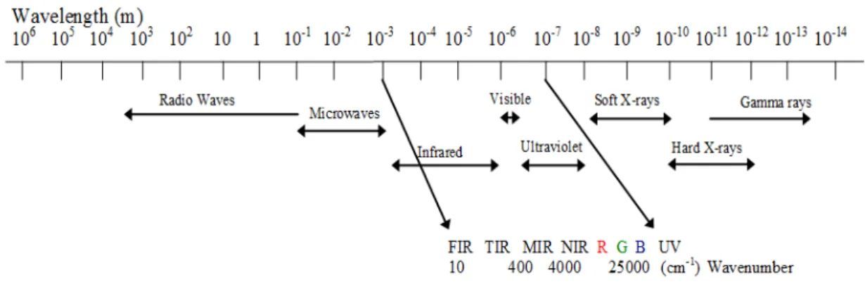
Figure 1. Infrared region of the spectrum consisting of 3 sub regions.. ... 5

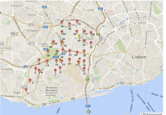
Figure 2. Map of Monsanto Park, Lisbon, in relation to other cities, showing sample collection sites ... 12

Figure 3. Satellite image of Monsanto Park, Lisbon, showing sample collection sites. 13 Figure 4. General topology of the created neural network. ... 19

Figure 5. FTIR spectra of the triplicate samples collected from location 1. ... 21

Figure 6. FTIR spectra of the triplicate samples collected from location 2. ... 22

Figure 7. FTIR spectra of the triplicate samples collected from location 11. ... 22

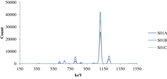
Figure 8. µXRF spectra of the triplicate samples collected from location 1. ... 23

Figure 9. µXRF spectra of the triplicate samples collected from location 2. ... 23

Figure 10. µXRF spectra of the triplicate samples collected from location 11. ... 24

Figure 11. UV spectra for the triplicate samples collected from location 1. ... 25

Figure 12. UV spectra for the triplicate samples collected from location 2. ... 25

Figure 13. UV spectra for the triplicate samples collected from location 11. ... 25

Figure 14. Visible spectra for the triplicate samples collected from location 1. ... 26

Figure 15. Visible spectra for the triplicate samples collected from location 2. ... 26

Figure 16. Visible spectra for the triplicate samples collected from location 11. ... 27

Figure 17. Plot showing the accuracies for the (a) training, (b) testing and (c) validation of the neural network. ... 28

Figure 18. Regression plot of classifier output and expected outcomes for the neural network. ... 29

Figure 19. Error histogram showing the number of instances per interval of error observed. ... 29

List of Tables

Table 1. Sample number and location (GPS co-ordinates). ... 13 Table 2. Dilution factors of the samples for the UV-Visible spectroscopy. ... 16 Table 3. GPS co-ordinates, decimal degrees and Cartesian co-ordinates of the samples.

List of Abbreviations

AAS Atomic Absorption Spectroscopy ANN Artificial Neural Network

ATR Attenuated Total Reflection

EDXRF Energy Dispersive X-ray Fluorescence Spectroscopy ETA Electrothermal Atomisation

FAA Flame Atomic Absorption

FFT-LW Fast Fourier Transform Local Weighted FTIR Fourier Transform Infrared Spectroscopy GPS Global Positioning System

HCl Hydrochloric Acid

ICP Inductively Coupled Plasma

ICP-AES Inductively Coupled Plasma Atomic Emission Spectrometry ICP-MS Inductively Coupled Plasma Mass Spectrometry

ICP-OES Inductively Coupled Plasma Optical Emission Spectrometry IR Infrared Spectroscopy

KOH Potassium Hydroxide

LA-ICP-MS Laser Ablation Inductively Coupled Plasma Mass Spectrometry LDA Linear Discriminant Analysis

LIBS Laser-Induced Breakdown Spectroscopy

MSE Mean Squared Error

NIPALS Nonlinear Iterative Partial Least Squares

NIR Near Infrared

NKj Nitrogen Kjeldahl

PCA Principle Component Analysis PCR Principle Component Regression PLS Partial Least Squares

PLS-LDA Partial Least Squares Linear Discriminant Analysis PSVM Penalised Support Vector Machine

RMSE Route Mean Squared Error RSD Relative Standard Deviation SDA Shrinkage Discriminant Analysis UV-VIS Ultraviolet-Visible Spectroscopy

WDXRF Wavelength Dispersive X-ray Fluorescence Spectroscopy

XRD X-ray Diffraction

1

Introduction

Soil is a complex mixture consisting of crystalline and amorphous minerals, oxides, decomposing organic matter, plants, pollen, microbial residues along with other compounds produced during the formation process (Sugita & Marumo. 1996; Horswell, et al. 2002). Forensic geoscience (analysis of soils and sediment) has been performed for many years for a wide variety of purposes; examples include differentiating between different land use types (Baron et al. 2011), sediment content (Guedes et al. 2009) and the analysis of soil pollutants (Mostert et al. 2010). Due to soils persistence, transferability and Locard’s exchange principle ‘every contact leaves a trace’ (Nickolls, 1956), soil analysis can supply the essential link from the crime scene in question to the suspect and therefore it can be a vital tool. At present, by using a wide range of analytical techniques, crime scene soil samples can be matched to a soil sample taken from a suspect and link them to a particular scene. However, discriminating and characterising soils for intelligence purposes can be much more complex (Baron et al. 2011) due to the enormous variety in composition which is dependent on the location, the type of soil, climate and human activities (Horswell, et al 2002; Pye et al. 2007; Reidy et al. 2013).

Soil composition, type etc. varies from one place to another which can create immense problems when using soil comparisons in legal cases, for the reason that the variation can occur equally within a particular site as much as between sites, and the degree of this is still unknown (Baron et al. 2011). Due to this, it has been documented that is it more straightforward to eliminate soils based on their profiles and compositions than it

is to ‘match’ an unknown sample to a known, taking into account that it is not possible to provide probabilities that another locality may or may not possess the same or very similar characteristics (Morgan & Bull, 2007; Pirrie et al. 2014). One can simply conclude that two samples either do not share a common source or that they are similar in all analytical aspects and therefore cannot be excluded. Forensic soil analysis has already been used in criminal investigations and provided essential information in criminal cases (Dawson et al. 2008; Fitzpatrick & Raven, 2012).

This project aims to develop a method that can be used for intelligence purposes and for that reason this aspect will be the main focus herein. In soil analysis for intelligence purposes, there are two main aspects to be considered in pursuance of excluding samples due to the dissimilarity or including them because they are very similar and these are the physical properties and the chemical properties of the soil samples.

1.1 Physical Properties

1.1.1 Colour Analysis

(2000) used the Munsell Colour Chart to assign Munsell values to soil samples collected from Oregon (USA) before and after pyrolysis. It was found that all the samples had the same pre pyrolysis colour and so pyrolysis was carried out. Even after pyrolysis, some samples still had the same post pyrolysis colour and thus it was determined that another technique must be used in order to differentiate them. Guedes et al. (2009; 2011) demonstrated that measured L*a*b* values were better for discrimination when applied to dried, un-sieved bulk samples as opposed to pre-treated samples, whereas Croft & Pye (2004) suggested removal of organic matter or analysis of each size fractions before and after heat treatment would provide an in-depth analysis.

1.1.2 Granulometry

It has been demonstrated by many authors that granulometry is very useful in soil analysis. Chazottes et al. (2004) found that size distribution of the soil considerably affected results. Particle sizes of 2mm-63µm (unimodal distribution) was found to be

very representative of the ‘original’ soil sample, whereas bimodal distribution (soils

dominated by the extreme particles, those bigger than 4mm and smaller than 20µm, were not very representative. It was suggested than any significant differences in the range of 1mm to 63µm must be considered indicative of dissimilarity between samples. These results are probable due to the fact that bigger particles are more likely to detach from material than smaller particles, leading to a different distribution to control samples.

1.1.3 Palynology

Palynology is pollen and spore science (Hyde & Williams, 1944). Simple palynology consists of pollen and/or spore identification along with pollen and/or spore counting (counting how many times each species occurs within a sample). This allows the creation of a pollen assemblage (profile) which can then help to identify similarities and dissimilarities between samples. It can be a very helpful tool due to the immense variety in the exines (outer shells) making each species unique and the resistive and persistent nature allowing them to survive in particular conditions for thousands of years. It can become complicated if one is not a trained palynologist or someone with little experience due to complexities of pollen identification for example several types of pollen grains can be produced by a single species or grains that look visually similar under a standard microscope come from unrelated plants (Erdtman, 1966).

1.2 Chemical Properties

1.2.1 Infrared (IR) Spectroscopy

Infrared spectroscopy is a well known and used technique in forensic soil analysis as it allows one to analyse the organic and inorganic composition of soils. The IR region of the electromagnetic spectrum ranges from 14000 to 10cm-1 and can be subdivided in to three regions: near, mid and far infrared. Near-infrared ranges from wave numbers from 14000-4000 cm-1_{, mid-infrared ranges from 4000-400 cm}-1 _{and far-infrared ranges from}

400-10 cm-1 _{(Figure 1) (Smith, 1999; Larkin, 2011).}

Fourier transform infrared spectroscopy (FTIR) is a non-destructive technique that requires little sample preparation however the sample must be dried to remove all water as this interferes with the spectrum and samples that are thick allow less infrared light to pass through the sample resulting in a poor signal to noise ratio. IR spectroscopic techniques are extremely sensitive to the organic and inorganic phases of soil (Viscarra Rossel et al. 2006). IR causes vibrations within molecule and these vibrations within particular bonds will only occur at specific wavelengths. This makes it possible to identify functional groups in a molecule and thus the chemical structure and identity of the compound can be confirmed (Haberhauer et al. 1998; Larkin, 2011).

Baron et al. (2011) collected 60 soil samples from 3 different areas in Lincoln, UK. Samples were taken from 4 flower beds, 4 river banks and from 4 woodland sites (each with 5 replicates). Attenuated total reflectance - Fourier transform infrared spectroscopy (ATR-FTIR) was used to collect full spectra from 4000-400 cm-1 using 128 scans with

4cm-1 resolution. The data analysis consisted of nonlinear iterative partial least squares with linear discriminant analysis (NIPALS-LDA) and partial least squares discriminant analysis (PLS-DA). It was found that samples could be completely separated by the land type although it was more difficult to separate the different sites (flower beds, riverbeds and woodland), even after removing regions of the spectra that had poor signal-to-noise ratio. It was concluded that NIPALS-LDA was successful in modelling the 60 spectra into the 3 land-use types although PLS-DA was poor. It was also found that the NIPALS-LDA tool offered a more straightforward and successful approach for modelling but the authors suggest further work is needed as well as more samples, sites and models at different levels to propose a more methodical approach to dataset increases.

Cox et al. (2000) also used FTIR to create spectral profiles of the soil samples by collecting the spectra of the samples, then pyrolysis was carried out and the spectra collected again. The spectrum of the pyrolysed sample was then subtracted from the original so only the organic content spectra remained. There was not sufficient information to repeat this experiment but it was shown to be of use when other techniques cannot distinguish between samples.

accurately. Higher accuracies using local models with small sample sizes was observed whereas Gogé et al. (2014) suggested a decrease in performance with a decrease in sample size (Stafford, 2013).

1.2.2 X-Ray Fluorescence (XRF) Spectroscopy

X-ray fluorescence (XRF) spectroscopy is a multi-elemental technique that can work with different sample forms, is non-destructive, is able to detect elements with atomic numbers greater than 8 and can be used in situ. In an x-ray fluorescence spectrum, the wavelengths present are characteristic of the elements present within the sample. In wavelength dispersive x-ray fluorescence (WDXRF) the samples emitted radiation is diffracted in different directions and a sequential detector moves to detect the x-rays with different wavelengths or a simultaneous detector consisting of fixed single channels to detect specific elements. On the other hand, in energy dispersive XRF (EDXRF) there is only one detector (e.g. (Si(Li))) that is used in combination with a multi-channel analyser according to energies. Although EDXRF is cheaper, WDXRF usually offers greater resolution. Mathematical corrections must be applied to overcome matrix effects that can occur in XRF, which will ensure accurate results are obtained (Levinson, (2001); Krishna et al. (2007); Davidson, 2013).

Yu et al. (2002) used EDXRF to quantify 19 elements in soil samples and determine the source profiles of these samples. Sixteen samples were collected in total, from 2 different sites in 8 different locations. These 8 different locations possessed different geologies; sedimentary, volcanic or granitic. The authors chose EDXRF over ICP-AES or Atomic absorption spectroscopy (AAS) due to its non destructive nature and the ease of analysing solid samples without the need for digestion.

Wavelength Dispersive X-ray Fluorescence Spectroscopy (WDXRF) is not a particularly common technique used in soil analysis. Krishna et al. (2007) used sequential WDXRF to determine the levels of 29 major and trace elements (Si, Al, Fe, Mg, Ca, Na, K, Mn, P, Ti, As, Ba, Cd, Co, Cr, Cu, Se, Sr, Mo, Ni, Pb, Rb, S, U, Th, V, Y, Zn, Zr) in agricultural soil samples. Twenty two international reference materials were used to calibrate the spectrophotometer. The samples were not dried prior to analysis as it was recognised this may cause some loss due to evaporation. Matrix effects caused some difficulties but could be corrected using empirical coefficients (alphas) based on count rate, but when there were high concentrations of some elements in certain samples, this was more difficult to correct. Matrix correction of these samples used carried out using empirical formulas based on concentration but if intensity was used, matrix correction was carried out by trial and error. The relative standard deviation (RSD) for most elements was low at less than 5% but for the elements that had higher RSD; this was most likely due to peak suppression and overlapping peaks. Although matrix correction models can produce accurate results this was not the case when there was a high concentration of heavier elements accompanying the lighter elements. This causes a decrease in accuracy unless the standard used was of similar

composition to that of the ‘unknown’ sample.

Despite the fact that this method had low limits of detection (1-2 mg/kg), good precision and accuracy sufficient for use in agricultural monitoring, it may perhaps have potential for use in a forensic context. However, a lower RSD may be required by reducing the peak suppression. Also, 2g of sample was needed to create the pellets used for this analysis and this is considered a bulk sample in a forensic context and this amount of sample will not always be available and so this method will not be of use in trace analysis.

1.2.3 Inductively Coupled Plasma (ICP) Spectroscopy

is multi elemental are just some clear advantages over other atomic spectroscopy techniques such as flame atomic absorption (FAA), electrothermal atomisation (ETA) or ICP-OES (Thomas, 2013).

Pye & Blott (2009) attempted to create a soil database from 1896 soil samples collected in England and Wales from 1999 to 2007 in connection with casework investigations using ICP-MS and ICP-AES. Two laboratories were used to analyse the samples (one third by only ICP-AES and the rest by both techniques) and the data variation was not significant. Methods used to compare soils on the foundation of elemental composition were developed in the author’s own laboratory. PCA and Euclidean distances were used

to determine the number of elemental concentrations that were indistinguishable for some samples. It was demonstrated that samples that have been taken only a few centimetres apart are likely to be distinguishable based on major and trace elemental concentrations (Stafford, 2013).

After papers demonstrated ICP analysis was a useful technique, Arroyo et al. (2009) validated a laser ablation (LA) ICP-MS method for routine soil and sediment analysis. LA-ICP-MS was found comparable to solution ICP-MS and independent proficiency testing using 57 laboratories found the new method was comparable with conventional digestion ICP and AAS methods. With 3 high speed mills a single technician can prepare around 72 samples per day. This method may have been validated and the values for precision, accuracy are given, but nowhere it is stated which validation guidelines were used (Stafford, 2013).

1.3 Statistical Tools

used PLS along with principle component analysis (PCA) in an attempt to use visible - near infrared (NIR) spectra to create local and national databases and a combination of both to aid in the prediction of soil locations. Guerrero et al. (2010) previously explored something similar to Gogé et al. (2014), where NIR spectral libraries and models were created using PLS regression and then models were spiked with a few samples from target sites (local samples). Croft & Pye (2004) used 4 different techniques to determine the effectiveness of them on different soil types and 5 footwear types and Cox et al. (2000) developed a novel method in which FTIR spectra were collected pre and post pyrolysis which can differentiate samples when other methods cannot.

1.3.1 Artificial Neural Networks

Armenta & de la Guardia (2014) recently reviewed the use of principle component regression (PCR) and PLS, two of the most commonly used techniques for spectral calibration and prediction, and while these are widely used and work well, more sophisticated techniques like artificial neural networks (ANN) have been developed. ANNs are attractive to users because they have incredible information processing characteristics related mainly to nonlinearity, fault and noise tolerance in addition to learning and generalising capabilities (Basheer & Hajmeer, 2000).

Arsoy et al. (2013) used a multilayer feed-forward, with back propagation learning ANN to aid in the prediction of soil water content (SWC) using time domain reflectometry (an electromagnetic method) and found the performance of the ANN was better than that of previous calibration models (using unreliable dielectric permittivity of the soil). 50% of the data was used for training the network and 50% for validation, although no testing was carried out. The ANN had an average route mean squared error (RMSE) of 0.009cm3_cm-3 _{(for 8 nodes) compared to a range of 0.019-0.033 cm}3_cm-3 _for

the calibration model.

of the analyte. Due to the small dataset, the ANN was evaluated by repeating the ANN calculation 5 times, by starting with random weight values to ensure no over fitting occurred. The RMSE was less than 10% when comparing the reference values (from ICP-AES) to the values obtained from the on-site LIBS measurements showing that LIBS is a reliable method.

1.4 Present Work Overview

In this present study, an attempt was made to develop a new method that could reliably and accurately predict the location of known soil samples as well as samples of unknown origin from their FTIR spectra, µXRF profiles and UV-Visible spectra using feature selection and artificial neural networks. In contrast to previous work, the relationship recognised herein is between the input data and the co-ordinates of the samples locations, as opposed to between the input data and soil classes based on the landscape properties.

A systematic attempt was made based on a machine learning approach with feed-forward feature selection and feed-feed-forward neural networks using the values obtained from infrared spectra, µXRF profiles and UV-Visible spectra as input data. A recursive feature selection using a wrapper method was performed using the Boruta (random forest) classifier algorithm. This was performed in order to reduce the input dimensionality and obtain a much smaller subset of features with the highest possible discrimination whilst maintaining excellent neural network performance. This subset of features was used to train, test and validate a neural network.

2

Materials and Methods

2.1 Sample Collection

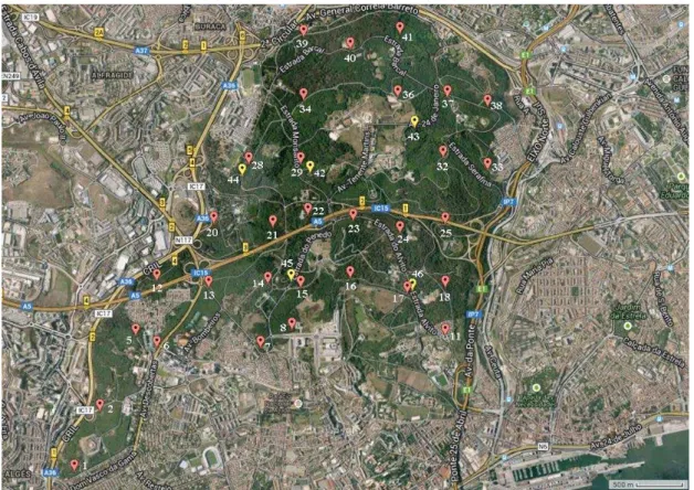
Soil samples were collected from Monsanto Park in Lisbon, Portugal, which has an approximate area of 10km2_{. In total, 31 samples were collected in triplicate (total of 93)}

in 2013 and a further 5 samples were collected in 2014 using a 500 x 500 metre grid of the whole park (Figures 2 and 3). Samples were collected using an in-house built steel core soil sampler with dimensions of 10x3cm, thus samples were collected at a depth of 10cm with a diameter of 3cm and the Global positioning system (GPS) co-ordinates were recorded for each sample site (Table 1) using a Broadcom BCM4750IUB8 GPS receiver.

Figure 3. Satellite image of Monsanto Park, Lisbon, showing sample collection sites (created using batchgeo.com). Red = 2013 Samples, Yellow = 2014 Samples.

Table 1. Sample number and location (GPS co-ordinates).

Sample

Number Latitude Longitude

Sample

2.2 Transfer of GPS Co-ordinates to Cartesian Co-ordinates

The input data for the neural network was FTIR spectral data, XRF spectral data and the palynological data with the output being the sample location. This was achieved by converting the GPS co-ordinates to Cartesian Co-ordinates (x and y co-ordinates). This process is necessary due to the curved nature of the earth’s surface, so if GPS co -ordinates were used this would give non-linear positioning of the samples. Cartesian co-ordinates are easier for the neural network and it also helps to make the interpretation easier on such a small area. Sample 1 is considered to be the starting point of both the x and y axes and the other samples will be relative to this. The GPS co-ordinates were converted from degrees, minutes and seconds in to decimal degrees using the following equation:

Where C is the co-ordinates in decimals, d is the co-ordinates in degrees, m is minutes co-ordinate and s is the seconds co-ordinates. Once converted in to decimal degrees, distances were calculated between samples according to the haversine formula through an in-house built program (table 4).

cos cos

Where d is the distance between 2 points (along the great-circle of a sphere), r is the radius of the sphere, Ø1 and Ø2 are the latitude of sample 1 and 2 respectively and ʎ1

and ʎ2 are the longitude or point 1 and point 2 respectively (Shumaker & Sinnott, 1984)

2.3 FTIR Spectroscopy

2.3.1 Sample Preparation

After collection of all samples, the samples were transported to the laboratory in 50mL Falcon® flasks. These were then transferred in to separate beakers and dried in an oven at 105ºC overnight. Once dried, the samples were sieved through 2mm and 125µm meshes and particles smaller than 125µm were used for the FTIR and UV-Visible analysis.

2.3.2 FTIR Spectroscopy Parameters

The smaller than 125µm portion of the samples were analysed using a PerkinElmer Spectrum 65 spectrophotometer coupled with an attenuated total reflectance (ATR) accessory. The parameters used were a scan range from 4000-400 cm-1, with a resolution of 4 cm-1, 128 scans and with H2O/CO2 correction and the spectra were

collected using % transmission. Baseline corrections were carried out manually using the PerkinElmer Version: 10.03.09.0139 software. In between sample application, the ATR crystal was cleaned with 96% ethanol (Purchased from Carlo Erba Reagents) solution and a background scan was performed after every 3 samples.

2.4 µXRF Spectroscopy 2.4.1 Sample Preparation

Sample preparation was carried out using the following procedure before analysis; into a glass beaker, 3.5g of homogenised sample (using a pestle and mortar) was added and placed into an oven at 80-90ºC overnight to dry the samples and remove any water. A small portion of the dried samples was then transferred on to an acrylic plate, pressed flat and then placed under the laser beam for analysis.

2.4.2 µXRF Spectroscopy Parameters

2.5 UV-Visible Spectroscopy 2.5.1 Sample Preparation

Samples were prepared by adding 0.1g of the 125µm portion of each sample to 1mL of deionised water in 2mL eppendorf tubes, vortexed for 20 seconds and centrifuged for 5mins at 10,000rpm.

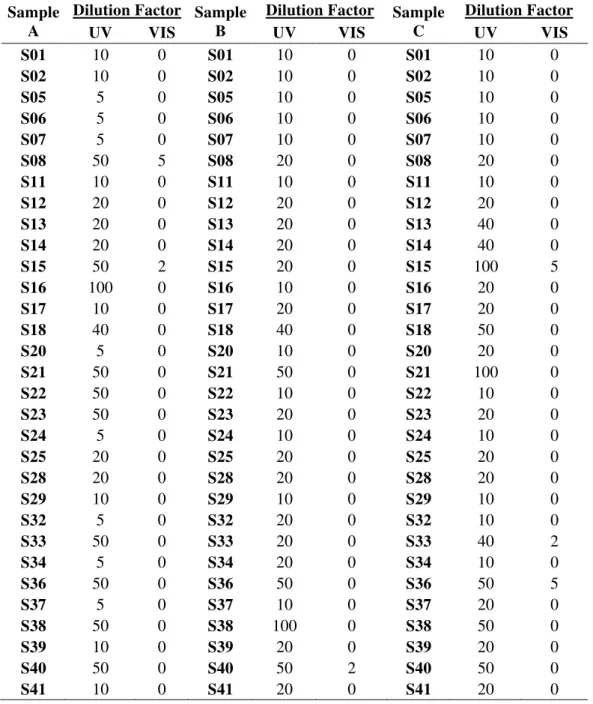
Some samples were too concentrated and so a dilution was carried out with the following factors:

Table 2. Dilution factors of the samples for the UV-Visible spectroscopy.

Sample A

Dilution Factor Sample B

Dilution Factor Sample C

Dilution Factor

UV VIS UV VIS UV VIS

S01 10 0 S01 10 0 S01 10 0

S02 10 0 S02 10 0 S02 10 0

S05 5 0 S05 10 0 S05 10 0

S06 5 0 S06 10 0 S06 10 0

S07 5 0 S07 10 0 S07 10 0

S08 50 5 S08 20 0 S08 20 0

S11 10 0 S11 10 0 S11 10 0

S12 20 0 S12 20 0 S12 20 0

S13 20 0 S13 20 0 S13 40 0

S14 20 0 S14 20 0 S14 40 0

S15 50 2 S15 20 0 S15 100 5

S16 100 0 S16 10 0 S16 20 0

S17 10 0 S17 20 0 S17 20 0

S18 40 0 S18 40 0 S18 50 0

S20 5 0 S20 10 0 S20 20 0

S21 50 0 S21 50 0 S21 100 0

S22 50 0 S22 10 0 S22 10 0

S23 50 0 S23 20 0 S23 20 0

S24 5 0 S24 10 0 S24 10 0

S25 20 0 S25 20 0 S25 20 0

S28 20 0 S28 20 0 S28 20 0

S29 10 0 S29 10 0 S29 10 0

S32 5 0 S32 20 0 S32 10 0

S33 50 0 S33 20 0 S33 40 2

S34 5 0 S34 20 0 S34 10 0

S36 50 0 S36 50 0 S36 50 5

S37 5 0 S37 10 0 S37 20 0

S38 50 0 S38 100 0 S38 50 0

S39 10 0 S39 20 0 S39 20 0

S40 50 0 S40 50 2 S40 50 0

2.5.2 UV-Visible Spectroscopy Parameters

A PerkinElmer Lambda 25 was used to collect ultraviolet (UV) spectra from 400-200cm-1 and visible spectra (VIS) from 1100-401cm-1 using the coloured liquid.After the spectra were collected, the absorbance values were corrected by multiplying the absorbance by the dilution factors used for each sample.

2.6 Palynological Analysis

centrifuged at 3000 rpm for 5 minutes and the liquid decanted. A small quantity of the sample was placed on to a microscope slide, which was covered with a cover glass slip and sealed with a small amount of paraffin. Samples were then analysed using an Olympus CX21 biological microscope at 1000X magnification and the pollen grains were identified and counted to a maximum of 100 per slide.

The deionised water was produced in-house with a resistance of 15MΩ using a Helix 10 Millipore and potassium hydroxide was made using KOH pellets purchased from EKA Chemicals with deionised water.

2.7 Input Vectors

Pre-processing of feature vectors were carried out prior to the training of the neural network. All IR spectra were manually baseline corrected, so the baseline was a maximum of 100% transmittance. The UV-Visible spectra were normalised correcting for the dilution factors. Discriminatory peaks present in all the spectra for UV, visible, FTIR and XRF were then manually selected. 20 features were manually selected for visible, 6 for UV and 27 features for both FTIR and µXRF. The relationship between each of these features was then computed for each method separately.

2.8 Feature Selection

Feature selection was performed on 1430 manually selected features with the purpose of reducing the dimensionality of the input vectors, with the aim of ascertaining a subset of features, with the smallest size which provided the highest possible discrimination between samples. A recursive feature selection wrapper method (Boruta) based on random forest was used in R version 2.15.2 (R Development Core Team, 2008). Input vectors were computed by the feature selection method used and consequently used for the training and selection of one neural network.

2.9 Artificial Neural Network

MATLABs’ (The MathWorks, 2011a) Neural Networks Toolbox (The MathWorks,

2011b) was used to develop feed forward fully connected neural networks. The neural networks weights and biases were initialised using the Nguyen-Widrow layer initialisation function, which initialises weights and biases randomly although evenly

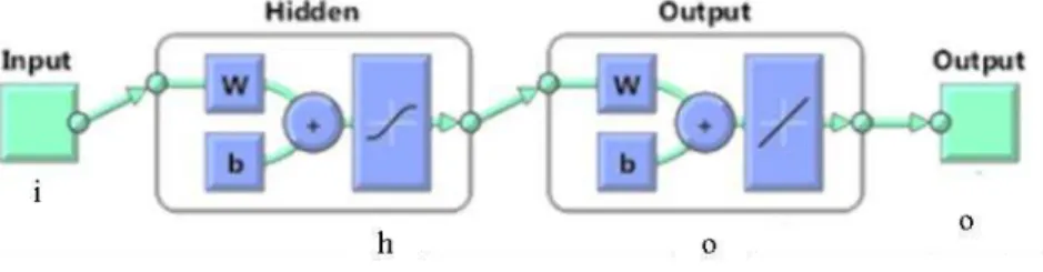
activation function for the hidden layer and the linear function was chosen for the output layer. The scaled conjugate gradient back propagation (backward propagation of errors) was used as the learning algorithm and the mean absolute error was the performance measure used to stop training. The number of neuron present in the hidden layer was computed based on the number of dimensions of the feature vectors and the number of neurons in the output layer was two, corresponding to x,y co-ordinates of the samples. A general topology of a neural network is shown in figure 4.

Figure 4. General topology of the created neural network, where i relates to the number of the inputs present in the input vector, w relates to the weights, b relates to the bias, h is the number of neurons in the hidden layer and o is the output vector number.

3

Results and Discussion

3.1 Sample Collection

Some of the planned sites for sampling were not possible to reach due to the land being privately owned and thus no permission to collect and so samples were collected at the nearest achievable location.

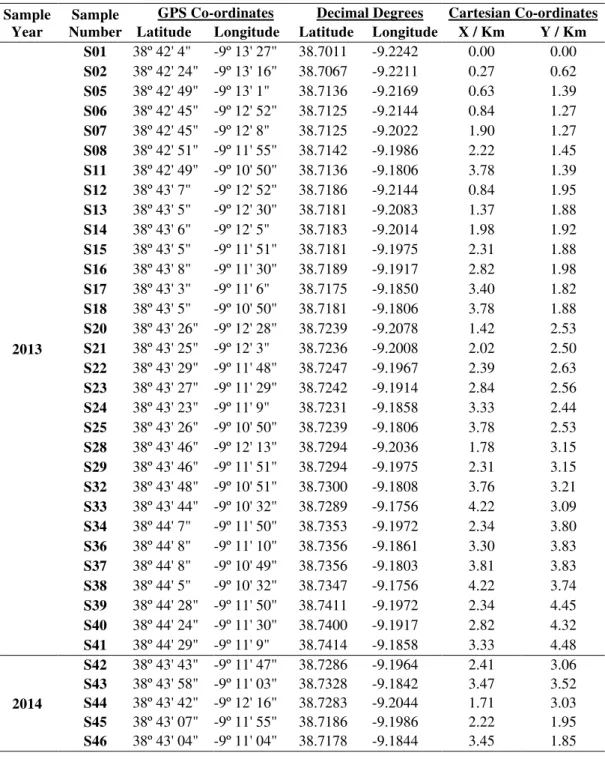
Table 3. GPS co-ordinates, decimal degrees and Cartesian co-ordinates of the samples.

Sample

Year Number Sample

GPS Co-ordinates Decimal Degrees Cartesian Co-ordinates

Latitude Longitude Latitude Longitude X / Km Y / Km

2013

S01 38º 42' 4" -9º 13' 27" 38.7011 -9.2242 0.00 0.00 S02 38º 42' 24" -9º 13' 16" 38.7067 -9.2211 0.27 0.62 S05 38º 42' 49" -9º 13' 1" 38.7136 -9.2169 0.63 1.39 S06 38º 42' 45" -9º 12' 52" 38.7125 -9.2144 0.84 1.27 S07 38º 42' 45" -9º 12' 8" 38.7125 -9.2022 1.90 1.27 S08 38º 42' 51" -9º 11' 55" 38.7142 -9.1986 2.22 1.45 S11 38º 42' 49" -9º 10' 50" 38.7136 -9.1806 3.78 1.39 S12 38º 43' 7" -9º 12' 52" 38.7186 -9.2144 0.84 1.95 S13 38º 43' 5" -9º 12' 30" 38.7181 -9.2083 1.37 1.88 S14 38º 43' 6" -9º 12' 5" 38.7183 -9.2014 1.98 1.92 S15 38º 43' 5" -9º 11' 51" 38.7181 -9.1975 2.31 1.88 S16 38º 43' 8" -9º 11' 30" 38.7189 -9.1917 2.82 1.98 S17 38º 43' 3" -9º 11' 6" 38.7175 -9.1850 3.40 1.82 S18 38º 43' 5" -9º 10' 50" 38.7181 -9.1806 3.78 1.88 S20 38º 43' 26" -9º 12' 28" 38.7239 -9.2078 1.42 2.53 S21 38º 43' 25" -9º 12' 3" 38.7236 -9.2008 2.02 2.50 S22 38º 43' 29" -9º 11' 48" 38.7247 -9.1967 2.39 2.63 S23 38º 43' 27" -9º 11' 29" 38.7242 -9.1914 2.84 2.56 S24 38º 43' 23" -9º 11' 9" 38.7231 -9.1858 3.33 2.44 S25 38º 43' 26" -9º 10' 50" 38.7239 -9.1806 3.78 2.53 S28 38º 43' 46" -9º 12' 13" 38.7294 -9.2036 1.78 3.15 S29 38º 43' 46" -9º 11' 51" 38.7294 -9.1975 2.31 3.15 S32 38º 43' 48" -9º 10' 51" 38.7300 -9.1808 3.76 3.21 S33 38º 43' 44" -9º 10' 32" 38.7289 -9.1756 4.22 3.09 S34 38º 44' 7" -9º 11' 50" 38.7353 -9.1972 2.34 3.80 S36 38º 44' 8" -9º 11' 10" 38.7356 -9.1861 3.30 3.83 S37 38º 44' 8" -9º 10' 49" 38.7356 -9.1803 3.81 3.83 S38 38º 44' 5" -9º 10' 32" 38.7347 -9.1756 4.22 3.74 S39 38º 44' 28" -9º 11' 50" 38.7411 -9.1972 2.34 4.45 S40 38º 44' 24" -9º 11' 30" 38.7400 -9.1917 2.82 4.32 S41 38º 44' 29" -9º 11' 9" 38.7414 -9.1858 3.33 4.48

2014

3.2 FTIR Spectra

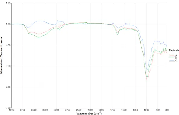
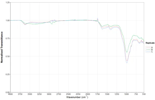
Figures 5 and 6 show the FTIR spectra of the triplicates collected for samples 1 and 2. The spectral profiles both samples are quite similar, including the transmittance of the peaks and this is the same across most of the samples, so to the naked eye it is difficult to differentiate between some samples. Figure 7 shows sample 11 has a very different profile across most of the spectrum with a peak at 2500cm-1 _{that is not present in figures}

5 or 6. This was not surprising as the colour of sample 11 was light beige whereas samples 1 and 2 were dark brown and thus the organic composition differs greatly between the samples. The spectrum from 549-400cm-1 has been removed from all spectra due to the increased noise and low resolution present in this region. All other sample spectra are present on the appendix disk.

Figure 6. FTIR spectra of the triplicate samples collected from location 2.

3.3 µXRF Profiles

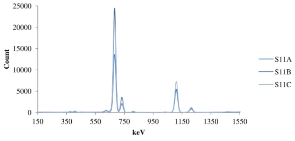
Like with the FTIR spectra the XRF profiles sample 1 and 2 (figures 8 and 9) are very similar although the counts for the different elements differ between samples and the ratios between the different peaks differ also. Figure 10 (Sample 11) has a very different profile to samples 1 and 2 which was not unexpected as the FTIR spectra were very different. All other sample spectra are present on the appendix disk.

Figure 8. µXRF spectra of the triplicate samples collected from location 1.

Figure 9. µXRF spectra of the triplicate samples collected from location 2. 0

10000 20000 30000 40000 50000

150 350 550 750 950 1150 1350 1550

Co

unt

keV

S01A S01B S01C

0 10000 20000 30000 40000 50000

150 350 550 750 950 1150 1350 1550

Co

unt

keV

Figure 10. µXRF spectra of the triplicate samples collected from location 11.

3.4 UV-Visible Spectra

3.4.1 UV-Spectra

Figures 11 and 12 show the corrected UV spectra of samples 1 and 2 have very different profiles across the spectrum but there are some similarities. There are clear differences in the absorbances of each spectrum, within the triplicate samples as well as between the samples. The peak at 260nm and the trough at 220nm is present in almost all samples although the profile to the left and right of the peak and the absorbances differ between samples. Figure 13 shows sample 11B and C have similar profiles to that of samples 1C and 2C. Sample 11A has a very different profile to that of 11B and C as well as samples 1 and 2. All other sample spectra are present on the appendix disk.

0 5000 10000 15000 20000 25000

150 350 550 750 950 1150 1350 1550

Co

unt

keV

Figure 11. UV spectra for the triplicate samples collected from location 1.

Figure 12. UV spectra for the triplicate samples collected from location 2.

Figure 13. UV spectra for the triplicate samples collected from location 11. 0 2 4 6 8 10

200 250 300 350 400

Ab

so

rban

ce

Wavelength / nm

S01A S01B S01C 0 2 4 6 8 10 12 14

200 250 300 350 400

Ab

so

rban

ce

Wavelength / nm

S02A S02B S02C 0 2 4 6 8 10

200 250 300 350 400

Ab

so

rban

ce

Wavelength / nm

3.4.2 Visible Spectra

Figures 14 and 15 show the normalised visible spectra of samples 1 and 2 have similar profiles across the spectrum but there are distinct differences in the absorbance values, where sample 2 has absorbances almost twice that of sample 2. This is the case when looking at the spectra of all the other samples, with very little specific peaks or discrete features present in the visible region. Figure 16 shows sample 11 which has a similar profile to samples 1 and 2 although the B samples have higher absorbance’s than the A and C samples. All other sample spectra are present on the appendix disk.

Figure 14. Visible spectra for the triplicate samples collected from location 1.

Figure 15. Visible spectra for the triplicate samples collected from location 2. 0

0.1 0.2 0.3 0.4

400 500 600 700 800 900 1000 1100

No rmali sed Ab so rban ce Wavelength (nm) S01A S01B S01C 0 0.2 0.4 0.6 0.8

400 500 600 700 800 900 1000 1100

Figure 16. Visible spectra for the triplicate samples collected from location 11.

The actual profile and values of the peaks present in the samples is not of crucial importance as the neural network uses the relationship between the peaks present in the spectra.

3.5 Palynological Analysis

Due to the samples over processing, no surface features were left on the pollen, making it impossible to identify them and thus unfortunately it was not possible to complete the palynological analysis due to the method failing to work as expected.

3.6 Selected Features

Peaks were manually selected from the different spectra. From the visible spectra 5 features, from UV 3 features, from FTIR 27 features and XRF 27 features were identified. The relationship between each feature was computed by dividing each feature by the others. For example, if there are 3 features, A, B and C. The total number of features was calculated by A/B, A/C, B/A, B/C, C/A and C/B, so now there is a total of 6 features selected. This was carried out for each different technique separately. In total, 1430 features were selected for the 4 different methods which were then submitted to Boruta.

0 0.2 0.4 0.6 0.8

400 500 600 700 800 900 1000 1100

No

rmali

sed

Ab

so

rban

ce

Wavelength (nm)

3.7 Feature Selection

The Boruta algorithm was used, which selected a total of 43 features from the 1430 total (table 4 in appendix) and these features were then used in the training of the neural network. There were 25 features selected from the FTIR, 15 from µXRF, and 3 from the visible spectra, however, no features were selected from the UV spectra.

3.8 Neural Network

Initially, 1000 neural networks were created and the best one was chosen. Figure 17 shows the training (figure 17a) had the greatest accuracy of 90%, the accuracy of the testing (figure 17b) had a much lower accuracy of 74% and validation (figure 17c) had an accuracy of 79%. Figure 18 shows that the overall linear correlation factor (accuracy) obtained was 86%. The error histogram that was obtained (figure 19) shows the errors are mainly occurring around zero for the input vectors. Figure 20 shows the MSE for training, testing and validation and the plot shows that the neural network is not to over fitted and the MSE’s are very low.

Figure 18. Regression plot of classifier output and expected outcomes for the neural network.

Figure 19. Error histogram showing the number of instances per interval of error observed (blue bars for training, red bars for testing and green bars for validation).

4

Conclusion

The neural network was able to produce a correlation factor of 86% using the Boruta (random trees) algorithm, using FTIR, µXRF and visible spectroscopy data. No features were selected from the UV spectra showing that UV is not a useful technique to use in this method. Only 3 features were manually identified in this region, but these were not discriminatory enough to be used to differentiate the different samples, thus they were not selected during the feature selection process. It was also not possible to collect and therefore use any palynological data, due to the samples being over processed since method failed to work as expected.

The accuracy achieved with this study (86%) is a marked improvement on 77% using just FTIR spectra, so it can be concluded that by adding µXRF and visible spectroscopy data the accuracy of the prediction is greatly increased. The improved accuracy of this method demonstrates how powerful multiple techniques can be in soil analysis and that this is a strong method that could be widely used.

5

Recommendations for Further Work

Prospects for the future could be to increase the amount of data input into the neural network by using more techniques which should increase the accuracy of the prediction.

Increase the number of samples by expanding the grid used and reducing the distance between collection sites which will increase the usefulness of this technique.

The samples could be re-analysed on a FTIR with a cleaner or new crystal to reduce noise in the spectra.

Analyse the 2014 samples using FTIR, µXRF and visible spectroscopy to determine if the method is reproducible across different years.

Also, test different feature selection methods, to see if this increases the number of selected features and improves the overall accuracy of the neural network.

References

Arsoy, S., Ozgur, M., Keskin, E., & Yilmaz, C. (2013). Enhancing TDR based water content measurements by ANN in sandy soils. Geoderma, 195-196, 133–144. doi:10.1016/j.geoderma.2012.11.019

Baron, M., Gonzalez-Rodriguez, J., Croxton, R., Gonzales, R., & Jimenez-Perez, R. (2011). Chemometric Study on the Forensic Discrimination of Soil Types Using Their Infrared Spectral Characteristics. Applied Spectroscopy, 65(10), 1151–1161. doi:10.1366/10-06197

Basheer, I. A., & Hajmeer, M. (2000). Artificial neural networks: fundamentals, computing, design, and application. Journal of Microbiological Methods, 43(1), 3–

31. doi: 10.1016/S0167-7012(00)00201-3

Carvalho, Á., Ribeiro, H., Mayes, R., Guedes, A., Abreu, I., Noronha, F., & Dawson, L. (2013). Organic matter characterization of sediments in two river beaches from northern Portugal for forensic application. Forensic Science International, 233(1-3), 403–415. doi:10.1016/j.forsciint.2013.10.019

Chazottes, V., Brocard, C., & Peyrot, B. (2004). Particle size analysis of soils under simulated scene of crime conditions: the interest of multivariate analyses. Forensic Science International, 140(2-3), 159–166. doi:10.1016/j.forsciint.2003.11.032

Cox, R. J., Peterson, H. L., Young, J., Cusik, C., & Espinoza, E. O. (2000). The forensic analysis of soil organic by FTIR. Forensic Science International, 108(2), 107–116. doi:10.1016/S0379-0738(99)00203-0

Croft, D. J., & Pye, K. (2004). Multi-technique comparison of source and primary transfer soil samples: an experimental investigation. Science & Justice : Journal of the Forensic Science Society, 44(1), 21–28. doi:10.1016/S1355-0306(04)71681-0

Dawson, L. A., Campbell, C. D., Hillier, S., & Brewer, M. J. (2008). Methods of Characterizing and Fingerprinting Soils for Forensic Application. In M. Tibbett & D. Carter (Eds.), Soil Analysis In Forensic Taphonomy (pp. 271–315). Boca Raton,: CRC Press. doi:10.1201/9781420069921

De Vos, W., & Viaene, W. (1980) Geochemical study of solid and metallogenetic implications at Hiendelaencina, Guadalajara, Spain. Mineralium Deposita 15(1) 87-99. doi: 10.1007/BF00202848

Du, C., Ma, Z., Zhou, J., & Goyne, K. W. (2013). Application of mid-infrared photoacoustic spectroscopy in monitoring carbonate content in soils. Sensors and Actuators B: Chemical, 188, 1167–1175. doi:10.1016/j.snb.2013.08.023

El Haddad, J., Bruyère, D., Ismaël, A., Gallou, G., Laperche, V., Michel, K., Canioni, L., & Bousquet, B. (2014). Application of a series of artificial neural networks to on-site quantitative analysis of lead into real soil samples by laser induced breakdown spectroscopy. Spectrochimica Acta Part B: Atomic Spectroscopy, 97, 57–64. doi:10.1016/j.sab.2014.04.014

Erdtman, G. (1966) Pollen morphology and plant taxonomy: Angiosperms. New York, USA: Hafner Publishing Company.

Fitzpatrick, R. W. (2009). Soil: Forensic analysis. In A. Jamieson & A. Moenssens (Eds.), Wiley Encyclopedia Of Forensic Science (pp. 2377 – 2388). Chichester, UK: John Wiley & Sons, Ltd. doi:10.1002/9780470061589

Ge, Y., Morgan, C. L. S., Grunwald, S., Brown, D. J., & Sarkhot, D. V. (2011). Comparison of soil reflectance spectra and calibration models obtained using multiple spectrometers. Geoderma, 161(3-4), 202–211. doi:10.1016/j.geoderma.2010.12.020

Guedes, A., Ribeiro, H., Valentim, B., & Noronha, F. (2009). Quantitative colour analysis of beach and dune sediments for forensic applications: a Portuguese example. Forensic Science International, 190(1-3), 42–51. doi:10.1016/j.forsciint.2009.05.010

Guedes, A., Ribeiro, H., Valentim, B., Rodrigues, A., Sant’Ovaia, H., Abreu, I., &

Noronha, F. (2011). Characterization of soils from the Algarve region (Portugal): a multidisciplinary approach for forensic applications. Science & Justice : Journal of the Forensic Science Society, 51(2), 77–82. doi:10.1016/j.scijus.2010.10.006

Guerrero, C., Zornoza, R., Gómez, I., & Mataix-Beneyto, J. (2010). Spiking of NIR regional models using samples from target sites: Effect of model size on prediction accuracy. Geoderma, 158(1-2), 66–77. doi:10.1016/j.geoderma.2009.12.021

Haberhauer, G., Rafferty, B., Strebl, F., & Gerzabek, M. H. (1998). Comparison of the composition of forest soil litter derived from three different sites at various decompositional stages using FTIR spectroscopy. Geoderma, 83(3-4), 331–342. doi:10.1016/S0016-7061(98)00008-1

Horswell, J., Cordiner, S. J., Maas, E. W., Martin, T. M., Sutherland, K. B. W., Speir, T. W., Nogales, B., & Osborn, A M. (2002). Forensic comparison of soils by bacterial community DNA profiling. Journal of Forensic Sciences, 47(2), 350–353. Retrieved from http://www.ncbi.nlm.nih.gov/pubmed/11911110

Hyde, H.A. & Williams, D.A. (1994) The right word. Pollen Science Circular. No.8 p. 6

Krishna, A.K., Murthy, N.N., & Govil, P.K. (2007) Multielement Analysis of Soils by Wavelength-Dispersive X-ray Fluorescence Spectrometry. Atomic Spectroscopy, 28(6) 202-214. doi:10.1007/BF02991248

Kuhn, M. (2008). Building predictive models in R using the caret package. Journal Of Statistical Software, 28(5), 1–26. Retrieved from http://www.jstatsoft.org/v28/i05/

Levinson, R. (2001) More modern chemical techniques. London, UK: Royal Society of Chemistry

Mildenhall, D. C. (1990). Forensic palynology in New Zealand. Review of

Palaeobotany and Palynology, 64(1-4), 227–234.

doi:10.1016/0034-6667(90)90137-8

Mildenhall, D. C. (2006). An unusual appearance of a common pollen type indicates the scene of the crime. Forensic Science International, 163(3), 236–240. doi:10.1016/j.forsciint.2005.11.029

Morgan, R. M., & Bull, P. A. (2007). The use of grain size distribution analysis of sediments and soils in forensic enquiry. Science & Justice : Journal of the Forensic Science Society, 47(3), 125–135. doi:10.1016/j.scijus.2007.02.001

Morgan, R. M., Flynn, J., Sena, V., & Bull, P. A. (2014). Experimental forensic studies of the preservation of pollen in vehicle fires. Science & Justice : Journal of the Forensic Science Society, 54(2), 141–145. doi:10.1016/j.scijus.2013.04.001

Mostert, M. M. R., Ayoko, G. A., & Kokot, S. (2010). Application of chemometrics to analysis of soil pollutants. TrAC Trends in Analytical Chemistry, 29(5), 430–445. doi:10.1016/j.trac.2010.02.009

Mularczyk-Oliwa, M., Bombalska, A., Kaliszewski, M., Włodarski, M., Kopczyński, K., Kwaśny, M., Szpakowska, M., & Trafny, E. A. (2012). Comparison of

fluorescence spectroscopy and FTIR in differentiation of plant pollens. Spectrochimica Acta. Part A, Molecular and Biomolecular Spectroscopy, 97, 246– 254. doi:10.1016/j.saa.2012.05.063

Nickolls, L. C. (1956). The scientific investigation of crime. (Lewis C. Nickolls, Ed.) (p. 398). London: Butterworth

Pye, K., & Blott, S. J. (2004). Particle size analysis of sediments, soils and related particulate materials for forensic purposes using laser granulometry. Forensic Science International, 144(1), 19–27. doi:10.1016/j.forsciint.2004.02.028

Pye, K., & Blott, S. J. (2009). Development of a searchable major and trace element database for use in forensic soil comparisons. Science & Justice : Journal of the Forensic Science Society, 49(3), 170–181. doi:10.1016/j.scijus.2009.02.007

Pye, K., Blott, S. J., Croft, D. J., & Witton, S. J. (2007). Discrimination between sediment and soil samples for forensic purposes using elemental data: an investigation of particle size effects. Forensic Science International, 167(1), 30–

42. doi:10.1016/j.forsciint.2006.06.005

Pye, K., & Croft, D. J. (2004). Forensic geoscience: introduction and overview.

Geological Society, London, Special Publications, 232(1), 1–5.

doi:10.1144/GSL.SP.2004.232.01.01

R Development Core Team. (2008). R: A language and environment for statistical computing (Version 2.15.2). Vienna, Austria: R Foundation for Statistical Computing.

Reidy, L., Bu, K., Godfrey, M., & Cizdziel, J. V. (2013). Elemental fingerprinting of soils using ICP-MS and multivariate statistics: A study for and by forensic chemistry majors. Forensic Science International, 233(1-3), 37–44. doi:10.1016/j.forsciint.2013.08.019

Shumaker, B. P. & Sinnott, R. W. (1984). Virtues of the haversine. Sky Telesc., 68(2), 158–159

Singh, V., & Agrawal, H. M. (2012). Qualitative soil mineral analysis by EDXRF, XRD and AAS probes. Radiation Physics and Chemistry, 81(12), 1796–1803. doi:10.1016/j.radphyschem.2012.07.002

Stafford, H. L. (2013) Statistics Assignment: Critical review of published articles related to soil and sediment analyses with statistical analyses. M. Sc. Assignment. University of Lincoln

Sugita, R., & Marumo, Y. (1996). Validity of color examination for forensic soil identification. Forensic Science International, 83(3), 201–210. doi:10.1016/S0379-0738(96)02038-5

The MathWorks, I. (2011a). MATLAB. Massachusetts, United States: The MathWorks, Inc.

The MathWorks, I. (2011b). Neural networks toolbox for MATLAB. Massachusetts, United States: The MathWorks, Inc.

Thomas, R., (2013) Practical guide to ICP-MS - A tutorial for beginners (3rd Ed.). Florida, USA: CRC Press

Viscarra Rossel, R. A., Walvoort, D. J. J., McBratney, A. B., Janik, L. J., & Skjemstad, J. O. (2006). Visible, near infrared, mid infrared or combined diffuse reflectance spectroscopy for simultaneous assessment of various soil properties. Geoderma, 131(1-2), 59–75. doi:10.1016/j.geoderma.2005.03.007

Appendix

Table 4. Features selected by the Boruta feature selection algorithm, showing the relationship between peaks.

Feature Number V1 V2 Feature Number V1 V2

6 VIS_980 VIS_905 590 FTIR_700 FTIR_755

10 VIS_905 VIS_980 592 FTIR_700 FTIR_725

15 VIS_800 VIS_905 619 FTIR_671 FTIR_710

54 FTIR_1747 FTIR_1630 683 FTIR_569 FTIR_990

80 FTIR_1630 FTIR_1747 709 FTIR_555 FTIR_990

190 FTIR_990 FTIR_910 723 FTIR_555 FTIR_710

192 FTIR_990 FTIR_870 866 XFR_3.292 XFR_4.4983 216 FTIR_925 FTIR_910 867 XFR_3.292 XFR_4.9193 242 FTIR_910 FTIR_925 942 XFR_4.4983 XFR_3.292 293 FTIR_870 FTIR_990 948 XFR_4.4983 XFR_6.4837 294 FTIR_870 FTIR_925 953 XFR_4.4983 XFR_7.9351 319 FTIR_850 FTIR_990 955 XFR_4.4983 XFR_8.6514 351 FTIR_810 FTIR_800 958 XFR_4.4983 XFR_14.0296 352 FTIR_810 FTIR_785 968 XFR_4.9193 XFR_3.292 377 FTIR_800 FTIR_810 1118 XFR_7.3508 XFR_18.3397 403 FTIR_785 FTIR_810 1140 XFR_7.5832 XFR_14.0296 409 FTIR_785 FTIR_725 1179 XFR_7.9351 XFR_4.4983 435 FTIR_775 FTIR_725 1192 XFR_7.9351 XFR_14.0296 486 FTIR_755 FTIR_737 1231 XFR_8.6514 XFR_4.4983 538 FTIR_725 FTIR_755 1309 XFR_14.0296 XFR_4.4983 541 FTIR_725 FTIR_700 1335 XFR_15.7197 XFR_4.4983 568 FTIR_710 FTIR_671

See Appendix Disk for:

FTIR Spectra UV Spectra Visible Spectra XRF Spectra