www.ocean-sci.net/12/379/2016/ doi:10.5194/os-12-379-2016
© Author(s) 2016. CC Attribution 3.0 License.
Remote sensing of chlorophyll in the Baltic Sea at basin scale
from 1997 to 2012 using merged multi-sensor data
Jaime Pitarch1, Gianluca Volpe1, Simone Colella1, Hajo Krasemann2, and Rosalia Santoleri1 1Institute for Climate and Atmospheric Sciences, Italian National Research Council, Via del Fosso del Cavaliere 100, 00133 Rome, Italy
2Helmholtz-Zentrum Geesthacht, Centre for Materials and Coastal Research GmbH, Max-Planck-Strasse 1, 21502 Geesthacht, Germany
Correspondence to: Jaime Pitarch ([email protected])
Received: 9 September 2015 – Published in Ocean Sci. Discuss.: 30 September 2015 Revised: 1 February 2016 – Accepted: 23 February 2016 – Published: 8 March 2016
Abstract. A 15-year (1997–2012) time series of chloro-phyll a (Chla) in the Baltic Sea, based on merged multi-sensor satellite data was analysed. Several available Chl a algorithms were sea-truthed against the largest in situ pub-licly available Chl a data set ever used for calibration and validation over the Baltic region. To account for the known biogeochemical heterogeneity of the Baltic, matchups were calculated for three separate areas: (1)the Skagerrak and Kat-tegat, (2) the central Baltic, including the Baltic Proper and the gulfs of Riga and Finland, and (3) the Gulf of Both-nia. Similarly, within the operational context of the Coperni-cus Marine Environment Monitoring Service (CMEMS) the three areas were also considered as a whole in the analy-sis. In general, statistics showed low linearity. However, a bootstrapping-like assessment did provide the means for re-moving the bias from the satellite observations, which were then used to compute basin average time series. Resulting climatologies confirmed that the three regions display com-pletely different Chlaseasonal dynamics. The Gulf of Both-nia displays a single Chl a peak during spring, whereas in the Skagerrak and Kattegat the dynamics are less regular and composed of highs and lows during winter, progressing to-wards a small bloom in spring and a minimum in summer. In the central Baltic, Chlafollows a dynamics of a mild spring bloom followed by a much stronger bloom in summer. Sur-face temperature data are able to explain a variable fraction of the intensity of the summer bloom in the central Baltic.
1 Introduction
dis-solved organic matter (CDOM) and non-algal particles. Both types of algorithms are very sensitive to the in situ observa-tions used to calibrate them, thus providing the motivation of the regionalization approach adopted within CMEMS. Those based on neural network constitute a third kind of algorithms for Chla retrieval whose limitations are, in theory, the same as the first two: strong dependency on the training data sets that limit their overall applicability. Here, all three kinds of algorithms are tested.
The Baltic Sea is a semi-enclosed basin bordering the North Sea in correspondence of the Danish archipelago. The Skagerrak and Kattegat are generally not associated with the Baltic Sea. However, the Baltic domain that is defined within CMEMS extends the eastern limit to the meridian 9.24◦E, thus including most of the Skagerrak basin and the
entire Kattegat basin. The Baltic is characterized by signif-icant CDOM concentration due to high river runoff. It is known that high CDOM concentration reduces the water-leaving radiance, making the seawater darker (Berthon and Zibordi, 2010), which constitutes one of the main challenges for ocean colour algorithms to work properly over the Baltic Sea (Mélin and Vantrepotte, 2015). Despite the fact that the Baltic Sea is widely recognized as a challenging test bed for remote sensing, literature on calibration and validation of Chl a algorithms is not abundant. Standard algorithms are those provided by the space agencies for global and op-erational applications. The application of these algorithms to the in situ remote-sensing reflectance (Rrs), collected in 707 stations off Poland between 1993 and 2001, revealed un-certainties exceeding 100 % when the output was compared against collocated Chlameasurements (Darecki and Stram-ski, 2004). Even less encouraging results were obtained when four standard Chlaalgorithms were applied to Sea-viewing Wide Field-of-view Sensor (SeaWiFS) images between 2000 and 2001 (HELCOM, 2004). Matchup with 75 Chl a pro-files across all the Baltic Sea, with predominance of Swedish coastal waters, gave virtually null correlation, with satellite Chl a underestimating the in situ Chla by 180 to 500 %, in contradiction with Darecki and Stramski (2004). More re-cently, the Case II Regional, Boreal, and Eutrophic MERIS processors were applied to images between 2006 and 2009 (Attila et al., 2013). Matchup with 312 stations in the Gulf of Finland and in the central Baltic Sea showed large Chla overestimation. However, when the standard bio-optical rela-tionships of these processors were tuned with the local in situ Chla, the bias did reduce significantly (Fig. 6 in Attila et al., 2013). The heterogeneity of results combined with the lim-ited spatial and temporal representativeness of the in situ ob-servations used in the mentioned data comparisons prompts further investigation. This work aims to fill this gap by using the largest, publicly available in situ data set ever used over the Baltic Sea for validation activities.
There is extensive literature on the biogeochemistry of the Baltic Sea and its relation to physics. River outflows release large amounts of organic matter, which sinks to the
bot-tom and lowers the oxygen concentration, leading to large amounts of phosphate to be released by the sediment and upwelled through complex mixing processes (Reissmann et al., 2009). In spring, a nutrient-enriched hypolimnion and warmer temperatures trigger diatom and dinoflagel-late blooms, depleting nitrogen. In summer, nitrogen-fixing cyanobacteria take advantage of the relatively phosphate-rich, calm and warm surface waters, producing another bloom (Reissmann et al., 2009). The central Baltic Sea is characterized by summer blooms of cyanobacteria that are known to have a buoyancy regulation ability (e.g. N. spumi-gena and Aphanizomenon sp., Ibelings et al., 1991) and that, under calm conditions, can accumulate at the sea sur-face (Ploug, 2008). Cyanobacteria blooms are commonly ob-served in the central Baltic Proper but not in the Skagerrak and Kattegat nor in the Gulf of Bothnia (Wasmund and Uh-lig, 2003). The Skagerrak and Kattegat are subject to much higher influence from the North Sea, so that the phytoplank-ton dynamics here are expected to be different than those at the Baltic Sea. Thus, there is a strong need for the calibration and validation of the proposed algorithms to take account of the complex morphology and biogeochemistry of the basin. Algorithms are then tested in four geographical areas: (1) the Skagerrak and Kattegat, (2) the Baltic Proper and the gulfs of Riga and Finland, here referred to as “Central Baltic”, (3) the Gulf of Bothnia, and (4) the entire area (1–3).
Ocean colour has cloud cover as an additional problem, which is particularly high over northern Europe. To increase the spatial coverage of daily products, the International Ocean-Colour Coordinating Group (IOCCG) recommended the merging of ocean colour data from multiple missions (IOCCG, 2007). At the European level, the Climate Change Initiative (CCI) program (www.esa-oceancolour-cci.org) and the Globcolour (www.globcolour.info) project followed this recommendation and reprocessed archived data from vari-ous medium-resolution sensors. Here, the CCI-derived Rrs are used as input to the Chla algorithms for the compari-son exercise (see Sect. 2.1 for their description). One of the limitations of this approach is given by the fact that the CCI does not include any near-infrared bands, which are known to be better suited than the blue–green bands for Case II wa-ters (Odermatt et al., 2012). On the other hand, merged data span for longer time periods (1997–2012) than any of the in-dividual sensors alone and provide higher coverage on a daily basis.
dy-namics data over the entire Baltic region are still lacking, de-spite the fact that these are required by the European Water Framework Directive for coastal and inland waters and by the Marine Strategy Framework Directive for open ocean waters. In this article, we aim to partially fill this gap by focusing on long-term remote sensing of Chlaat the basin scale.
2 Data and methods 2.1 Satellite Chladata
The GlobColour data set (GLC hereafter) was developed in the framework of the European Space Agency Data User Ele-ment program to support global carbon cycle research. Daily GlobColour data were downloaded from the project web site (www.globcolour.info). Products are obtained by merg-ing MERIS, MODIS, SeaWiFS, and VIIRS data. Validation at global scale was carried out by Maritorena et al. (2010). Downloaded data are second reprocessing Level 3 binned im-ages (L3b), having a resolution of 1/24◦at the equator (i.e.
around 4.63 km) and consisting of the accumulated data of all merged Level 2 products, corresponding to periods of 1 day. Merged data are generated by the GSM model (Maritorena and Siegel, 2005), which also produces the Chl a parame-ter, delivered as a product named CHL1. CHL1 parameter is meant to provide the best performances over Case I waters and thus is not recommended for use over optically complex waters, but no alternative is given for the Baltic Sea (further details in the Product User Guide, GlobColour, 2015).
The ESA Ocean Colour CCI program has the goal to provide stable, long-term, multi-sensor satellite products. The data set consists of the merged SeaWiFS, MODIS, and MERIS data, by shifting MODIS and MERIS Rrs to the SeaWiFS wavebands, before merging (ESA-OC-CCI, 2014). Data are mapped at 4 km resolution and are available through the OC-CCI (www.oceancolour.org) and the CMEMS por-tals (marine.copernicus.eu). Standard Chl a products are global-ocean daily mean sea-surface Chl a. ESA-CCI re-trieves Chlathrough the application of the OC4v6 algorithm (O’Reilly et al., 2000; Werdell, 2010) to the mergedRrs. The data set available from CMEMS also includes an additional Chla product by applying the OC5 algorithm (Gohin et al., 2002), developed as an adaptation of the OC4 to French At-lantic coastal waters (further details in the Product User Man-ual, CMEMS, 2015). CalibratedRrsare also available for the application of custom algorithms. We used theseRrs to test a Baltic Sea-specific Chla algorithm, available for the Sea-WiFS bands, developed by D’Alimonte et al. (2011). This algorithm is based on a multi-layer perceptron (MLP) and was trained with in situRrs and Chla. MLP was only vali-dated with in situRrsand Chla (D’Alimonte et al., 2012), thus not taking into account all the known issues linked to the atmospheric correction over the basin.
An image pre-analysis revealed∼15 % more flagged (in-valid) pixels for MLP than for OC4v6 and OC5, despite the fact that all were derived from the same CCI reflectances. The cause is the frequent occurrence of negative Rrs(412), most likely due to aerosol optical thickness overestimation in the blue, together with high CDOM. In contrast, OC4v6 does not useRrs(412), the most sensible band to the atmo-spheric correction procedure, thus allowing for problematic pixels (those withRrs(412) < 0) to be retrieved as well. Sim-ilarly, OC5 is insensitive to negativeRrs(412) values, thus allowing Chlato be retrieved also under the extreme condi-tions of atmospheric correction failure.
2.2 In situ Chladata
We downloaded publicly available in situ Chla data, con-tained in the repositories at Seadatanet (www.seadatanet. org), the Baltic Marine Environment Protection Commission (www.helcom.fi), and the NOAA World Ocean Database (www.nodc.noaa.gov/OC5/WOD/pr_wod.html). Chl a is computed from bottle samples using standard laboratory techniques. The technique used to collect and measure Chla spans from fluorimetry to spectrophotometry and HPLC. The amount of information provided depends upon each environ-mental agency or research institution that collected and up-loaded the data. For their part, data repositories have addi-tional quality control criteria based on outlier estimation. All data collected in the Baltic region during the period covered by the satellite observations (1997–2012) were merged and duplicates were eliminated.
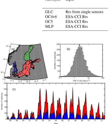
Table 1. Summary of the algorithms used in the validation analysis with the acronym used in this work along with the required input for each
of them. GLC stands for GlobColour, OC4v6 for Ocean Colour four-band algorithm (version 6), OC5 for Ocean Colour five-band algorithm, and MLP for multi-layer perceptron.
Acronym Input Chla Reference
algorithm
GLC Rrs from single sensors GSM Maritorena and Siegel (2005)
OC4v6 ESA-CCI Rrs OC4v6 Werdell (2010)
OC5 ESA-CCI Rrs OC5 Gohin et al. (2002)
MLP ESA-CCI Rrs MLP D’Alimonte et al. (2011)
98 99 00 01 02 03 04 05 06 07 08 09 10 11 12 0 20 40 60 80 100 120 Year N u m b e r o f m a tc h u p s
0.1 1 10 100 0 50 100 150 200 250 300
CHL in situ (mg m )-3
N u m b e r o f m a tc h u p s 5° E 10°
E 15°
E 20° E 25° E 30° E 55° N 60° N 65° N (a) (c) (b)
Figure 1. (a) Spatial distribution of the 4492 in situ stations used in
the matchup analysis (see Sect. 3.1) along with the partition of the area of study. The Skagerrak and Kattegat is highlighted in blue with 1456 matchup points, Central Baltic is highlighted in red with 2922 matchup points, and the Gulf of Bothnia is green with 114 stations. Temporal station distribution is also shown using the same colour code (b). The frequency distribution of the entire in situ Chlais shown in panel (c).
Similarly, to ensure representativeness of the data in the case of Chl a stratification, only stations with the upper-most reading shallower than 2 m were retained for the anal-ysis. The spatial location of matchup stations is shown in Fig. 1a. Although covering the entire Baltic region, data are not uniformly distributed, as the data set is built from dif-ferent sources, in which individual institutions and agencies are interested in specific zones. The number of matchups in-creases significantly when both MODIS-Aqua and MERIS started to operate in 2002 (Fig. 1b), thus providing further ev-idence of the utility of merging different sensors for oceano-graphic research. The Chlain situ data set used in the follow-ing sections of this work is log-normally distributed around the mean value of∼2.46 mg m−3and spanning from 0.1 to
77 mg m−3 (Fig. 1c). Fleming and Kaitala (2006) reported
Chlavalues 7–12 mg m−3in the northern Baltic Proper
dur-ing the sprdur-ing bloom. Our gathered in situ matchup data
set during April in the northern Baltic Proper (35 samples) shows Chla to range from 1.39 to 14.7 mg m−3, consistent
with these previous findings. 2.3 Statistical evaluation
Satellite Chla was extracted from single pixels without fur-ther spatial windowing. To calculate the mean bias and the rms we applied a decimal logarithm transformation to the Chladata, and returned to percentage linear scale:
bias=h10N1
PN
i=1(yi−xi)−1 i
·100 (1)
rms=
10N1 q
PN
i=1(yi−xi) 2
−1
·100, (2)
wherexiandyiare the log10-transformed in situ and satellite Chla, respectively.N is the number of matchups. The best linear fits were found using the log-transformed Chla. The corresponding coefficient of determination (R2), slope (m), and intercept (n) are also presented. The whole area was di-vided into regions with expected bio-optical differences (see Fig. 1a). The number of observations available from the Gulf of Bothnia is very limited, so the statistical information that can be derived from the regressions must be interpreted with caution. Nevertheless, results are presented for completeness. Thepvalue of the regressions was 0 for all regions except for the Gulf of Bothnia, where it wasp< 10−3.
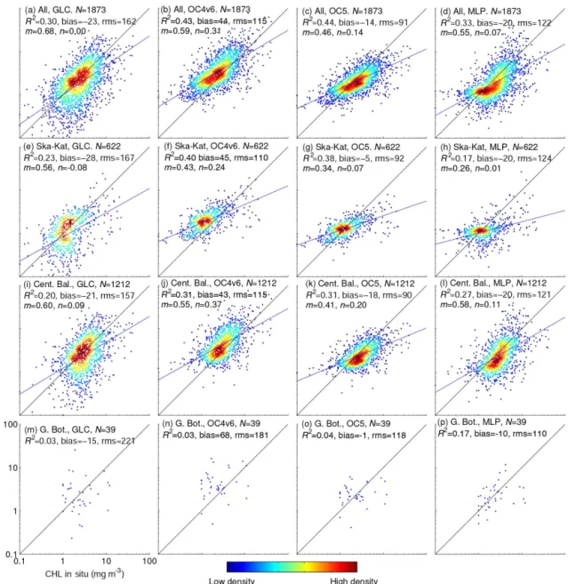
Figure 2. Density scatter plots of in situ vs. satellite-retrieved Chlafor all algorithms providing meaningful values. The line of best fit (blue) and that of equal value (black) are superimposed, with relevant statistics.
3 Results and discussion 3.1 Matchups
In general, satellite and in situ data show modest agreement in the Baltic. This can be intuitively associated with both the non-full traceability of the methods used to assemble the in situ data set and the satellite algorithms. MLP and GLC pro-vide poorR2and negative bias with respect to the in situ data. Results of OC4v6 (R2=0.43) are consistent with findings by Darecki and Stramski (2004). The positive bias of 44 % here (Fig. 2b) is smaller than 119 %, as found by Darecki and Stramski (2004), but still confirms OC4v6 to overestimate Chlain the Baltic Sea. OC4v6 matches the in situ data
bet-ter for high Chla, but tends to saturate for low values. OC5 has similar linearity (R2=0.44) but significantly improves in terms of bias (−14 %) with respect to OC4v6. Besides the similarR2, we noticed graphical similarities between the scatter plots of OC4v6 and OC5. Guided by this hint, we per-formed a linear regression in log form between OC4v6 and OC5 satellite-derived Chla (not shown). Regression analy-sis revealed a very high linear dependence (R2=0.97), al-though the relationship is more complex in theory (Gohin et al., 2002), and this will have implications for the rest of this work (see below).
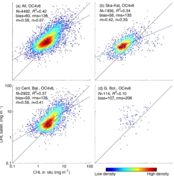
de-Figure 3. Density scatter plots of in situ vs. satellite-retrieved Chla
for the OC4v6 algorithm. The best linear regression (blue) and the line of equal value (black) are superimposed, with relevant statistics.
grades in the Skagerrak and Kattegat (Fig. 2h) with respect to the central Baltic Sea (Fig. 2l). MLP was calibrated with data only inside the Baltic Sea, and not in the Skagerrak and Kattegat (D’Alimonte et al., 2012, Fig. 2d). It appears then that such algorithm design is highly dependent on the cali-bration data. GLC always performs the worst in all regions, and the scatter plots look like undefined clouds, which is best highlighted by the large rms errors. OC4v6 displays simi-lar statistics at both sides of the Danish Strait, although the slope of the regression line decreases towards the Skagerrak and Kattegat. In each region, OC4v6 overestimates Chlaby more than 40 %. The behaviour of OC5 is always in accor-dance with OC4v6, with a shifted bias, given the very high correlation between the two. Due to the much simpler appli-cability of OC4v6 and its wider diffusion in the community, the following analysis will be based on OC4v6.
The matchup analysis is repeated here with the same con-ditions, including the definition and removal of the out-liers, but only for OC4v6. Only 22 matchups were discarded (< 0.5 % of the data), with 17 due to overestimation (i.e. higher than 20 times the in situ counterpart). As mentioned, when the coincidence with the other algorithms is removed, the number of matchups increases to 4492, distributed as 1456 in the Skagerrak and Kattegat, 2922 in the Central Baltic and 114 in the Gulf of Bothnia. Figure 3 shows the corresponding density scatter plots and statistics. In gen-eral, the interpretation from Fig. 2 still holds, with the big-ger size of the matchup data set providing increased confi-dence level of the derived statistics. However, since the
ad-Figure 4. Upper left panels, in black: best linear fits (slope
m and intercept n) of 1000 randomly chosen calibration
data sets (Ncal=2246, x axis) of log10 (CHL ain situ) vs.
log10(CHLaOC4v6). Lower left panel: application of all 1000 (m, n) pairs to the OC4v6 vs. in situ scatter cloud. In red, slope and intercept for the whole data set, as shown in Fig. 3a. In green, aver-age of the 1000 calibration results. Right panels, in black: statistics when applying eachmandnpair from the left side to the comple-mentary validation data sets (Nval=2246,x axis). These are the
coefficient of determination, bias (Eq. 1), and rms (Eq. 2). Same statistics found for the whole data set, as shown in Fig. 3a, are in red. The average of the 1000 validation results is in green.
ditional data were previously discarded (not used to produce Fig. 2), it is not surprising that the latter statistics did de-grade (R2=0.43, bias=72 %, RMSE=151 %, m=0.57, n=0.41, N =2619). The orders of magnitude of the un-certainties found here (Fig. 3) are in line with those available from the literature (Darecki and Stramski, 2004) even consid-ering the wider space and time distribution of the data (both in situ and satellite) used here.
3.2 Validation
When the regression coefficients are used to recalibrate ex-isting algorithms, the validity and robustness of the matchup statistics needs to be validated against independent data. Starting from the matchups for OC4v6 alone (Fig. 3a), we performed a sensitivity study to test the data set homogene-ity by a bootstrapping-like assessment (Efron, 1979) as used in recent validation exercises (Brewin et al., 2013). The whole data set (N =4492) was partitioned 1000 times into two randomly chosen halves: calibration (Ncal=2246) and
validation (Nval=2246). Each calibration data set is used
–2 –1.5 –1 –0.5 0 0.5 1 1.5 2 0
0.5 1 1.5 2 2.5x 10
5
log
10(CHLOC4v6corr) – log10(CHL in situ)
Mean: µ = 2.24 x 10⁻⁴ Standard deviation: σ = 0.4582
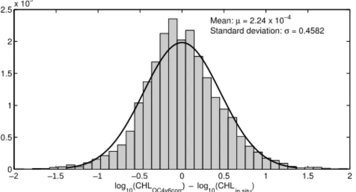
Figure 5. Histogram of the absolute error between OC4v6corrand
in situ Chla, both in logarithmic form. Associated mean and stan-dard deviation are also shown and used to compute a relevant fitted Gaussian distribution (black line).
Fig. 4) are almost equal to those found when the whole data set is used (m=0.5845 and n=0.3656, red lines in Fig. 4). Moreover, the dispersion is very small with the co-efficient of variation being 2.07 % when computed over the slopes and 1.38 % over the intercepts. As for the valida-tion statistics, their mean values (graphically shown in green in Fig. 4)R2=0.4236, bias=59.55 %, rms=136.13 % are very similar to those obtained for the whole data set (Fig. 3a, R2=0.4241, bias=59.53 %, rms=136.19 %).
3.3 Algorithm regional calibration
Efficient and useful algorithm regionalization needs appro-priate bio-optical in situ data. Unfortunately, the Baltic lacks such a publicly available in situ data set that therefore pre-vents a canonical regionalization. This, together with the high confidence level associated with the described statistics and in view of obtaining an unbiased proxy for Chla, with the available data, prompts the use of the computed coeffi-cients (mandnin Fig. 4) for recalibrating OC4v6, as fol-lows:
log10(CHLaOC4v6corr)=
log10(CHLaOC4v6)−n
m . (3)
Errors between Eq. (3) and the complementary in situ val-idation matchups were calculated. Each of the 1000 cho-sen combinations generated a vector of errors with length Nval=2246. Their accumulation led to a total of 2 246 000
error estimates, whose distribution is shown in Fig. 5, to-gether with the fitted Gaussian curve. The recalibration in Eq. (3) removed the bias, resulting in a zero-centred error distribution. It is worth reminding that, within the calibration and validation exercises, the two data sets are independent. The standard deviation (σ=0.4582) includes all errors not taken into account by the system, i.e. atmospheric noise, er-rors in the in situ measurements and, most of all, the limited suitability of algorithms such as OC4v6.
The symmetric and zero-centred error distribution (Fig. 5) obtained with the application of Eq. (3) within the bootstrapping-like assessment warrants a high level of con-fidence when basin averages are calculated; all the errors at the level of individual pixels are expected to cancel out when a horizontal (pixel-wise) average is performed over a large region. Although the former statement implies that the statis-tical properties of the matchup data set can be extrapolated to the whole Baltic area, the good spatial and temporal cover-age of the former (see Fig. 1) helps to support this argument. From this point, we defined the algorithm OC4v6corrthrough Eq. (3), with the coefficients (m=0.5884,n =0.3751) of Fig. 3a. This enabled the bias to be removed. Neverthe-less, rms was altered, rising to 187 %, in agreement with σ=0.4582 in Fig. 5 through Eq. (2). The mathematical
ex-planation of the latter relationship is that the rms and the stan-dard deviation of a zero-mean distribution are equal.
Among all regions in which the Baltic Area has been di-vided, Fig. 3 highlights different best linear fits. Given the coefficients of variation 2.07 and 1.38 % for the slope and intercept, respectively, found in the bootstrapping assess-ment, the coefficients in Fig. 3 are significantly different. If OC4v6 is linearly adjusted with Eq. (3), the coefficients must be different for each region in particular and equal to those found in Fig. 3. Therefore, for the Skagerrak and Kat-tegat, they were set to 0.4212 and 0.3027, respectively, for mandn. Due to the lack of data, the stations in the Gulf of Bothnia were aggregated to those of the Central Baltic. Re-sulting statistics for these two regions were almost equal to those of the Central Baltic alone:R2=0.35, bias=60.45 %,
rms=138.64 %,m=0.5632, andn=0.4206. These linear
coefficients were applied to recalibrate OC4v6 for the Cen-tral Baltic and the Gulf of Bothnia. Even if the same algo-rithm was used, results are presented separately for the two basins.
3.4 Satellite-derived basin averages
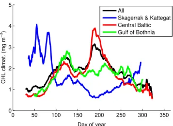
Horizontally averaged Chl a for OC4v6corr was computed only for images with a minimum number of 1000 valid pix-els. The entire Baltic has 21 424 pixels, with the Gulf of Bothnia contributing with 5750 pixels, the Skagerrak and Kattegat with 2625 pixels, and the Central Baltic with 13 049 pixels. One thousand pixels correspond to 5, 17, 38, and 7 % of their respective surfaces. Chla dynamics strongly varies among regions at both seasonal (Fig. 6) and interannual timescales (Supplement). In the Skagerrak and Kattegat, the dynamics consist of intermittent growth periods in late winter (up to∼4 mg m−3)and a small bloom in spring, reaching a
minimum in summer (∼0.5 mg m−3), consistent with other
works (Edelvang et al., 2005) . In the Gulf of Bothnia, the overall range of Chla variability is limited to∼2 mg m−3
(0.7–2.8 mg m−3) with minima in winter and a series of
0 50 100 150 200 250 300 350 0
1 2 3 4 5
Day of year
C
H
L
c
lim
a
t.
(
m
g
m
–3
)
All
Skagerrak & Kattegat Central Baltic Gulf of Bothnia
Figure 6. Chladaily climatology. For any given day of the year, the average was computed only if data for a minimum of 6 years were available. Plots of individual time series with their associated standard deviation bars can be found in the Supplement. To improve the plot readability, all time series were smoothed with a 1-week moving average.
et al., 2015). Given the prolonged winter darkness, the length of this data time series is shorter than those from the other regions. Moreover, in winter the Gulf of Bothnia is normally ice covered and some ice remains in the northern part until May; thus, not the entire domain contributed to the displayed Chla. A non-trivial point is that this time series has to be interpreted with caution due to lack of a significant num-ber of data for specific calibration in this area. In the Cen-tral Baltic, the dynamics is completely different. Two distinct Chla maxima are appreciable (Reissmann et al., 2009): the first one peaks at the end of April, reaching∼2.5 mg m−3,
which is at the lower end of the variability previously ob-served by Schneider et al. (2006); the intensity of the second peak, in mid-July, (∼4.6 mg m−3)is consistent with previous
observations in the area (Schneider et al., 2006), and allows it to steadily decrease and reach a minimum in winter. The dy-namics of the entire domain (black line in Fig. 6) are clearly dominated by the Central Baltic due to its major weight in terms of area coverage. The summer bloom that occurs in the Central Baltic is known to occur due to cyanobacteria taking advantage of the milder weather conditions and of the increased water temperature. As cyanobacteria can form sur-face scum, it is worth questioning whether such data would be masked during the operational image processing. A previ-ously documented mild cyanobacteria bloom on 11 July 2010 was visible from space via qualitative RGB image. Here, surface accumulations were not observed (SMHI, 2010). To assess whether the standard processing is also able to pro-vide reliable observations in these conditions, MODIS-Aqua Level-1A was downloaded and processed to L2 using the same settings used to produce the CCI input data. Figure 7a shows the Central Baltic blooming also in the areas identified
as cyanobacteria by the SeaDAS Level-2 flag TURBIDW (Fig. 7b) used to discriminate the accumulation of cyanobac-teria (Kahru and Elmgren, 2014). During summer 2005, the Baltic experienced the second largest cyanobacteria bloom (Kahru and Elmgren, 2014) that covered 25 % of the entire domain (183 000 km2). As for the 2010 bloom – and apart from the small area classified as too bright in the north Baltic Proper (in light grey in Fig. 7c and d) – the standard pro-cessing demonstrated its ability to provide valid data also under these conditions. Therefore, the data used here appear suitable for the study of phytoplankton dynamics throughout the year, even during cyanobacteria bloom events, when only a negligible percentage of pixels is affected by atmospheric correction failures (Kahru and Elmgren, 2014).
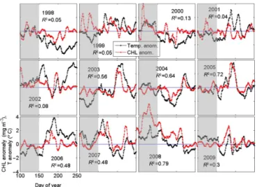
Figure 6 shows that the strongest signal in the Cen-tral Baltic is given by the summer bloom. Cyanobacteria-like species are known to bloom under warm and calm weather conditions (Ploug, 2008). High sea-surface temper-ature (SST) is known to enhance the growth of cyanobac-teria, both directly through higher growth rates, and indi-rectly by increasing the stability of the water column to allow cyanobacteria to take advantage of their buoyancy regulation ability (Ibelings et al., 1991). Analogously, cyanobacteria were demonstrated to provide positive feedbacks to the sur-face temperature by absorbing the incoming radiation (Kahru et al., 1993). It is then reasonable to investigate whether Chla and SST covary over the Central Baltic during summer. In the specific context of this cross-correlation analysis, we are implicitly assuming that both SST and Chlarespond to the calm weather conditions with the same time lag. For this mat-ter, daily-average SST data (1998–2009) over the Baltic Sea were downloaded from the CMEMS website. The SST data set is the merged product from the sensors AVHRRs (series 7, 9, 11, 14, 16, 17, 18), Envisat ATSR1 and ATSR2, and the AATSR (see CMEMS (2015) for details and the Supplement for their basin-average time series). Both Chlaand SST data time series were deseasonalized by computing the anoma-lies with respect to their climatologies, which were used as input for the cross-correlation analysis. Figure 8 shows the two time series anomalies along with correlation values com-puted over the summer period (between the Julian days 150 and 250) for all years for which SST was available. Prior to the correlation analysis, the Chl a anomaly time series was further smoothed with a 1-week moving average. Here, the basic underlying assumption is that warm waters, as a proxy of calm weather conditions, can explain the dynamics of cyanobacteria. Thus, when cyanobacteria do represent a high fraction (in terms of their space and time presence) of the Chlasignal, the correlation is expected to be high, and vice versa.
Figure 7. MODIS Level-1A of 11 July 2010 (a, b) and 2005 (c, d) were downloaded from the OBPG website (Ocean
Biol-ogy Processing Group, oceancolor.gsfc.nasa.gov) and processed to Level-2 using the standard settings within SeaDAS version 7.3 (seadas.gsfc.nasa.gov). Kahru and Elmgren (2014) recently identi-fied the presence of cyanobacteria accumulating on the sea surface using the SeaDAS Level-2 flag TURBIDW (“turbid water”) when the flag MAXAERITER (“maximum aerosol iterations”) is turned off within the Level-1 to Level-2 processing. Here, Chlaimages without (a, c) and with (b, d) the application of the TURBIDW flag are shown; pixels affected by TURBIDW are coloured black. As mentioned by Kahru and Elmgren (2014), the MAXAERITER flag is, by default, turned on within the NASA standard process-ing (e.g. the same used here). A light grey area (c, d) in the north-western Baltic Proper is perceived by the operational processing as too bright (i.e. masked as MAXAERITER) and not processed.
their climatological values. Generally, during the second half of the time series, from 2003 on, the correlation appears to be tighter. The causes of the dynamics shown are undoubt-edly complex, involving considerations on the circulation and the peculiar biogeochemistry of the basin (Reissmann et al., 2009). Nevertheless, this article is focused on the remote-sensing aspect and the intensity of the cyanobacteria bloom appears to depend on the timing of the summer temperature peak: although 2004 had a high SST peak, such a peak hap-pened late in the season (10 August), which appeared un-favourable for cyanobacteria growth. On the contrary, years 2002, 2003, 2005, and 2006 had SST peaks of similar or lower intensity but much earlier in the season. Instead, 2001 displayed two marked positive SST anomalies that were only
Figure 8. Time series of the Chlaand SST anomalies with respect to their climatologies, over the Central Baltic. The reference value 0 is also displayed. Shaded areas indicate the part of the time series not used for the computation of the cross-correlation coefficient, which is indicated on each year. Full size plots of individual years can be found in the Supplement.
mildly followed by Chla anomalies. Despite the Chla and SST anomalies being poorly correlated during 1998 (Fig. 8), they were both negative. This suggests that in that year, the cyanobacteria bloom, generally dominating the summer sig-nal in the Central Baltic, was only partially contributing to the overall dynamics. This is clearly documented in Kahru and Elmgren (2014), who found the fraction of cyanobacte-ria accumulations (FCA) of only 6 % in 1998, which is the ratio of the number of pixels classified as cyanobacteria to the number of cloud-free sea-surface views during the period July–August.
4 Conclusions
A 15-year merged multi-sensor daily data set of satellite-derived Chlacontains very valuable information for ecolog-ical studies, if information is properly processed. Matchup analysis was undertaken with the largest in situ database ever used for calibration and validation purposes over the Baltic region. Standard algorithms proved to be easy to apply but, in the Baltic Sea, required further adjustments before an un-biased estimation of the basin-average Chl a was obtained. Our derived time series take advantage of the independence of the error added by other water constituents and additional sources. The error distribution of the Chla estimates, when averaging over a large number of observations, tends to zero, thus demonstrating that more accurate observations can be achieved when averaging over large areas.
The OC4v6corr-derived climatology in the Skagerrak and Kattegat revealed strong productivity in winter and a rather inactive summer. However, it should be noted that the blue– green Chl a algorithms are not optimal for the coccol-ithophore detection (Gordon et al., 2001), commonly ob-served in this area. In the Gulf of Bothnia, Chl a exhibits a single bloom during spring and experiences lower variabil-ity than the Skagerrak and Kattegat regions or the Central Baltic. In the latter region, the productivity in late fall, winter, and early spring is severely inhibited. A first growth period with a maximum at the end of April is detected, followed by a stronger summer bloom peaking in the second week of July. The summer bloom in the Central Baltic constitutes the most intense signal found in this work, and is attributed to cyanobacteria-like species. Chlaand SST anomaly time se-ries were cross-correlated to assess the cyanobacteria con-tribution to the overall Chla dynamics during the summer period of the Central Baltic. For example, the exceptionally warm winter 2007/2008 triggered an intense spring bloom in 2008 that also altered the normal dynamics throughout the year.
The Baltic region is widely recognized as a challenging test bed for ocean colour remote sensing. The interfering CDOM at blue wavelengths suggests that better Chla algo-rithms should use red and NIR bands, like the fluorescence line height or the maximum chlorophyll index algorithms (Odermatt et al., 2012, Fig. 1). Most of the Baltic Chla val-ues range between∼1 and 10 mg m−3and are at the lower
part of the retrievable concentrations, by these algorithms (Odermatt et al., 2012, Fig. 1). These algorithms are only applicable to the archived MERIS data (2002–2012). The Ocean and Land Colour Instrument, on-board the Sentinel-3 will provide continuity with MERIS and the algorithms will be adapted. The addition of the 400 nm band will expectedly aid in the separation of the CDOM contribution, given that proper atmospheric correction is achieved.
The Supplement related to this article is available online at doi:10.5194/os-12-379-2016-supplement.
Acknowledgements. The research leading to these results has
received funding from the European Union Seventh Framework Programme through HORIZON 2020 under grant agreement no. 210129802 (Copernicus Marine Environment Monitoring Service). Seadatanet, HELCOM, and NOAA along with all single contributors are thanked for the in situ data and CMEMS, ESA-CCI, and GlobColour for the satellite data. Vega Forneris is thanked for technical support and Vittorio Brando for suggestions on the manuscript. Two anonymous reviewers are thanked for their comments and suggestions.
Edited by: H. Bonekamp
References
Attila, J., Koponen, S., Kallio, K., Lindfors, A., Kaitala, S., and Ylöstalo, P.: MERIS Case II water processor comparison on coastal sites of the northern Baltic Sea, Remote Sens. Environ., 128, 138–149, doi:10.1016/j.rse.2012.07.009, 2013.
Berthon, J.-F. and Zibordi, G.: Optically black waters in the northern Baltic Sea, Geophys. Res. Lett., 37, L09605, doi:10.1029/2010GL043227, 2010.
Brewin, R. J. W., Sathyendranath, S., Müller, D., Brockmann, C., Deschamps, P.-Y., Devred, E., Doerffer, R., Fomferra, N., Franz, B., Grant, M., Groom, S., Horseman, A., Hu, C., Krasemann, H., Lee, Z., Maritorena, S., Mélin, F., Peters, M., Platt, T., Regner, P., Smyth, T., Steinmetz, F., Swinton, J., Werdell, J., and White Iii, G. N.: The Ocean Colour Climate Change Initiative: III, A round-robin comparison on in-water bio-optical algorithms, Remote Sensing of Environment, Volume 162, 1 June 2015, Pages 271– 294, ISSN 0034–4257, doi:10.1016/j.rse.2013.09.016, 2013. Carstensen, J., Klais, R., and Cloern, J. E.: Phytoplankton
blooms in estuarine and coastal waters: Seasonal patterns and key species, Estuar. Coast. Shelf S., 162, 98–109, doi:10.1016/j.ecss.2015.05.005, 2015.
D’Alimonte, D., Zibordi, G., Berthon, J. F., Canuti, E., and Ka-jiyama, T.: Bio-optical algorithms for European seas: Perfor-mance and applicability of neural-net inversion schemes, Joint research Centre, IspraJRC66326, 2011.
D’Alimonte, D., Zibordi, G., Berthon, J.-F., Canuti, E., and Ka-jiyama, T.: Performance and applicability of bio-optical algo-rithms in different European seas, Remote Sens. Environ., 124, 402–412, doi:10.1016/j.rse.2012.05.022, 2012.
Darecki, M. and Stramski, D.: An evaluation of MODIS and SeaW-iFS bio-optical algorithms in the Baltic Sea, Remote Sens. Envi-ron., 89, 326–350, doi:10.1016/j.rse.2003.10.012, 2004. Edelvang, K., Kaas, H., Erichsen, A. C., Alvarez-Berastegui, D.,
Bundgaard, K., and Jørgensen, P. V.: Numerical modelling of phytoplankton biomass in coastal waters, J. Marine Syst., 57, 13– 29, doi:10.1016/j.jmarsys.2004.10.003, 2005.
ESA-OC-CCI: Product User Guide: http://www.
esa-oceancolour-cci.org/?q=webfm_send/318 (last access:
1 February 2016), 2014.
Fleming, V. and Kaitala, S.: Phytoplankton Spring Bloom Inten-sity Index for the Baltic Sea Estimated for the years 1992 to 2004, Hydrobiologia, 554, 57–65, doi:10.1007/s10750-005-1006-7, 2006.
Gohin, F., Druon, J. N., and Lampert, L.: A five channel chlorophyll concentration algorithm applied to SeaWiFS data processed by SeaDAS in coastal waters, Int. J. Remote Sens., 23, 1639–1661, doi:10.1080/01431160110071879, 2002.
Gordon, H. R., Boynton, G. C., Balch, W. M., Groom, S. B., Har-bour, D. S., and Smyth, T. J.: Retrieval of coccolithophore calcite concentration from SeaWiFS Imagery, Geophys. Res. Lett., 28, 1587–1590, doi:10.1029/2000GL012025, 2001.
HELCOM: Thematic Report on Validation of Algorithms for Chlorophyll a Retrieval from Satellite Data in the Baltic Sea Area, Helsinki Commission-HELCOM, Ispra94, 2004.
Ibelings, B. W., Mur, L. R., and Walsby, A. E.: Diurnal changes in buoyancy and vertical distribution in populations of Mi-crocystisin two shallow lakes, J. Plankton Res., 13, 419–436, doi:10.1093/plankt/13.2.419, 1991.
IOCCG: Ocean-colour data merging, IOCCG, Dartmouth,
Canada6, 2007.
Kahru, M. and Elmgren, R.: Multidecadal time series of satellite-detected accumulations of cyanobacteria in the Baltic Sea, Biogeosciences, 11, 3619–3633, doi:10.5194/bg-11-3619-2014, 2014.
Kahru, M., Savchuk, O. P., and Elmgren, R.: Satellite measurements of cyanobacterial bloom frequency in the Baltic Sea: interan-nual and spatial variability, Mar. Ecol.-Prog. Ser., 343, 15–23, doi:10.3354/meps06943, 2007.
Kratzer, S., Brockmann, C., and Moore, G.: Using MERIS full resolution data to monitor coastal waters – A case study from Himmerfjärden, a fjord-like bay in the north-western Baltic Sea, Remote Sens. Environ., 112, 2284–2300, doi:10.1016/j.rse.2007.10.006, 2008.
Larsson, K., Hajdu, S., Kilpi, M., Larsson, R., Leito, A., and Lyngs, P.: Effects of an extensive Prymnesium polylepis bloom on breeding eiders in the Baltic Sea, J. Sea Res., 88, 21–28, doi:10.1016/j.seares.2013.12.017, 2014.
Majaneva, M., Rintala, J.-M., Hajdu, S., Hällfors, S., Häll-fors, G., Skjevik, A.-T., Gromisz, S., Kownacka, J., Busch, S., and Blomster, J.: The extensive bloom of alternate-stage Prymnesium polylepis (Haptophyta) in the Baltic Sea dur-ing autumn–sprdur-ing 2007–2008, Eur. J. Phycol., 47, 310–320, doi:10.1080/09670262.2012.713997, 2012.
Maritorena, S. and Siegel, D. A.: Consistent merging of satellite ocean color data sets using a bio-optical model, Remote Sens. Environ., 94, 429–440, doi:10.1016/j.rse.2004.08.014, 2005. Maritorena, S., d’Andon, O. H. F., Mangin, A., and Siegel, D. A.:
Merged satellite ocean color data products using a bio-optical model: Characteristics, benefits and issues, Remote Sens. Envi-ron., 114, 1791–1804, doi:10.1016/j.rse.2010.04.002, 2010.
Mélin, F. and Vantrepotte, V.: How optically diverse is the coastal ocean?, Remote Sens. Environ., 160, 235–251, doi:10.1016/j.rse.2015.01.023, 2015.
Morel, A. and Berthon, J.-F.: Surface pigments, algal biomass pro-files, and potential production of the euphotic layer: Relation-ships reinvestigated in view of remote-sensing applications, Lim-nol. Oceanogr., 34, 1545–1562, 1989.
Product User Guide: http://www.globcolour.info/CDR_Docs/
GlobCOLOUR_PUG.pdf (last access: 1 February 2016), 2015. Product User Manual for Baltic Sea Physical Reanalysis
Products: http://marine.copernicus.eu/documents/PUM/
CMEMS-OC-PUM-009-ALL.pdf (last access: 1 February 2016), 2015.
Odermatt, D., Gitelson, A., Brando, V. E., and Schaepman, M.: Re-view of constituent retrieval in optically deep and complex wa-ters from satellite imagery, Remote Sens. Environ., 118, 116– 126, doi:10.1016/j.rse.2011.11.013, 2012.
Pierson, D. C., Kratzer, S., Strömbeck, N., and Håkansson, B.: Relationship between the attenuation of downwelling irradi-ance at 490 nm with the attenuation of PAR (400 nm–700 nm) in the Baltic Sea, Remote Sens. Environ., 112, 668–680, doi:10.1016/j.rse.2007.06.009, 2008.
Ploug, H.: Cyanobacterial surface blooms formed by Aphani-zomenon sp. and Nodularia spumigena in the Baltic Sea: Small-scale fluxes, pH, and oxygen microenvironments, Limnol. Oceanogr., 53, 914–921, doi:10.4319/lo.2008.53.3.0914, 2008. Reinart, A. and Kutser, T.: Comparison of different satellite sensors
in detecting cyanobacterial bloom events in the Baltic Sea, Re-mote Sens. Environ., 102, 74–85, doi:10.1016/j.rse.2006.02.013, 2006.
Reissmann, J. H., Burchard, H., Feistel, R., Hagen, E., Lass, H. U., Mohrholz, V., Nausch, G., Umlauf, L., and Wiec-zorek, G.: Vertical mixing in the Baltic Sea and consequences for eutrophication – A review, Prog. Oceanogr., 82, 47–80, doi:10.1016/j.pocean.2007.10.004, 2009.
Schneider, B., Kaitala, S., and Maunula, P.: Identification and quan-tification of plankton bloom events in the Baltic Sea by contin-uous pCO2 and chlorophyll a measurements on a cargo ship, J. Marine Syst., 59, 238–248, doi:10.1016/j.jmarsys.2005.11.003, 2006.
Siegel, H. and Gerth, M.: Optical Remote Sensing Applications in the Baltic Sea, in: Remote Sensing of the European Seas, edited by: Barale, V. and Gade, M., Springer Netherlands, Dordrecht, 91–102, 2008.
SMHI: A mild algal bloom in 2010: http://www.smhi.se/en/ news-archive/a-mild-algal-bloom-in-2010-1.12999 (last access: 1 February 2016), 2010.
Wasmund, N. and Uhlig, S.: Phytoplankton trends in the Baltic Sea, ICES J. Mar. Sci., 60, 177–186, doi:10.1016/s1054-3139(02)00280-1, 2003.