Biogeochemical processes and buffering capacity concurrently affect acidification in a seasonally hypoxic coastal marine basin

(1)

BGD

11, 15827–15887, 2014

Acidification in a seasonally hypoxic

coastal basin

M. Hagens et al.

Title Page

Abstract Introduction

Conclusions References

Tables Figures

◭ ◮

Back Close

Full Screen / Esc

Printer-friendly Version Interactive Discussion

Discussion

P

a

per

|

Discussion

P

a

per

|

Discussion

P

a

per

|

Discussion

P

a

per

|

Biogeosciences Discuss., 11, 15827–15887, 2014 www.biogeosciences-discuss.net/11/15827/2014/ doi:10.5194/bgd-11-15827-2014

This discussion paper is/has been under review for the journal Biogeosciences (BG). Please refer to the corresponding final paper in BG if available.

Biogeochemical processes and bu

_ff

ering

capacity concurrently a

_ff

ect acidification

in a seasonally hypoxic coastal marine

basin

M. Hagens1, C. P. Slomp1, F. J. R. Meysman2,3, D. Seitaj2, J. Harlay4,*, A. V. Borges4, and J. J. Middelburg1

1

Department of Earth Sciences, Faculty of Geosciences, Utrecht University, the Netherlands

2

Department of Ecosystem Studies, Royal Netherlands Institute for Sea Research, Yerseke, the Netherlands

3

Department of Analytical, Environmental and Geochemistry, Faculty of Science, Vrije Universiteit Brussel, Belgium

4

Chemical Oceanography Unit, University of Liège, Belgium

*

now at: Department of Oceanography, University of Hawaii, USA

Received: 13 October 2014 – Accepted: 28 October 2014 – Published: 18 November 2014

Correspondence to: M. Hagens (m.hagens@uu.nl)

(2)

BGD

11, 15827–15887, 2014

coastal basin

M. Hagens et al.

Title Page

Tables Figures

◭ ◮

Back Close

Full Screen / Esc

Discussion

P

a

per

|

Discussion

P

a

per

|

Discussion

P

a

per

|

Discussion

P

a

per

|

Abstract

Coastal areas are impacted by multiple natural and anthropogenic processes and ex-perience stronger pH fluctuations than the open ocean. These variations can weaken or intensify the ocean acidification signal induced by increasing atmosphericpCO₂. The development of eutrophication-induced hypoxia intensifies coastal acidification, since

5

the CO2 produced during respiration decreases the buffering capacity of the hypoxic

bottom water. To assess the combined ecosystem impacts of acidification and hypoxia, we quantified the seasonal variation in pH and oxygen dynamics in the water column of a seasonally stratified coastal basin (Lake Grevelingen, the Netherlands).

Monthly water column chemistry measurements were complemented with estimates

10

of primary production and respiration using O2 light-dark incubations, in addition to

sediment-water fluxes of dissolved inorganic carbon (DIC) and total alkalinity (TA). The resulting dataset was used to set up a proton budget on a seasonal scale.

Temperature-induced seasonal stratification combined with a high community respi-ration was responsible for the depletion of oxygen in the bottom water in summer. The

15

surface water showed strong seasonal variation in process rates (primary production, CO2 air–sea exchange), but relatively small seasonal pH fluctuations (0.46 units on

the total hydrogen ion scale). In contrast, the bottom water showed less seasonality in biogeochemical rates (respiration, sediment–water exchange), but stronger pH fluc-tuations (0.60 units). This marked difference in pH dynamics could be attributed to a

20

substantial reduction in the acid-base buffering capacity of the hypoxic bottom water in the summer period. Our results highlight the importance of acid-base buffering in the pH dynamics of coastal systems and illustrate the increasing vulnerability of hypoxic, CO2-rich waters to any acidifying process.

(3)

BGD

11, 15827–15887, 2014

coastal basin

M. Hagens et al.

Title Page

Tables Figures

◭ ◮

Back Close

Full Screen / Esc

Discussion

P

a

per

|

Discussion

P

a

per

|

Discussion

P

a

per

|

Discussion

P

a

per

|

1 Introduction

The absorption of anthropogenic carbon dioxide (CO2) has decreased the average pH

of open ocean surface water by circa 0.1 unit since the Industrial Revolution (Orr et al., 2005). In coastal areas, the problem of ocean acidification is more complex, as seawa-ter pH is influenced by various natural and anthropogenic processes other than CO2

5

uptake (Borges and Gypens, 2010; Duarte et al., 2013; Hagens et al., 2014). As a re-sult, the signal of CO₂-induced acidification may not be readily discernable in coastal systems, as time series of pH show high variations at diurnal, seasonal and decadal time scales (e.g., Hofmann et al., 2011; Wootton and Pfister, 2012). One major anthro-pogenic process impacting coastal pH is eutrophication (Borges and Gypens, 2010;

10

Provoost et al., 2010; Cai et al., 2011). Enhanced inputs of nutrients lead to higher rates of both primary production and respiration (Nixon, 1995), thereby increasing the variability in pH on both the diurnal (Schulz and Riebesell, 2013) and seasonal scale (Omstedt et al., 2009). Moreover, when primary production and respiration are not bal-anced, they can lead to longer-term changes in pH at rates which can strongly exceed

15

the expected pH decrease based on rising atmospheric CO₂ (Borges and Gypens, 2010). The direction of this eutrophication-induced pH change depends on the sign of the imbalance and the resulting pH trend can be sustained for decades (Provoost et al., 2010; Duarte et al., 2013).

A well-known effect of eutrophication is the development of hypoxia in coastal bottom

20

waters (Diaz and Rosenberg, 2008). Such bottom-water oxygen (O2) depletion occurs

when the O₂consumption during respiration exceeds the supply of oxygen-rich waters and typically develops seasonally as a result of summer stratification and enhanced biological activity. As respiration of organic matter produces CO2at a rate proportional

to O₂consumption (Redfield et al., 1963), it follows that zones of low O₂are also zones

25

(4)

BGD

11, 15827–15887, 2014

coastal basin

M. Hagens et al.

Title Page

Tables Figures

◭ ◮

Back Close

Full Screen / Esc

Discussion

P

a

per

|

Discussion

P

a

per

|

Discussion

P

a

per

|

Discussion

P

a

per

|

seasonal time scales (Frankignoulle and Distèche, 1984; Melzner et al., 2012), where the diurnal variability may be of similar magnitude as the seasonal variability (Yates et al., 2007). Primary production and respiration are often spatially and temporally decoupled, as phytoplankton biomass is produced during spring blooms in the surface water, subsequently sinks, and is degraded with a time lag in the bottom water and

5

sediment. In seasonally stratified areas, this can lead to significant concomitant drops in bottom-water pH and O₂ in summer, as has been shown for the Seto Inland Sea (Taguchi and Fujiwara, 2010), the northern Gulf of Mexico and the East China Sea (Cai et al., 2011), the Bohai Sea (Zhai et al., 2012), the Gulf of Trieste (Cantoni et al., 2012), several estuarine bays across the northeastern US coast (Wallace et al., 2014), the

10

semi-enclosed Lough Hyne (Sullivan et al., 2014) and in areas just o_ffthe Changjiang Estuary (Wang et al., 2013).

Long-term trends in pH resulting from increased prevalence of bottom-water hy-poxia can be substantial compared to the pH trend resulting from anthropogenic CO₂ -induced acidification. Data from the Lower St. Lawrence Estuary indicates that the

15

decrease in bottom-water pH over the last 75 years is 4–6 times higher than can be explained by the uptake of anthropogenic CO₂ alone (Mucci et al., 2011). In Puget Sound, respiration currently accounts for 51–76 % of the decrease in subsurface water pH since pre-industrial times, although this fraction will likely decrease as atmospheric CO₂continues to increase (Feely et al., 2010). Model simulations for the northern Gulf

20

of Mexico show that the seasonal drop in bottom-water pH has increased in the Anthro-pocene because of a decline in its buffering capacity (Cai et al., 2011), an effect that is most pronounced in eutrophied waters at relatively high temperatures and salinities (Sunda and Cai, 2012).

The acid-base buffering capacity (β), also termed the buffer intensity or buffer factor,

25

is the ability of an aqueous solution to counteract changes in pH or proton (H+) concen-tration upon the addition of a strong acid or base (Morel and Hering, 1993; Stumm and Morgan, 1996). It is of great importance when considering the effect of biogeochemical processes on pH (Zhang, 2000; Soetaert et al., 2007; Hofmann et al., 2010a). A

(5)

BGD

11, 15827–15887, 2014

coastal basin

M. Hagens et al.

Title Page

Tables Figures

◭ ◮

Back Close

Full Screen / Esc

Discussion

P

a

per

|

Discussion

P

a

per

|

Discussion

P

a

per

|

Discussion

P

a

per

|

tem with a high acid-base buffering capacity is efficient in attenuating changes in [H+] and thus displays a relatively smaller net pH change compared to systems with a low

β. Thus, if two aqueous systems are exposed to the same biogeochemical processes at exactly the same rate, the system with the lower β will show pH excursions with larger amplitudes.

5

In the 21st century, seawater buffering capacity is expected to decline as a result of increasing CO2 and the subsequent decrease in pH (Egleston et al., 2010; Hofmann

et al., 2010a; Hagens et al., 2014). As a result, one would predict a greater seasonal pH variability (Frankignoulle, 1994; Egleston et al., 2010) and a more pronounced diurnal pH variability in highly productive coastal environments (Schulz and Riebesell, 2013;

10

Shaw et al., 2013), which may additionally be modified by ecosystem feedbacks (Jury et al., 2013). In seasonal hypoxic systems, model analysis predicts more pronounced fluctuations in bottom-water pH (Sunda and Cai, 2012). However, detailed studies of the effects of seasonal hypoxia on pH buffering and dynamics are currently lacking.

Here we present a detailed study of the pH dynamics and acid-base buffering

capac-15

ity in a temperate coastal basin with seasonal hypoxia (Lake Grevelingen). We quan-tify the impact of individual processes, i.e., primary production, community respiration, sediment effluxes and CO2air–sea exchange, on pH. From this, we construct a proton

budget that attributes proton production or consumption to these processes. Our aim is to quantify seasonal changes in the acid-base buffering capacity and elucidate their

20

importance for carbon cycling and pH dynamics in coastal hypoxic systems.

2 Methods

2.1 Site description

Lake Grevelingen, located in the southwestern delta area of the Netherlands, is a coastal marine lake with a surface area of 115 km2 and an average water depth

25

(6)

BGD

11, 15827–15887, 2014

coastal basin

M. Hagens et al.

Title Page

Tables Figures

◭ ◮

Back Close

Full Screen / Esc

Discussion

P

a

per

|

Discussion

P

a

per

|

Discussion

P

a

per

|

Discussion

P

a

per

|

gullies intersecting extended shallow areas; half of the lake is shallower than 2.6 m, and only 12.4 % of the lake is deeper than 12.5 m. In the main gully, several deep basins are present, which are separated from each other by sills. The deepest basin extends down to 45 m water depth. Originally, Lake Grevelingen was an estuary with a tidal range of about 2.3 m. A large flooding event in 1953 was the motive for the

con-5

struction of two dams. The Grevelingen estuary was closed offon the landward side in 1964 and on the seaward side in 1971. This isolation led to a freshening of the system, with vast changes in water chemistry and biology (Bannink et al., 1984). To counteract these water quality problems, a sluice extending vertically between 3 and 11 m depth was constructed on the seaward side in 1978 (Pieters et al., 1985). Exchange with

10

saline North Sea water has dominated the water budget since, resulting in the lake ap-proaching coastal salinity (29–32) and an estimated basin-wide water residence time of 229 days (Meijers and Groot, 2007). Upon intrusion, the denser North Sea water forms a distinct subsurface layer, which is then laterally transported into the lake. Yet it has been found that opening the sluice hardly affects water-column mixing (Nolte

15

et al., 2008) and the water quality problems sustain. Monthly monitoring carried out by the executive arm of the Dutch Ministry of Infrastructure and the Environment revealed that the main gully of Lake Grevelingen has experienced seasonal stratification and hypoxia since the start of the measurements in 1978, though differing in extent and intensity annually (Wetsteyn, 2011).

20

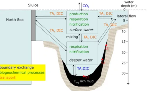
Throughout 2012, we performed monthly sampling campaigns onboard the R/V

Luctorexamining water column chemistry, biogeochemical rates and sediment–water exchange. Sampling occurred in the Den Osse Basin (maximum water depth 34 m; Fig. 1b), a basin located in the main gully of Lake Grevelingen. Two sills surround the basin at water depths of 10 and 20 m at the landward and seaward side, respectively.

25

Due to its bathymetry, particulate matter rapidly accumulates within the deeper parts of the basin (sediment accumulation rate>2 cm yr−1; Malkin et al., 2014). The surface area and total volume of the Den Osse Basin have been estimated at 649×104m2and

655×105m3, respectively (Pieters et al., 1985), resulting in an average water depth

(7)

BGD

11, 15827–15887, 2014

coastal basin

M. Hagens et al.

Title Page

Tables Figures

◭ ◮

Back Close

Full Screen / Esc

Discussion

P

a

per

|

Discussion

P

a

per

|

Discussion

P

a

per

|

Discussion

P

a

per

|

of ca. 10 m. Sampling occurred at three stations along a depth gradient within the basin (Fig. 1b): S1 at 34 m water depth and located at the deepest point of the basin (51.747◦N, 3.890◦E), S2 at 23 m (51.749◦N, 3.897◦E) and S3 at 17 m (51.747◦N, 3.898◦E). Each campaign, water-column sampling was performed at station S1. Dis-crete water-column samples were collected with a 12 L Niskin bottle at eight different

5

depths (1, 3, 6, 10, 15, 20, 25 and 32 m) to assess the carbonate system parameters (pH, partial pressure of CO₂ (pCO₂), total alkalinity (TA) and DIC), concentrations of O2, hydrogen sulphide (H2S), dissolved organic carbon (DOC) and nutrients, and rates

of community metabolism. All water samples were collected from the Niskin bottle with gas-tight Tygon tubing. A YSI6600 CTD probe was used to record depth profiles of

10

temperature (T), salinity (S), pressure (p) and chlorophylla(chla). To determine sed-iment–water exchange fluxes, intact, undisturbed sediment cores (6 cm Ø) were re-trieved with a UWITEC gravity corer in March, May, August and November 2012 at the three stations S1, S2 and S3. Sampling usually took place mid-morning to minimise the influence of diurnal variability in determining the seasonal trend. The exact dates

15

and times of sampling are provided in the Supplement.

2.2 Stratification-related parameters

From T, S and p the water density ρw (kg m− 3

) was calculated according to Feistel (2008) using the package AquaEnv (Hofmann et al., 2010b) in the open-source pro-gramming framework R. Subsequently, the density anomalyσT (kg m−

3

) was defined

20

by subtracting 1000 kg m−3 _{from the calculated value of} _ρ

w. Water density profiles

were also used to calculate the stratification parameter φ (J m−3), which represents the amount of energy required to fully homogenise the water column through vertical mixing (Simpson, 1981):

φ=1

h 0 Z

−h

(ρav−ρw)gzdz with ρav=

1

h 0 Z

−h

ρwzdz (1)

(8)

BGD

11, 15827–15887, 2014

coastal basin

M. Hagens et al.

Title Page

Tables Figures

◭ ◮

Back Close

Full Screen / Esc

Discussion

P

a

per

|

Discussion

P

a

per

|

Discussion

P

a

per

|

Discussion

P

a

per

|

Here,h is the total height of the water column (m), z is depth (m), g is gravitational acceleration (m s−2), andρav is the average water-column density (kg m−

3

).

Samples for the determination of [O2] were drawn from the Niskin bottle into

volume-calibrated clear borosilicate biochemical oxygen demand (BOD) bottles of circa 120 mL (Schott). O2 concentrations were measured using an automated Winkler titration

pro-5

cedure with potentiometric end-point detection (Mettler Toledo DL50 titrator and a plat-inum redox electrode). Reagents and standardisations were as described by Knap et al. (1994).

During summer months we examined the presence of H2S in the bottom water. Water

samples were collected in 60 mL glass serum bottles, which were allowed to overflow

10

and promptly closed with a gas-tight rubber stopper and screw cap. To trap the H₂S as zinc sulphide, 1.2 mL of 2 % zinc acetate solution was injected through the rub-ber stopper into the sample using a glass syringe and needle. A second needle was inserted simultaneously through the rubber stopper to release the overpressure. The sample was stored upside down at 4◦C until analysis. Spectrophotometric estimation

15

of H2S (Strickland and Parsons, 1972) was conducted by adding 1.5 mL of sample and

0.120 mL of an acidified solution of phenylenediamine and ferric chloride to a dispos-able cuvette. The cuvette was closed immediately thereafter to prevent the escape of H2S and was allowed to react for a minimum of 30 min before the absorbance at 670 nm

was measured. For calibration, a 2 mmol L−1_{sulphide solution was prepared, for which}

20

the exact concentration was determined by iodometric titration.

2.3 Carbonate system parameters

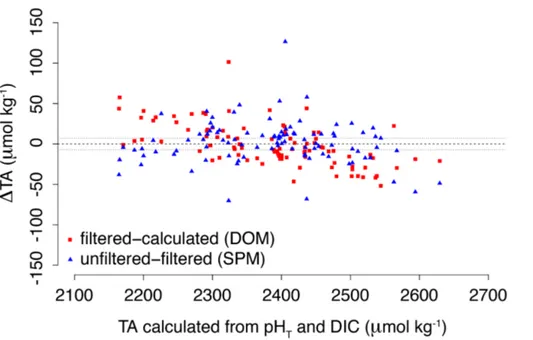
For the determination of TA, two separate samples were collected in 50 mL centrifuge tubes. To determine the contribution of suspended particulate matter to TA, one sam-ple was left unfiltered, while the other was filtered through a 0.45 µm nylon membrane

25

syringe filter (Kim et al., 2006). TA was determined using the standard operating proce-dure for open cell potentiometric titration (Dickson et al., 2007; SOP 3b), using an au-tomatic titrator (Metrohm 888 Titrando), a high-accuracy burette (1±0.001 mL), a

(9)

BGD

11, 15827–15887, 2014

coastal basin

M. Hagens et al.

Title Page

Tables Figures

◭ ◮

Back Close

Full Screen / Esc

Discussion

P

a

per

|

Discussion

P

a

per

|

Discussion

P

a

per

|

Discussion

P

a

per

|

mostated reaction vessel (T =25◦_{C) and combination pH glass electrode (Metrohm}

6.0259.100). TA values were calculated by a non-linear least-squares fit to the titration data in a custom-made script in R. Quality assurance involved regular analysis of Certi-fied Reference Materials (CRM) obtained from the Scripps Institution of Oceanography (A.G. Dickson, batches 116 and 122). The relative SD of the procedure was less than

5

0.2 % or 5 µmol kg−1(n=10).

Samples for DIC analysis were collected in 10 mL headspace vials, left to overflow and poisoned with 10 µL of a saturated mercuric chloride (HgCl2) solution. DIC

anal-ysis was performed using an AS-C3 analyser (Apollo SciTech) which consists of an acidification unit in combination with a LICOR LI-7000 CO₂/H₂O Gas Analyser.

Qual-10

ity assurance involved carrying out three replicate measurements of each sample and regular analysis of CRM. The accuracy and precision of the system are 0.15 % or 3 µmol kg−1_.

Water forpCO2analysis was collected in 50 mL glass serum bottles from the Niskin

bottle with Tygon tubing, left to overflow, poisoned with 50 µL of saturated HgCl2 and

15

sealed with butyl stoppers and aluminium caps. Samples were analysed within 3 weeks of collection by the headspace technique (Weiss, 1981) using gas chromatography (GC) with a methaniser and flame ionisation detection (FID, SRI 8610C). The GC-FID was calibrated with pure N₂and three CO₂: N₂standards with a CO₂molar fraction of 404, 1018, 3961 ppmv (Air Liquide Belgium). Headspace equilibration was done

20

overnight in a thermostated bath, and temperature was recorded and typically within 3◦_{C of in situ temperature.}_p_CO

2data were corrected to in situ temperature. Samples

were collected in duplicate and the relative SD of duplicate analysis averaged±0.8 %

(n=90)

Samples for the determination of pH were collected in 100 mL glass bottles. pH

25

(10)

cal-BGD

11, 15827–15887, 2014

coastal basin

M. Hagens et al.

Title Page

Tables Figures

◭ ◮

Back Close

Full Screen / Esc

Discussion

P

a

per

|

Discussion

P

a

per

|

Discussion

P

a

per

|

Discussion

P

a

per

|

ibration. The temperature difference between buffers and samples never exceeded 2◦C. pH values are expressed on the total hydrogen ion scale (pHT).

2.4 Community metabolism

Net community respiration (NCP), gross primary production (GPP) and community respiration (CR) were determined using the oxygen light-dark method (Riley, 1939;

5

Gazeau et al., 2005a). Samples were drawn from the Niskin bottle into similar BOD bot-tles as described in Sect. 2.2. Botbot-tles were incubated on-deck in a water bath, keeping them at ambient surface water temperature by continuous circulation of surface water. Samples were incubated both under various light intensities and in the dark. Hard neu-tral density filters with varying degrees of shading capacity (Lee Filters) were used to

10

mimic light conditions at different depths, while sample bottles incubated in the dark were covered with aluminium foil. Incubations lasted from the time of sampling (usually mid-morning) until sunset. Oxygen concentrations were determined before and after incubation using the automated Winkler titration procedure described in Sect. 2.2.

Samples incubated in the light were used to determine NCP by calculating the diff

er-15

ence in oxygen concentrations between the start and end of the incubations, divided by the incubation time (5 to 13 h). CR was determined in a similar fashion from sam-ples incubated in the dark. GPP was subsequently calculated as NCP₊CR (all rates expressed in mmol O2m−

3

h−1). To determine the relationship between algal biomass (represented as chlaconcentration) and GPP, samples from all depths were incubated

20

in triplicate at 51.2 % of surface photosynthetically active radiation (PAR). This yielded a linear relationship between [chla] and GPP for most months (data not shown). Sam-ples from one depth (typically 3 m) were incubated at 10 different light intensities to de-termine the dependency of GPP on light availability (P/I curve). These data were nor-malised to [chla] and fitted by non-linear least squares fitting using the Eilers–Peeters

25

(11)

BGD

11, 15827–15887, 2014

coastal basin

M. Hagens et al.

Title Page

Tables Figures

◭ ◮

Back Close

Full Screen / Esc

Discussion

P

a

per

|

Discussion

P

a

per

|

Discussion

P

a

per

|

Discussion

P

a

per

|

function (Eilers and Peeters, 1988):

GPPnorm=pmax

(2+ω)(I/Iopt)

(I/Iopt)2+ω(I/Iopt)+1

(2)

Here, GPP_norm is the measured GPP normalised to [chla] (mmol O₂(µg chla)−1_h−1_),

pmaxis the maximum GPPnorm (mmol O2(µg chla)− 1

h−1),I andIoptare the measured

and optimum irradiance, respectively (both in µE m−2_s−1_{) and} _ω _{is a dimensionless}

5

indicator of the relative magnitude of photoinhibition.

Downwelling light as a function of water depth was measured using a COR LI-193SA spherical quantum sensor connected to a LI-COR LI-1000 data logger. A sep-arate LICOR LI-190 quantum sensor on the roof of the research vessel connected to this data logger was used to correct for changes in incident irradiance. Light

pen-10

etration depth (LPD; 1 % of surface irradiance) was quantified by calculating the light attenuation coefficient using the Lambert–Beer extinction model. To additionally assess water-column transparency, Secchi disc depth was measured and corrected for solar altitude (Verschuur, 1997). In contrast to the measurements of downwelling irradiance, which were only taken mid-morning, Secchi depths were also determined in the

after-15

noon. Although Secchi depths cannot directly be translated into LPD estimates, they do give an indication of the seasonal and diurnal variability in subsurface light climate. Hourly averaged measurements of incident irradiance were obtained with a LI-COR LI-190SA quantum sensor from the roof of NIOZ-Yerseke, located about 31 km from the sampling site (41.489◦_{N, 4.057}◦_{E). These measurements, together with the light}

20

attenuation coefficient, were used to calculate the irradiance in the water column at each hour over the sampling day in 10 cm intervals until the LPD. Measured [chla] was linearly interpolated between sampling depths and combined with the fittedP/I curve (Eq. 2) to calculate GPP (mmol O2m−

3

h−1) at 10 cm intervals:

GPP=[chla]pmax

(2+ω)(I/Iopt)

(I/Iopt)2+ω(I/Iopt)+1

(3)

(12)

BGD

11, 15827–15887, 2014

coastal basin

M. Hagens et al.

Title Page

Tables Figures

◭ ◮

Back Close

Full Screen / Esc

Discussion

P

a

per

|

Discussion

P

a

per

|

Discussion

P

a

per

|

Discussion

P

a

per

|

These GPP values were integrated over time to determine volumetric GPP on the day of sampling (mmol O2m−

3

d−1). A similar procedure using measured hourly incident ir-radiance was followed to calculate volumetric GPP on the days in between sampling days. Parameters of the Eilers–Peeters fit were kept constant in the monthly time inter-val around the day of sampling, while [chla] depth profiles and the light attenuation

co-5

efficient were linearly interpolated between time points. These daily GPP values were integrated over time to estimate annual GPP (mmol O₂m−3yr−1).

Rates of volumetric CR (mmol O₂m−3_h−1_{) were converted to daily values}

(mmol O2m− 3

d−1) by multiplying them by 24 h. An annual estimate for CR (mmol O2m−

3

yr−1) was calculated through linear interpolation of the daily CR values

10

obtained on each sampling day. Finally, CR and GPP were converted from O2to carbon

(C) units. For CR, a respiratory coe_fficient (RQ) of 1 was used. For GPP, the production coefficient (PQ) was based on the use of ammonium (NH+₄) or nitrate (NO−₃) during primary production. Assuming Redfield ratios, when NH+₄ is taken up, this results in an O2: C ratio of 1 : 1, hence a PQ of 1. Alternatively, when the algae use NO−3, this

15

leads to an O2: C ratio of 138 : 106 and a PQ of 1.3. Since the utilisation of NH+4 is

energetically more favourable than that of NO−

3, the former is the preferred form of

dissolved inorganic nitrogen taken up during primary production (e.g., MacIsaac and Dugdale, 1972). If [NH+₄]<0.3 µmol L−1, we supposed that GPP was solely fuelled by NO−

3 uptake, while above this threshold only NH +

4 was assumed to be taken up during

20

GPP. Although we are aware that this is a simplification of reality, as NO−₃ uptake is not completely inhibited at [NH+₄]>0.3 µmol L−1(Dortch, 1990), we have no data to further distinguish between both pathways. Concentrations of NH+₄ and NO−

3 were determined

in conjunction with concentrations of phosphate (PO3₄−), silicate (Si(OH)4) and nitrite

(NO−₂) by automated colorimetric techniques (Middelburg and Nieuwenhuize, 2000)

af-25

ter filtration through 0.2 µm filters. Water for DOC analysis was collected in 10 mL glass vials and filtered over pre-combusted Whatman GF/F filters (0.7 µm). Samples were analysed using a Formacs Skalar-04 by automated UV-wet oxidation to CO2, which

(13)

BGD

11, 15827–15887, 2014

coastal basin

M. Hagens et al.

Title Page

Tables Figures

◭ ◮

Back Close

Full Screen / Esc

Discussion

P

a

per

|

Discussion

P

a

per

|

Discussion

P

a

per

|

Discussion

P

a

per

|

concentration is subsequently measured with a non-dispersive infrared detector (Mid-delburg and Herman, 2007). Nutrient and DOC data can be found in the Supplement.

2.5 Sediment fluxes

To determine DIC and TA fluxes across the sediment–water interface, we used ship-board closed-chamber incubations. Upon sediment core retrieval, the water level was

5

adjusted to circa 18–20 cm above the sediment surface. To mimic in situ conditions, the overlying water was replaced with ambient bottom water prior to the start of the incuba-tions, using a gas-tight tube and ensuring minimal disturbance of the sediment–water interface. Immediately thereafter, the cores were sealed with gas-tight polyoxymethy-lene lids and transferred to a temperature controlled-container set at in situ

tempera-10

ture. The core lids contained two sampling ports on opposite sides and a central stirrer to ensure that the overlying water remained well mixed. Incubations were done in trip-licate and the incubation time was determined in such a way that during incubation the concentration change of DIC would remain linear. As a result, incubation times varied from 6 (at S1 during summer) to 65 h (at S3 during winter).

15

Throughout the incubation, water samples (∼7 mL) for DIC analysis were collected

from each core five times at regular time intervals in glass syringes via one of the sampling ports. Concurrently, an equal amount of ambient bottom water was added through a replacement tube attached to the other sampling port. Ca. 5 mL of the sample was transferred to a headspace vial, poisoned with 5 µL of a saturated HgCl₂solution

20

and stored submerged at 4◦_{C. These samples were analysed as described in Sect. 2.3.}

The subsampling volume of 7 mL was less than 5 % of the water mass, so no correction factor was applied to account for dilution. DIC fluxes (mmol m−2d−1) were calculated from the change in concentration, taking into account the enclosed sediment area and overlying water volume:

25

J=

_∆_C ow

∆t _V

ow

(14)

BGD

11, 15827–15887, 2014

coastal basin

M. Hagens et al.

Title Page

Tables Figures

◭ ◮

Back Close

Full Screen / Esc

Discussion

P

a

per

|

Discussion

P

a

per

|

Discussion

P

a

per

|

Discussion

P

a

per

|

Here, ∆Cow

∆t is the change in DIC in the overlying water vs. time (mmol m

−3

d−1), which was calculated from the five data points by linear regression,Vow is the volume of the

overlying water (m3) andAis the sediment surface area (m2). To determine TA fluxes, no subsampling was performed. Instead, the fluxes were calculated from the difference in TA between the beginning and end of the incubation, accounting for enclosed

sed-5

iment area and overlying water volume. TA samples were collected and analysed as described in Sect. 2.3.

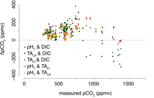
2.6 Carbonate system calculations

The measurement of four carbonate system parameters implies that we can check the internal consistency of the carbonate system (see Appendix A). For the rest of this

10

paper, we use DIC and pHTfor the carbonate system calculations. This has been

sug-gested to be the best choice when systems other than the open ocean are studied and measurements of TA may be difficult to interpret (Dickson, 2010; see also Appendix A). All calculations were performed using the R package AquaEnv. The main advantage of AquaEnv is that it has the possibility to include acid-base systems other than the

15

carbonate and borate system, which is especially important in highly productive and hypoxic waters. Furthermore, it provides a suite of output parameters necessary to compute the individual impact of a process on pH, such as the acid-base buffering ca-pacity. As equilibrium constants for the carbonate system we used those of Mehrbach et al. (1973) as refitted by Dickson and Millero (1987), which were calculated from

CTD-20

derivedT,S andpusing CO2SYS (Pierrot et al., 2006). For the other equilibrium con-stants (borate, phosphate, ammonia, silicate, nitrite, nitrate and the auto-dissociation of water) we chose the default settings of AquaEnv.

CO2air–sea exchange (mmol C m− 2

d−1) on the day of sampling was estimated using the gradient between atmosphericpCO2(pCO2, atm) and the calculated seawaterpCO2

25

at 1 m depth (both in atm):

F =kα(pCO₂−pCO2, atm) (5)

(15)

BGD

11, 15827–15887, 2014

coastal basin

M. Hagens et al.

Title Page

Tables Figures

◭ ◮

Back Close

Full Screen / Esc

Discussion

P

a

per

|

Discussion

P

a

per

|

Discussion

P

a

per

|

Discussion

P

a

per

|

Here, k (m d−1) is the gas transfer velocity, which was calculated from wind speed according to Wanninkhof (1992), normalised to a Schmidt number of 660. Daily-averaged wind speed at Wilhelminadorp (51.527◦_{N, 3.884}◦_{E, measured at 10 m}

above the surface) was obtained from the Royal Netherlands Meteorological Institute (http://www.knmi.nl). The quantityα is the solubility of CO2 in seawater (Henry’s

con-5

stant; mmol m−3_atm−1_{) and was calculated according to Weiss (1974). For} _p_CO

2, atm

we used monthly mean values measured at Mace Head (53.326◦N, 9.899◦W) as ob-tained from the National Oceanic and Atmospheric Administration Climate Monitoring and Diagnostics Laboratory air sampling network (http://www.cmdl.noaa.gov/). To cal-culate CO2 air–sea exchange on the days in between sampling days, we used

daily-10

averaged wind speed and linear interpolation of the other parameters.

2.7 Acid-base bu_ffering capacity and proton cycling

The acid-base buffering capacity plays a crucial role in the pH dynamics of natural waters. Many di_fferent formulations of this bu_ffering capacity exist (Frankignoulle, 1994; Egleston et al., 2010). However, a recent theoretical analysis (Hofmann et al., 2008)

15

has shown that, for natural waters, it is most adequately defined as the change in TA associated with a certain change in [H+], thereby keeping all other total concentrations (e.g., DIC, total borate) constant:

β=−

∂T A ∂[H+_]

(6)

Hence, when the acid-base buffering capacity of the water is high, one will observe only

20

a small change in [H+] for a given change in TA. It should be noted thatβis intrinsically different from the well-known Revelle factor (Revelle and Suess, 1957; Sundquist et al., 1979) which quantifies the CO2buffering capacity of seawater, i.e., the capacity of the

coupled ocean–atmosphere system to counteract changes in atmospheric CO2.

In this study,βwas calculated according to Hofmann et al. (2008) and subsequently

25

(16)

BGD

11, 15827–15887, 2014

coastal basin

M. Hagens et al.

Title Page

Tables Figures

◭ ◮

Back Close

Full Screen / Esc

Discussion

P

a

per

|

Discussion

P

a

per

|

Discussion

P

a

per

|

Discussion

P

a

per

|

Hofmann et al. (2010a). Briefly, each chemical reaction takes place at a certain rate and with a certain stoichiometry, e.g., aerobic respiration can be described as

CH₂O(NH₃)_γ

N(H3PO4)γP+O2→CO2+H2O+γNNH3+γPH3PO4 (R1)

whereγN andγP are the ratios of nitrogen (N) and phosphorous (P) to carbon (C) in

organic matter, respectively. At first sight, this reaction equation does not seem to

pro-5

duce any protons. However, the CO2 (as carbonic acid, H2CO3), ammonia (NH3) and

phosphoric acid (H3PO4) formed will immediately dissociate into other forms at a ratio

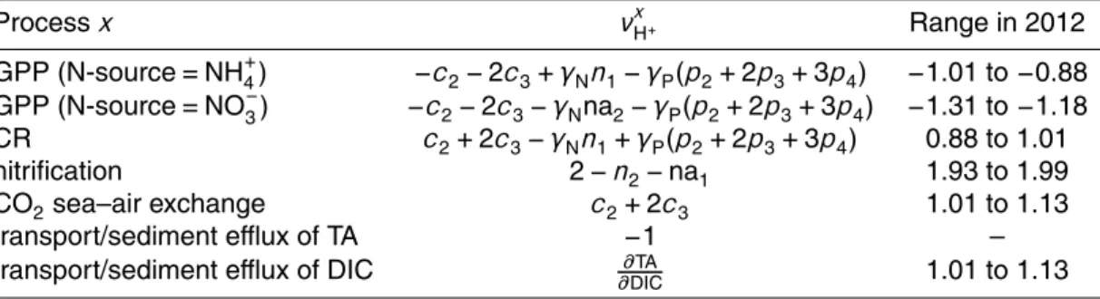
similar to their occurrence at ambient pH. As a result, protons are produced during aerobic respiration, despite the fact they are absent in Reaction (R1). The amount of protons produced is termed the stoichiometric coefficient for the proton (νx_H+) or pro-10

ton release rate. This coe_fficient is process-specific and, for aerobic respiration, equals

c2+2c3−γNn1+γP(p2+2p3+3p4) (Hofmann et al., 2010a; Table 1). Here, c2 and c3 are the ratios of bicarbonate (HCO−3) and carbonate (CO

2−

3 ) to DIC, n1 is the ratio

of NH+₄ to total ammonia, and p2,p3 and p4 are the ratios of dihydrogen phosphate

(H₂PO−

4), monohydrogen phosphate (HPO 2−

4 ) and PO 3−

4 to total phosphate,

respec-15

tively. As these ratios depend on the ambient pH, so does the value ofνx_H+.

In natural systems, the vast majority of protons produced during a biogeochemical process according toνx_H+ is consumed through immediate acid-base reactions, thereby

neutralising their acidifying effect. The extent to which this attenuation occurs is con-trolled by the acid-base buffering capacity of the system. Hence, the net change in

20

[H+] due to a certain processx (µmol kg−1d−1) is the product of the process rate (R_x; µmol kg−1d−1) and the stoichiometric coefficient for the proton of that reaction (νx_H+),

divided byβ:

d[H+]_x dt =

νx_H+

β Rx (7)

(17)

BGD

11, 15827–15887, 2014

coastal basin

M. Hagens et al.

Title Page

Tables Figures

◭ ◮

Back Close

Full Screen / Esc

Discussion

P

a

per

|

Discussion

P

a

per

|

Discussion

P

a

per

|

Discussion

P

a

per

|

The total net change in [H+] over time is simply the sum of the effects of all relevant processes, as they occur simultaneously:

d[H+]tot

dt =

1

β n X

x=1

νx_H+Rx (8)

A straightforward way to express the vulnerability of a system to changes in pH is to look at the proton turnover time (Hofmann et al., 2010a). For this we first need to define

5

the proton cycling intensity, which is the sum of all proton-producing (or consuming) processes. When dividing the ambient [H+] by the proton cycling intensity, the proton turnover time (τH+) can be estimated. The smaller the proton turnover time, the more

susceptible the system is to changes in pH. In a system that is in steady state, i.e., the final change in [H+] is zero, the proton cycling intensity is the same irrespective

10

of whether the sum of the proton producing or consuming processes is used for its calculation. In a natural system like the Den Osse Basin this is not the case, meaning that total H+ production and total H+ consumption are not equal. Here, we use the smaller of the two for the calculation of the proton cycling intensity. As a result, the calculated turnover times should be regarded as maximal values.

15

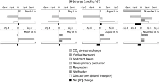
2.8 Proton budget calculations

Figure 2 shows a schematic overview of the major processes affecting proton cycling in the Den Osse Basin. For each of the four seasons (March, May, August and Novem-ber), we estimated a proton budget for the basin by calculating the net production of protons (d[H+]x

dt ) for GPP, CR, nitrification, CO2 air–sea exchange, sediment–water

ex-20

change of DIC and TA and vertical water column mixing, taking into account the effects ofS andT changes (Hofmann et al., 2008, 2009). We divided the vertical of the basin into eight depth layers, whereby the eight sampling depths represented the midpoint of each layer. Using the bathymetry of the lake, for each box we calculated the to-tal volume of water in the layer, the area at the upper and lower boundary (planar

(18)

BGD

11, 15827–15887, 2014

coastal basin

M. Hagens et al.

Title Page

Tables Figures

◭ ◮

Back Close

Full Screen / Esc

Discussion

P

a

per

|

Discussion

P

a

per

|

Discussion

P

a

per

|

Discussion

P

a

per

|

area) and the sediment area interfacing each box. The stoichiometric coefficients for the proton (νx_H+) were calculated with AquaEnv using the measured concentrations of

DIC, total phosphate, total ammonia, and total nitrate (Table 1). Rates of nitrification (mmol N m−3d−1) were estimated from the measuredT, [NH+₄] and [O₂] (in mmol m−3) using the following equation (Regnier et al., 1997):

5

Rnitr=86 400kmaxexp _T

−20

10 ln (q10)

_NH+ 4

NH+₄

+250

[O₂]

[O₂]+15 (9) Here,kmaxis the maximum nitrification rate constant (3×10−

4

mmol m−3s−1) andq10,

which is set at 2, is the factor of change in rate for a change in temperature of 10◦_C.

CO2air–sea exchange rates were converted to mmol m− 3

d−1by first multiplying them with the total surface area of the Den Osse Basin (m2) and then dividing them by

10

the volume of the uppermost box (m3), assuming that CO₂ sea–air exchange only directly affects the proton budget of this box. Similarly, DIC and TA sediment fluxes (mmol m−2d−1) were multiplied by the corresponding sediment area of the basin (m2) and then divided by the volume of the box corresponding to their measurement depth (m3). To ensure mass conservation, vertical TA and DIC transport rates (mmol d−1)

15

were computed by multiplying the difference in mass between two consecutive boxes (mmol), i.e., the product of concentration and volume, with a mixing coefficientζ (d−1) that was calculated based on the entrainment function by Pieters et al. (1985), mul-tiplied by the volume of water below the pycnocline. Then, the transport rates were converted to mmol m−3d−1 by dividing them by the volume of the corresponding box.

20

Finally, all rates (expressed in mmol m−3

d−1

) were divided by 10−3

×ρw (kg L− 1

) to convert them to µmol kg−1d−1.

The sum of d[H+]x

dt of all processes considered ( d[H+]_tot

dt ; Eq. 8) was compared with ∆[H+]_obs

∆t , which was calculated from the measured pHT as the weighted average of

the observed change in [H+] between the previous month and the current month, and

25

between the current month and the next month. The di_fference between ∆[H+]obs

∆t and

(19)

BGD

11, 15827–15887, 2014

coastal basin

M. Hagens et al.

Title Page

Tables Figures

◭ ◮

Back Close

Full Screen / Esc

Discussion

P

a

per

|

Discussion

P

a

per

|

Discussion

P

a

per

|

Discussion

P

a

per

|

d[H+]_tot

dt is represented as the closure term of the budget, which is needed because

some of the proton-producing and consuming processes are unknown or have not been measured. This budget closure term includes the effect of lateral transport induced by wind and/or water entering Lake Grevelingen through the seaward sluice, which could not be quantified due to a lack of hydrodynamic data.

5

3 Results

3.1 Environmental settings

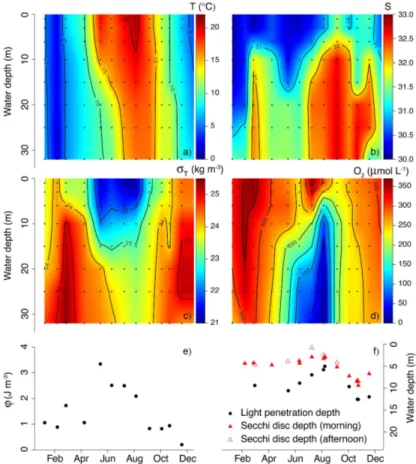
Over the year 2012, the surface water temperature at Den Osse ranged from 1.99 to 21.03◦C, while bottom water temperature showed a substantially smaller variation (1.47–16.86◦_{C; Fig. 3a). The surface water was colder than the bottom water in}

Jan-10

uary, while the reverse was true between February and April. However, the tempera-ture difference between surface and bottom water of Den Osse remained within 1◦C. Warming of the surface water in late spring rapidly increased the difference between surface and bottom water to 9.3◦C in May. This gradient persisted, albeit with decreas-ing magnitude, until August. The thermocline, which was located between 10–15 m in

15

May, deepened to 15–20 m in June. In July and August, on the contrary, temperature continuously decreased with depth. In September, the temperature depth profile was almost homogeneous, while in November and December, surface waters were again cooler than bottom waters.

Salinity (Fig. 3b) increased with water depth at all months, but the depth of the

halo-20

cline and the magnitude of the salinity gradient varied considerably over the year. This salinity gradient resulted from denser, more saline North Sea water that sank when entering Lake Grevelingen. Variations in the sluice operation, and resulting changes in North Sea exchange volumes, could therefore explain the observed month-to-month variability in salinity depth profiles. Halocline depth varied between ca. 6 m (March

25

(20)

BGD

11, 15827–15887, 2014

coastal basin

M. Hagens et al.

Title Page

Tables Figures

◭ ◮

Back Close

Full Screen / Esc

Discussion

P

a

per

|

Discussion

P

a

per

|

Discussion

P

a

per

|

Discussion

P

a

per

|

surface (30.08) and bottom (32.21) water salinity was found in March. Lower in- and outflow volumes, resulting from strict water level regulations in spring and early sum-mer (Wetsteyn, 2011), led to a lower salinity throughout the water column between April and June. In July and August, a small (∼0.2) but noticeable decrease in

salin-ity was recorded from 15–20 m onward, suggesting the intrusion of a different water

5

mass. Precipitation did not appear to exert a major control on the salinity distribution, as there was no correlation between mean water-column salinity and monthly rainfall as calculated from daily-integrated rainfall data obtained from the Royal Netherlands Meteorological Institute (http://www.knmi.nl) measured at Wilhelminadorp.

Similar to temperature, the difference in density anomaly (σ_T; Fig. 3c) between

sur-10

face and deep water was highest in May. This density gradient was sustained until August, indicating strong water-column stratification during this period. The depth of the pycnocline decreased from ca. 15 m in May and June to ca. 10 m in July and Au-gust. This corresponded to a weakening of the stratification as indicated by the strat-ification parameterφ, which dropped from 3.34 J m−3 in May to 2.09 J m−3 in August

15

(Fig. 3e). This weakening in stratification was presumably due to the delayed warming of bottom water compared to surface water. A week before sampling in September, weather conditions were stormy (maximum daily-averaged wind speed of 7.0 m s−1), which most likely disrupted stratification and led to ventilation of the bottom water. The resemblance in the spatio-temporal patterns of T,S and σT indicates that the

water-20

column stratification was controlled by both temperature and salinity, where salinity was important in winter (φvalues of ca. 1 J m−3) and temperature gradients intensified stratification in late spring and summer.

Oxygen concentrations (Fig. 3d) were highest in February as a result of the low water temperatures, increasing O2 solubility. A second peak in [O2] occurred in the

25

surface water in July, during a period of high primary production (see Sect. 3.3.1), and led to O2 oversaturation in the upper meters. From late spring onwards, water-column

stratification led to a steady decline in [O2] below the mixed-layer depth, resulting in

hy-poxic conditions (<62.5 µmol L−1) below the pycnocline in July and August. Although in

(21)

BGD

11, 15827–15887, 2014

coastal basin

M. Hagens et al.

Title Page

Tables Figures

◭ ◮

Back Close

Full Screen / Esc

Discussion

P

a

per

|

Discussion

P

a

per

|

Discussion

P

a

per

|

Discussion

P

a

per

|

August the bottom water was fully depleted of O₂, [H₂S] remained below the detection limit (5 µM), indicating the absence of euxinia. From September onwards, water-column mixing restored high O2concentrations throughout the water column.

Lake Grevelingen surface water is generally characterised by high water trans-parency and deep light penetration (Fig. 3e). LPD was 9.4 m in March and slightly

5

increased to 10.6 m in May. Between June and August, during a period of high primary production (see Sect. 3.3.1), LPD decreased until 5.8 m. From September onwards, the surface water turned more transparent again. Accordingly, LPD increased up to 12.6 m in November, after which it stabilised at a value of 12.0 m in December. The Secchi disc data generally confirm the observed temporal pattern in the LPD, as is shown by the

10

significant correlation between morning Secchi depths and LPD (r2=0.86;P <0.001). Secchi disc depth was on average∼80 % of LPD and, similar to LPD, was highest in

November and lowest in July. Additionally, the Secchi depths indicate that diurnal vari-ations in light penetration may exist. Especially in July, during an intense dinoflagellate bloom (see Sect. 3.3.1), light penetrated much deeper into the water column in the

15

morning than in the afternoon (Secchi disc depths of 2.9 and 0.9 m, respectively). The di_fference between morning and afternoon Secchi disc depth was much smaller in Au-gust (3.3 and 2.5 m) and virtually absent in November (8.5 and 8.4 m).

3.2 Carbonate system variability

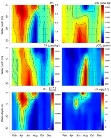
3.2.1 pHT, DIC, TA,pCO2

20

In January, pHT showed little variation with depth, with an average value of 8.04

(Fig. 4a). From February to April, pHT increased throughout the water column, though

the increase was faster at the surface than at depth, up to a maximum of 8.36 in the surface water in April. From June onward, stratification augmented the difference be-tween surface and bottom water pHT. In August, this difference had increased to 0.69

25

(22)

BGD

11, 15827–15887, 2014

coastal basin

M. Hagens et al.

Title Page

Tables Figures

◭ ◮

Back Close

Full Screen / Esc

Discussion

P

a

per

|

Discussion

P

a

per

|

Discussion

P

a

per

|

Discussion

P

a

per

|

pH and low [O₂] in seasonally stratified waters. Additionally, elevated surface water pHT in summer co-occurred with high [O2], concurrent with an intense dinoflagellate

bloom (see Sect. 3.3.1). Similar to the depth profiles of [O2], the termination of

stratifi-cation diminished the gradient between surface and bottom-water pH_T. However, pH_T at the end of 2012 was significantly lower (average value of 7.98) than at the beginning

5

of 2012. Over the year, surface-water pHT varied 0.46 units, while bottom-water pHT

variation was higher (0.60 units).

DIC (Fig. 4b) showed little variation with depth in January and February (average value 2257 µmol kg−1), with the exception of the bottom water, where DIC was slightly (40–50 µmol kg−1) elevated. In March, DIC decreased slightly throughout the water

col-10

umn, with a stronger drawdown in the upper 6–10 m, and the higher bottom-water concentrations diminished. The gradient between surface and deeper water intensi-fied until ca. 70 µmol kg−1 in April, due to an increase in bottom-water DIC. In May, a concurrent drawdown in DIC above 15 m and increase in DIC below this depth re-sulted in a surface-to-bottom DIC gradient of 250 µmol kg−1. The depth of this sharp

15

gradient coincided with the pycnocline depth. In June, DIC increased strongly (by 100–200 µmol kg−1

) below the pycnocline, while in July and August, a strong draw-down in DIC occurred above the pycnocline, concurrent with an intense dinoflagellate bloom (see Sect. 3.3.1). In combination with the persisting stratification, this resulted in a DIC gradient of 600 µmol kg−1_{. After the disruption of the stratification, the gradient}

20

between surface and bottom water DIC was strongly reduced, and decreased further from 144 to 47 µmol kg−1 between September and December. Concomitantly, the av-erage DIC increased from 2146 to 2201 µmol kg−1_{, although the month October was}

characterised by overall slightly lower DIC (average value of 2123 µmol kg−1). Surface-water DIC variation over the year (453 µmol kg−1) was somewhat higher than in the

25

bottom water (361 µmol kg−1_).

TA (Fig. 4c) generally showed more temporal than spatial variability. Therefore, vari-ations in TA with depth were usually much smaller compared to DIC. In January and February, TA was fairly constant with depth (average value of 2404 µmol kg−1_{), with the}

(23)

BGD

11, 15827–15887, 2014

coastal basin

M. Hagens et al.

Title Page

Tables Figures

◭ ◮

Back Close

Full Screen / Esc

Discussion

P

a

per

|

Discussion

P

a

per

|

Discussion

P

a

per

|

Discussion

P

a

per

|

exception of bottom-water TA in January (2460 µmol kg−1). In March and April, TA in the upper 6 m was 40–50 µmol kg−1 higher than in the underlying water. Overall, TA in April had increased by on average 105 µmol kg−1

compared to March. The period of water-column stratification was characterised by a positive surface-to-bottom-water TA gradient correlating with pycnocline depth. This gradient was strongest in June

5

(195 µmol kg−1_{), as a result of high bottom-water TA, and in August (306 µmol kg}−1_),

mainly due to the strong drawdown in surface-water TA. Because of this, average water-column TA in June was much higher (2520 µmol kg−1) than in August (2366 µmol kg−1). The low surface-water TA persisted until November, while TA below 10 m depth was much less variable. Similar to DIC, the month October was characterised by overall

10

lower TA. There was little difference between surface and bottom-water variation in TA over the entire year (372 and 337 µmol kg−1_{, respectively).}

The pattern ofpCO2(Fig. 4d) was inversely proportional to that of pHT. January was

characterised by little variation with depth and an averagepCO2 (404 ppmv) close to pCO_{2, atm} (396 ppmv). In February, lowT throughout the water column led to a

draw-15

down ofpCO2 which continued until April, albeit with larger magnitude in the surface

compared to the bottom water. The onset of stratification in May led to a build-up of CO2

resulting from organic matter degradation in the bottom water. Maximum bottom-water

pCO2(1399 ppmv) was found in August and, as expected, co-occurred with the period

of most intense hypoxia (Fig. 3d). While in May and June,pCO2increased throughout

20

the water column, in July and August, a substantial drawdown in surface-waterpCO₂ was observed coinciding with an increase in [O2], which is indicative of high autotrophic

activity. Water-column ventilation disrupted the surface-to-bottompCO2 gradient from

September onwards. Mean water-columnpCO₂ decreased from 584 to 490 ppmv be-tween September and December, althoughpCO2values were slightly higher in

Novem-25

ber, especially in the bottom water (601 ppmv on average). Note that, in contrast to Jan-uary, the average water-columnpCO₂ in December was much higher than pCO_{2, atm} (398 ppmv). Similar to pHT, pCO2 variation over the year was higher in the bottom

(24)

BGD

11, 15827–15887, 2014

coastal basin

M. Hagens et al.

Title Page

Tables Figures

◭ ◮

Back Close

Full Screen / Esc

Discussion

P

a

per

|

Discussion

P

a

per

|

Discussion

P

a

per

|

Discussion

P

a

per

|

We investigated the correlation between the different carbonate system parameters and O2by calculating coefficients of determination and testing their significance using

the package Stats in R. In line with our visual observations, we found a strong correla-tion between pH_T andpCO₂(r2=0.89,P <0.001) and weak to moderate correlations between pH_Tand O₂(r2=0.68,P <0.001),pCO₂and O₂(r2=0.70,P <0.001), and

5

DIC and TA (r2=0.56, P <0.001). DIC does not appear to be correlated with pHT

(r2=0.18, P <0.001), pCO2 (r 2

=0.17, P <0.001) or O2 (r 2

=0.21, P <0.001). Fi-nally, TA could not statistically significant be correlated to pHT (r

2

=0.01, P =0.278),

pCO₂(r2=0.01,P =0.384) or O₂(r2=0.04,P =0.066).

3.2.2 Acid-base buffering capacity 10

The acid-base buffering capacity generally showed a similar spatio-temporal pattern as pHT and the inverse of thepCO2pattern (Fig. 4e). In January,βhad an average value

of 22 967 and hardly varied with depth. From February to April, the buffering capacity increased throughout the water column, with a faster increase in the surface compared to the bottom water and a maximum of 82 557 in the surface water in April. In May

15

and June, the acid-base buffering capacity showed an overall decline. In contrast to pH_T, the onset of stratification did not lead to a direct amplification of the di_fference between surface and bottom waterβ. July was characterised by a sharp increase in surface-waterβ, coinciding with the decrease in DIC, and a decrease in bottom-water

β, a trend that was further intensified in August. During this period of strongest

hy-20

poxia, surface-waterβ (71 454) was an order of magnitude higher than bottom-water

β(6802). Between September and December, i.e., after bottom-water ventilation, the bu_ffering capacity did not show any substantial variations with depth. Over the course of the year, surface-waterβvaried a factor 2 more than bottom-waterβ.

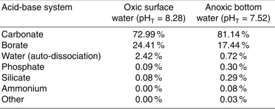
To further elucidate what controls the acid-base buffering capacity, we calculated

25

the contribution of various acid-base systems toβfor the surface and bottom water in August (Table 2). This calculation shows that in the oxic surface water, whereβis high,

(25)

BGD

11, 15827–15887, 2014

coastal basin

M. Hagens et al.

Title Page

Tables Figures

◭ ◮

Back Close

Full Screen / Esc

Discussion

P

a

per

|

Discussion

P

a

per

|

Discussion

P

a

per

|

Discussion

P

a

per

|

the relative contribution of the borate system to the total buffering capacity was higher than in the anoxic, poorly-buffered bottom water (24 and 17 %, respectively), while the reverse holds for the carbonate system (73 vs. 81 %). Acid-base systems other than the carbonate and borate system contributed most to the buffering capacity in the anoxic bottom water, due to the accumulation of NH+₄, PO3₄− and Si(OH)4. However, their total

5

contribution never exceeded 1 %.

3.3 Rate calculations

3.3.1 Gross primary production and community respiration

chla, which was used as an indicator for algal biomass, showed three periods of ele-vated concentrations (Fig. 4f). In March, surface-water [chla] showed a slight increase

10

up to 5.2 µg L−1. In May, elevated [chla] could be found between 6–15 m, with a subsur-face maximum of 19.0 µg L−1at 10 m depth. Finally, the most prominent peak in [chla] (27.3 µg L−1) was found in the surface water in July. Together with elevated [O₂] and pHT and a drawdown of DIC andpCO2, this indicated the presence of a major

phyto-plankton bloom. Microscopic observations of phytophyto-plankton samples from this bloom

15

showed it consisted mainly of the dinoflagellateProrocentrum micans.

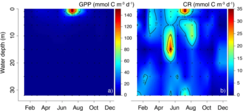
Measured volumetric rates of GPP ranged from 0.0–150.7 mmol C m−3d−1(Fig. 5a), while volumetric CR ranged from 0.0–31.5 mmol C m−3d−1(Fig. 5b). To a large extent, their spatio-temporal patterns confirm the trends in [chla]. GPP showed a distinct sea-sonal pattern, with one major peak in July 2012 (151 mmol C m−3d−1 at 1 m depth)

20

coinciding with high surface water [chla] and CR (31 mmol C m−3d−1). Elevated CR in August between 6–10 m depth (19 mmol C m−3d−1) may reflect degrading algal mate-rial from this bloom. Although surface water [chla] showed a slight increase in March, this was not reflected in the GPP during this month (maximum 9.4 mmol C m−3d−1). The peak in [chla] in May correlated with a major peak in CR (maximum 31 mmol C m−3d−1)

25