doi: 10.5540/tema.2018.019.02.0209
Numerical Solution of Heat Equation with
Singular Robin Boundary Condition
†G. LOZADA-CRUZ1, C.E. RUBIO-MERCEDES2and J. RODRIGUES-RIBEIRO3
Received on April 17, 2017 / Accepted on November 23, 2017
ABSTRACT. In this work we study the numerical solution of one-dimensional heat diffusion equation subject to Robin boundary conditions multiplied with a small parameter epsilon greater than zero. The numerical evidences tell us that the numerical solution of the differential equation with Robin boundary condition are very close in certain sense of the analytic solution of the problem with homogeneous Dirichlet boundary conditions whenεtends to zero.
Keywords: Eigenvalue Problems, Finite Difference Method, Robin Boundary Conditions, Numerical Solutions.
1 INTRODUCTION
It is well known that the diffusion differential equation models the transient conduction phe-nomenon that occurs in numerous engineering applications and may be analyzed by using dif-ferent analytic and numerical methods. Many transient problems involving geometry and sim-ple boundary value conditions, their analytic solution are known explicitly, especially the one-dimensional (1D) case. Still for the two-one-dimensional (2D) and three-one-dimensional (3D) cases some of the analytic solutions are known (see [1, 2]). However, in most cases, the geometry or boundary conditions make it impossible to apply analytic techniques to solve the heat diffusion equation.
†Work presented at the XXXVI National Congress of Applied and Computational Mathematics, Gramado, RS, Brazil,
2016.
*Corresponding author: Cosme Eustaquio Rubio Mercedes – E-mail: [email protected]
1Departamento de Matem´atica, Instituto de Biociˆencias, Letras e Ciˆencias Exatas, Universidade Estadual Paulista (Unesp), 15054-000, S˜ao Jos´e do Rio Preto, SP, Brazil. E-mail: [email protected]
2Programa de Matem´atica e Engenharia F¨ısica, Universidade Estadual do Mato Grosso do Sul (UEMS), Dourados, MS, Brazil. E-mail: [email protected]
In this work we use the Crank-Nicolson Finite Difference Method (FDM) (see [9]) to solve the 1D heat diffusion equation in transient regime with Robin boundary conditions given by
ut=uxx,−1<x<1,t>0,
−εux(−1) =u(−1), εux(1) =u(1),
(1.1)
whereε∈(0,1].
Ifε=0 in (1.1) we have the classical problem with homogeneous Dirichlet boundary conditions for the heat equation which is well known.
There is great interest on heat problems and much work was done considering different bound-ary conditions. Nevertheless, the particular (1.1) problem with singular boundbound-ary conditions, depending on a positive parameter, has not been studied previously neither analytically nor nu-merically. Our little contribution with this kind of problems which depend of a small parameter is to show numerical solutions when we vary the values ofε.
Many problems in the industry are modeled by the heat equation subject to specific initial and boundary conditions, and sometimes it is not possible to get the analytic solution. Actually many researchers use different numerical techniques to understand the behavior of the solution (for more details see [5, 6, 10] and in references therein).
This paper is organized as follows. In Section 2, we state that the equation (1.1) has unique solution for eachε>0. Also we study asymptotic behaviour of the eigenvalues of (Eε) whenε tends to zero. In Section 3 a brief description of the problem with Robin boundary condition in conjunction with the FDM approach is presented. The numerical experiments are discussed in Section 4, and finally the conclusions are presented in Section 5.
2 ON THE EXISTENCE OF SOLUTION
LetΩ= (−1,1)and the Lebesgue spaceX=L2(Ω). LetAε :D(Aε)⊂L2(Ω)→L2(Ω)be an
unbounded linear operator defined through
D(Aε) =u∈H2(Ω):−εux(−1) =u(−1),εux(1) =u(1) , (2.1)
Aεu=u′′. (2.2)
Thus we can write the equation (1.1) as an evolution equation inL2(Ω)(see [7]) as follows
( ˙
u=Aεu,t>0,
u(0) =u0∈H1(Ω).
(2.3)
Theorem 1.For each u0∈H1(Ω), there exists a unique solution u=u(t,u0)of (2.3) defined on
its maximal interval of existence[0,τu0)which mean that eitherτu0 = +∞, or ifτu0 <∞them
lim sup t→τu−0
Proof.See [1, 7].
It is well known that for a fixed valueε>0, the problem (2.3) generates a well-defined linear semigroup inH1(Ω), the solutions enterW1,p(Ω)for anypsuch that 1<p<∞and are classical fortpositive (for more details see [1, 7]).
2.1 Equilibrium solution for (1.1)
The equilibrium solution of (1.1) satisfy the elliptic boundary value problem
uxx=0,t>0,−1<x<1,
−εux(−1) =u(−1),
εux(1) =u(1).
(2.4)
Theorem 2.For everyε>0the unique equilibrium solution of (2.4) is uε≡0.
Proof.The solution of the problem (2.4) is given by
u(x) =u(1)−u(−1) 2
x+u(1) +u(−1)
2 , x∈Ω. (2.5)
By the boundary conditions (2.4) in (2.5) we have thatu(−1)andu(1)satisfy
u(1) =εu(1)−u(−1)
2 =−u(−1). (2.6)
Thus we haveu(−1) +u(1) =0, and (2.5) provides
u(x) =u(1)−u(−1) 2
x. (2.7)
Again, by using the boundary conditions (2.4) we have
u(1)−u(−1)
2 =ε
u(1)−u(−1)
2 , (2.8)
and forε6=1 we have
u(1)−u(−1) =0. (2.9)
Finally, from (2.9) we conclude thatuε≡0.
Remark 3.From the Theorem 2 we can say that uε≡0converges to the solution u≡0of the
2.2 Eigenvalue problem
Consider the eigenvalue problem associated with the linear operatorAε
uxx=λεu, inΩ,
−εux(−1) =u(−1),
εux(1) =u(1).
(Eε)
For eachε>0, the problem (Eε) has a sequence of real eigenvalues{λε
n}∞n=1, with anL2(Ω)
-orthogonal and complete associated system of eigenfunctions {ϕε
n}∞n=1. This conclusion is
possible because the operatorAεis densely defined closed and self-adjoint inL2(Ω).
From (2.4) we conclude that zero is not an eigenvalue for (Eε). The variational formulation for λnεis given by
λnε=ψmin∈ Yn
ε(ψ′(1)2+ψ′(−1)2)−R
Ω|ψ′|2
R Ω ψ2 , (2.10) where
Yn= n
w∈C2(Ω):w6=0,w
1
−1=±εw
1
−1, Z
Ω
wϕεj =0,∀j=1,2,· · ·,n−1 o
.
For more details about the variational formulation of boundary value problems see for example [3, Chapter 8] and [4, Chapter 5].
Letλε =ω2,ω ∈R, and ϕε(x)=cosh(ωx)the eigenfunction associated with λε. From the
boundary conditions forϕε, we have
tanhω= 1
εω. (2.11)
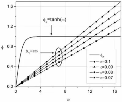
The solutions of (2.11) can be determined numerically. They can also be obtained approximately by sketching the graphs ofψ1(ω) =tanhω andψ2(ω) = εω1 forε=0.1,0.09,0.08,0.07, and
identifying the points of intersection of the curves (see in Fig. 1). Letω1(ε)be the interception
points of the curvesψ1(ω)andψ2(ω). Thusλ1ε=ω1(ε)2.
Now, taking the eigenfunctionϕε(x) =sinh(ωx)and using the boundary condition, we have
tanhω=εω. (2.12)
In Fig. 2 we also have plotted the graphs of φ1(ω) =tanhω and φ2(ω) = εω for ε =
0.1,0.09,0.08,0.07, as function ofω. Letω2(ε)be the interception points of the curvesφ1(ω)
andφ2(ω). Thusλ2ε=ω2(ε)2.
From Figs. 1 and 2 we can observe that the eigenvaluesλε
1 andλ2ε increase continually whenε
Figure 1: Graphical solution of tanh(ω) =εω1 forε=0.1,0.09,0.08,0.07.
Lemma 4.Letε>0. Thenλ1ε>λ2ε. Moreoverλ1ε,λ2ε→∞whenε→0.
Proof.We know that the functions tanhωand cothωcan be write as
tanhω = 1−2e−2ω+2e−4ω−2e−6ω+· · · (2.13)
cothω = 1+2e−2ω+2e−4ω+2e−6ω+· · · (2.14)
From the equation (2.11), we have
ω=1 ε
1
tanhω. (2.15)
Whenωis large enough, tanhω approaches 1. Thus, from (2.15) we have
ω=1 εcoth 1 ε = 1 ε
1+2e−2/ε+2e−4/ε+2e−6/ε+· · ·. (2.16)
Sinceλε
1 =ω1(ε)2, we have
λ1ε= 1 ε2+
4 ε2e
−2/ε+ 8
ε2e
−4/ε+· · ·. (2.17)
From (2.12) we obtain
ω=1
εtanhω. (2.18)
Whenωis large enough, tanhω approaches 1. Thus, from (2.18) we have
ω=1 εtanh 1 ε = 1 ε
1−2e−2/ε+2e−4/ε−2e−6/ε+· · ·. (2.19)
Sinceλε
2 =ω2(ε)2, we have
λ2ε=
1 ε2−
4 ε2e
−2/ε+ 8
ε2e
−4/ε− · · ·. (2.20)
From (2.17) and (2.20) follow the results.
Also from (2.17) and (2.20) we have that the gap betweenλε
1 andλ2εis given by
λ1ε−λ2ε≈ 8
ε2e
−2/ε. (2.21)
Remark 5.Whenεtends to zero, the problem (Eε) becomes
(
uxx=λ0u, −1<x<1,
u(−1) =u(1) =0. (
E0)
We known that the eigenvalues of the problem (E0) are given byλ0
n =−n2π2, n∈N.
Whenεtends to infinity, the problem (Eε) becomes
(
uxx=λ0u, −1<x<1,
ux(−1) =ux(1) =0.
3 THE FDM APPROACH
In this section we present the numerical schemes to solve (1.1) by applying the finite difference method (FDM) combined with the classic and unconditionally stable Crank-Nicolson method (see [8]).
To solve (1.1), the spatial domain[−1,1]is discretized with uniform grid ofndivisions of sizeh, where each spatial nodal points arexi=ih−1. Similarly, the temporal domain[0,T]is divided inmparts of sizek, whereT>0 and the temporal nodal points are indexed bytj=jk. With this indexes, we can use the following notation for the values ofu:ui j=u(xi,tj)andui=u(xi,t).
From the boundary condition given in (1.1) atx=−1 and forε>0 we write
ux(−1,t) =
−u(−1,t) ε .
Assuming that atx=−1, the functionuis twice differentiable inx, so that we can write
uxx(−1,t) =
−ux(−1,t)
ε =
u(−1,t) ε2 ,
and in the same way atx=1 we get
uxx(1,t) =
ux(1,t)
ε =
u(1,t) ε2 .
Also, by using the finite difference approach foruxx(t)(see [9]), the problema (1.1) can be write
dui(t)
dt =
ui+1(t)−2ui(t) +ui−1(t)
h2 (3.1)
fori=1, ...,n−1, and fori=0 andi=n, we have
du0(t)
dt = u0(t)
ε2 , (3.2)
and
dun(t)
dt = un(t)
ε2 , (3.3)
respectively. Thus by using (3.1)-(3.3), the problem (1.1) can be transformed into the first-order matrix differential equation given by
∂ ∂t u0 u1 u2 .. .
un−2
un−1
un = 1 h2 h2
ε2 0 0 · · · 0 0 0
1 −2 1 . .. 0
0 1 −2 . .. ... 0
..
. . .. ... ... ... ... ...
0 . .. ... −2 1 0
0 . .. 1 −2 1
0 0 0 · · · 0 0 hε22
u0 u1 u2 .. .
un−2
un−1
or in compact way
dU
dt =LU, (3.5)
where, the matrixLrepresents the discrete counterpart of the corresponding differential operator given in (1.1), which is a tridiagonal band matrix andUdenotes a vector with the unknown values ofudefined over the nodes of the spatial mesh.
There are two general methods to solve (3.5): the explicit and implicit finite difference schemes. The type of implicit scheme adopted in this work was the Crank-Nicolson algorithm (see [8]).
4 NUMERICAL RESULTS
For the numerical examples we consider the initial condition given by
u(x,0) =cosπ 2x
, (4.1)
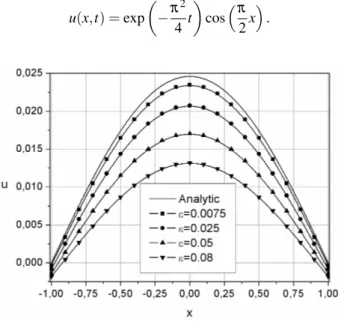
where for homogeneous Dirichlet boundary condition, which is obtained from (1.1) withε=0, the analytical solution is
u(x,t) =exp
−π
2
4 t
cosπ 2x
. (4.2)
Figure 3: Numerical solutions of (1.1) whenε→0 att=1.5.
Figure 4: Numerical solutions of (1.1) whenε→0 atx=0.8.
Table 1: Absolute errorkua−unkin function ofx calculated from the data of Fig. 3.
0.0075 0.025 0.05 0.08
0 0.0012 0.0040 0.0076 0.0115 0.1000 0.0012 0.0039 0.0076 0.0114 0.2000 0.0012 0.0038 0.0076 0.0111 0.3000 0.0011 0.0036 0.0070 0.0105 0.4000 0.0010 0.0034 0.0065 0.0098 0.5000 0.0010 0.0031 0.0059 0.0088 0.6000 0.0009 0.0027 0.0052 0.0077 0.7000 0.0007 0.0023 0.0044 0.0064 0.8000 0.0006 0.0019 0.0034 0.0050 0.9000 0.0005 0.0014 0.0025 0.0034 1.0000 0.0003 0.0008 0.0014 0.0018
in Tables 1 and 2, we can see that the numerical solutions of (1.1), which is a boundary value problem with Robin boundary conditions, converges to the exact solution of the problem with homogeneous Dirichlet boundary conditions, whenεtends to zero.
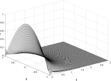
Figure 5: Temporal evolution of the numerical solution obtained with initial condition given by (4.1) and forε=0.05.
Table 2: Maximum error norm of the difference of solutionsuaandun.
Simulation ε kua−unk
1 0.0075 0.00121
2 0.0250 0.00395
3 0.0500 0.00765
4 0.0800 0.01151
5 CONCLUSIONS
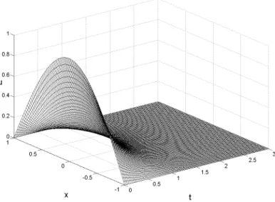
Figure 6: Temporal evolution of the analytical solution obtained in (4.2), with initial condition given by (4.1).
ACKNOWLEDGEMENTS
G. Lozada-Cruz is partially supported by the S˜ao Paulo Research Foundation (FAPESP, grant: 2015/24095-6). C.E. Rubio-Mercedes is supported by The Mato Grosso do Sul Research Founda-tion (FUNDECT, grant: 219/2016). J. Rodrigues-Ribeiro is partially supported by CoordinaFounda-tion for the Improvement of Higher Education Personnel (CAPES, grant: PICME-9725290/M).
The authors are grateful to the referee for valuable remarks improving the original version of the paper.
RESUMO. Neste trabalho, obtemos soluc¸˜oes num´ericas da equac¸˜ao diferencial de difus˜ao do calor unidimensional com um parˆametro pequenoεnas condic¸˜oes de contorno de Robin. Exemplos num´ericos demonstram que as soluc¸˜oes num´ericas do problema com condic¸˜ao de contorno de Robin convergem para a soluc¸˜oes anal´ıticas do problema de Dirichlet homogˆeneo quandoεtende a zero.
Palavras-chave: Problema de Autovalores, M´etodo de Diferenc¸as Finitas, Condic¸˜oes de Contorno de Robin, Soluc¸˜oes Num´ericas.
REFERENCES
[2] T.L. Bergman, A.S. Lavine, I.F. P. & D.P. Dewitt. “Fundamentals of Heat and Mass Transfer”. 7th ed., John Wiley and Sons, Inc. (2007).
[3] H. Brezis. “Functional analysis, Sobolev spaces and partial differential equations”. Springer, New York (2011).
[4] G. Buttazzo, M. Giaquinta & S. Hildebrandt. “One-dimensional variational problems. An introduction”, volume 15. The Clarendon Press, Oxford University Press, New York (1998).
[5] L.D. Chiwiacowsky & H. de Campos Velho. Different Approaches for the Solution of a Backward Heat Conduction Problem.Inverse Problems in Engineering, (3) (2010), 471–494.
[6] R. Das, S. Mishra, T. Kumar & R. Uppaluri. An Inverse Analysis for Parameter Estimation Applied to a Non-Fourier Conduction-Radiation Problem.Heat Transfer Engineering,32(6) (2011), 455–466.
[7] D. Henry. “Geometric theory of semilinear parabolic equations”, volume 840. Springer-Verlag, Berlim (1981).
[8] H.E. Hern´andez-Figueroa & C.E. Rubio-Mercedes. Transparent boundary for the finite element simulation of temporal soliton propagation.IEEE Transaction on Magnetics,34(5) (1998).
[9] J.D. Hoffman. “Numerical Methods for Engineers and Scientists”. Marcel Dekker, Inc., New York, 2nd edition (2001).