FUNDAÇÃO GETULIO VARGAS
ESCOLA DE ADMINISTRAÇÃO DE EMPRESAS DE SÃO PAULO
MAXENCE CARL FRANÇOIS SCICHILI
LIQUIDITY PROXIES IN THE BRAZILIAN DEBENTURE MARKET
FUNDAÇÃO GETULIO VARGAS
ESCOLA DE ADMINISTRAÇÃO DE EMPRESAS DE SÃO PAULO
MAXENCE CARL FRANÇOIS SCICHILI
LIQUIDITY PROXIES IN THE BRAZILIAN DEBENTURE MARKET
Thesis
presented
to
Escola
de
Administração de Empresas de São
Paulo of Fundação Getulio Vargas, as a
requirement to obtain the title of Master
in International Management (MPGI).
Knowledge Field: Gestão e
Competitividade em Empresas Globais
Adviser: Prof. Dr. Lauro Gonzalez
Farias
Scichili Maxence
Liquidity proxies in the Brazilian debenture market / Maxence Scichili– 2015
47f.
Orientador: Gonzalez Farias, Lauro
Dissertação (MPGI) - Escola de Administração de Empresas de São Paulo.
1. Debêntures - Brasil. 2. Mercado de capitais - Brasil. 3. Liquidez (Economia)I.
Lauro, Gonzalez Farias. II. Dissertação (MPGI) - Escola de Administração de
Empresas de São Paulo. III. Liquidity Proxies in the Brazilian Debenture Market
MAXENCE CARL FRANÇOIS SCICHILI
LIQUIDITY PROXIES IN THE BRAZILIAN DEBENTURE MARKET
Thesis
presented
to
Escola
de
Administração de Empresas de São
Paulo of Fundação Getulio Vargas, as a
requirement to obtain the title of Master
in International Management (MPGI).
Knowledge Field: Gestão e
Competitividade em Empresas Globais
Approval Date
____/____/_____
Committee members:
_______________________________
Prof. Dr. Lauro Gonzalez Farias
_______________________________
Prof. Dr. Marcio Gabrielli
ABSTRACT
This study analyzes liquidity proxies in the Brazilian debenture corporate market and tests the Eurobond proxy to better understand which characteristics help predict the liquidity of debentures.
Although Brazilian capital markets have improved drastically over the past years, big Brazilian corporations have many options when deciding to raise capital (the issuance of Eurobond is one of them). This study seeks to fill a gap in the academic literature by seeing if a liquidity relationship exists between the 2 markets.
The Eurobond proxy was found to be significant at the 5% level and 1% level.
The other proxies that were found to be significant (Issue Amount, Initial Maturity, Rating) match the results of previous studies from our literature review.
KEY WORDS:
BRAZILIAN CAPITAL MARKETS, LIQUIDITY PROXIES,
RESUMO
Este estudo analisa as variáveis de liquidez no mercado corporativo brasileiro de debêntures e testa a variável Eurobond para compreender quais características ajudam a prever a liquidez de debêntures.
Embora os mercados de capitais brasileiros tenham melhorado drasticamente nos últimos anos, as grandes empresas brasileiras têm muitas opções na hora de tomar a decisão de aumentar capital (emissão de Eurobônus é um deles). Este estudo busca preencher uma lacuna na literatura acadêmica vendo se existe uma relação de liquidez entre os dois mercados.
O proxy Eurobond foi encontrado significativo ao nível de 5% e o nível de 1%. Os outras proxies que foram significativos (valor de emissão, data de vencimento inicial, Avaliação) coincidem com os resultados de estudos anteriores.
PALAVRAS CHAVE: MERCADO DE CAPITAL, PROXIES DE LIQUIDEZ,
SUMMARY TABLE
1 INTRODUCTION 9
2 LITTERATURE REVIEW 12
2.1 Definition of liquidities, proxies and modeling 12
2.2 Brazilian Bonds 14
2.3 Offshore Bonds 17
3 METHODOLOGY 20
3.1 Description of the variables 20
3.2 Dependent variables 20
3.2.1 Volume traded (AV) 20
3.2.2 Number of transactions (NT) 21
3.3 Independent variables 21
3.3.1 Rating (Rcp) 22
3.3.2 Size of the issue (size) 23
3.3.3 Initial Maturity of Security 23
3.3.4 Type of issuers 23
3.3.5 Eurobonds 24
3.4 Selection of the samples 24
3.5 Selection of the characteristics of our debentures 26
3.5.1 Correlation 26
3.5.2 Regression analysis 26
4 ANALYSIS 28
4.1 Descriptive analysis of samples 28
4.1.1 Descriptive analysis of Debenture sample 1 28
4.1.2 Descriptive analysis of Debenture sample 2 31
4.2 Regression analysis 33
4.2.1 Regression of Debenture sample 1 33
4.2.2 Regression of Debenture sample 2 33
4.3 Analysis of Results 38
4.3.1 Results from the regression analysis 40
6 REFERENCES 43
7 APPENDIXES 46
7.1 Appendix 1: Sample 1 Debenture 46
1 INTRODUCTION
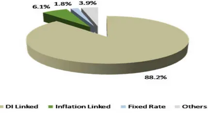
Corporate debenture market in Brazil is one of the most active markets in Latin America. According to Dealogic in 2013, Brazil ranked amongst the top LATAM countries in terms of corporate bond issuances with corporate bond activity reaching 1.71% of GDP. The Brazilian debt capital market displays unique characteristics such as high interest rates, overwhelming government bonds, high percentage of short to medium term maturity indexed or inflated adjusted security and low liquidity which differentiates it from other mature market.
The growth of this market has enabled to attend the growing credit demand from corporations (The volume of total debentures issued has gone from R$ 6.3 bn in 2008 to R$ 48.5 bn in 2011 according to Anbima). Regulatory changes orchestrated by the CVM such as instruction 476 have facilitated the issuance process which has resulted in a sharp increase in the local debt capital market primary market.
In parallel, issuance of Brazilian US$ denominated bonds have also grown at fast pace during the 2008-2014 period and the majority of the issuances have been from Corporate and Financial institution (graph 2). Foreign debt compared to Brazilian debt has generally longer terms which is one of the advantage for corporations. Although both capital markets can be seen as
complimentary in the case of a Eurobond issued by a Brazilian company to fund a project abroad in US$; a Eurobond can also be a substitute to a debenture using a currency swap. Black and Munro (2010) have identified such reasons amongst the corporate issuers in the Asia Pacific region
Graph 1 LATAM USD Denominated Bond Issuances (volume in USD bn)1
Source: Anbima
Graph 2 Brazil USD Denominated Bond Issuances (volume in USD bn)1
Source: Anbima
This study seeks to analyze liquidity proxies in the Brazilian debenture corporate market and test the Eurobond proxy to better understand which characteristics help predict the liquidity of debentures. Although Brazilian capital markets have improved drastically over the past years, big Brazilian corporations have many options when deciding to raise capital (the issuance of Eurobond is one of them). This study seeks to fill a gap in the academic literature by seeing if a liquidity relationship exists between the 2 markets.
Liquidity as defined by Amihud and Mendelson (1991) is often seen as the ability to buy or sell a security relatively fast without affecting the price of that security. Due to the nature of the over the counter market with no centralized operations and little trading activity in which corporate bonds are exchanged, academics as well as investment banks have had to look for indirect measures.
Latam USD Bond Issuances
In order to understand the proxies that best measure liquidity in the Brazilian debenture market we will ask ourselves the following question:
1) Does issuing a Eurobond for a Brazilian company increase the liquidity of its debenture?
First, we define proxies as indicators that estimate a phenomenon because of the lack of direct signs. The proxies that we will use to test for liquidity are rating, size of the issue, initial maturity, type of issuers and Eurobonds. Secondly, we define liquidity as an indicator of the depth, tightness and resilience of a market (Amante & Araujo, 2007). Depth measures the capability of a market to take in large transactions without a significant price movement, tightness measures the cost efficiency of transactions and resilience indicates the capability for the market to absorb shock.
2 LITTERATURE REVIEW
Extensive research has been done on the liquidity of stocks as well as bonds in Europe and in the US and recently more research has been produced in Brazil due to the development of its capital markets and its influence in the LATAM region. In order to have the most complete literature review as possible the following sub topics will be discussed:
A) Liquidity concepts, liquidity proxies and liquidity modeling B) Bond market in Brazil
C) Eurobonds
2.1 Definition of liquidity, proxies and modeling
Even though liquidity is a key attribute for any financial asset it is somewhat subjective, is not always easy to measure and is not as easy to define as other financial metrics such as
profitability or credit risk. Amihud and Mendelson (1991) define liquidity as an “asset that can be bought or sold at the current market price quickly and at low cost” (Amihud; Mendelson 1991, p.56). For these two authors liquidity is a synonym of marketability and an asset that is less liquid will have higher cost of transactions and therefore investors will require a higher rate of return. This implies that both companies as well as public authorities have a major role to play in the structuring of those securities and in the setting of rules that define the market in which the trading activity takes place. Consequently, the authors see both of those entities as having an active role in enabling the improvement of existing liquidity conditions.
The costs of illiquidity can be divided into 4 categories: i) bid ask spread, ii) market impact cost, iii) delay and search costs and iv) direct transaction costs.
i)Bid and ask spread represent the price at which market makers are willing to buy and sell securities and liquidity is inversely related to this spread; ii) Market impact cost is the change in price due to the selling of a large order of an asset; iii) delay and search costs are due to the delay a trader may take to seek better trading conditions; iv)direct transaction costs include transaction taxes and broker commissions.
the definition they suggest that the market impact cost is the most important category of illiquidity cost.
Mahanti, Nashikkar and Mallik (2007) propose the new concept of latent liquidity to improve the measurement of liquidity in low liquid markets. The concept of latent liquidity measures the accessibility of an asset from the holders of the asset and therefore does not require transaction data unlike the more traditional measurement of liquidity. Latent liquidity tries to measure the “ability to buy or sell “and not the transaction itself. It is defined as “the weighted average turnover of investors who hold a bond, where the weights are the fractional investor holdings.” (Mahanti, Nashikkar and Mallik, 2007, p.1). This new concept comes from the author’s acknowledgment that liquidity varies greatly from a market to another. Indeed, an average liquid stock in the US would be one that trade every minute and for an average liquid bond that figure would vary between 12 and 18 days. Therefore, this concept helps measure for example the difference in liquidity between corporate bonds that trade once and twice a year as the insufficient number of transaction makes the more traditional measurement tools useless. The authors were able to measure latent liquidity by using the database of a large custodial bank that contained information of multiple dealers and which was therefore more representative of the aggregate market. Although very applicable to the debenture market we are trying to analyze, we will not use this concept in our analysis as we do not have access to data from a custodian bank.
The subtle differences in liquidity definition amongst scholars and the difficulty to obtain reliable liquidity measures for over the counter market transactions, has led scholars to search extensively proxies for liquidity. Proxies are indirect measures based on bond characteristics and direct measures are based on transaction data and can include: quoted bid-ask spreads, trade sizes, quoted frequencies and trading volume.
Howeling, Mentink and Vorst (2003) published a study considering 8 proxies of liquidity: issued amount, listed, euro, on the run, age, missing prices, yield volatility, number of contributors and yield dispersion. Because these authors tested an extensive list of proxies available from previous literature we will discuss in detail the proxies we have selected in our methodology section. We were only able to use some of these proxies based on the availability of the data for the Brazilian debenture market. Differences in the characteristics of the corporate bond and Treasury bond markets such as the non-existence of credit risk in the latter explain why certain proxies have been more used in certain markets. Based on an overview of these proxies from the same authors, we can see that the on the run criteria has been almost
implement for the Treasury bond market in which there are more off the run and on the run bonds presenting similar characteristics. Other characteristics such as issued amount and age have been considered by many academics for both corporate and treasury bonds. We note that both the listed proxies and number of contributor proxies have not been widely used in the bond liquidity literature. The listed criterion has been used by Alexander et Al. (2000) in the
overview performed by P. Howeling et al. (2005) and the number of contributors has been used by Gehr and Martell (1992) and Jankowitsch et al. (2002).
There have been different models used to identify proxies for liquidity in the bond market based on the type of bonds analyzed and the objective of the research.
For Government bonds, the models used to calculate liquidity premiums are less complex as these bonds are risk free (no need to control for credit risk), and price data is easily available. Three main models that have been used in the literature to control for interest risk are :1) Creation of pairs of zero coupon bond with the same maturity , 2) Triplets of coupon bonds with suitable bond weights 3) Yield difference between off the run bond and on the run bond.
For corporate bonds the most common approach is to regress yields of individual corporate bonds on different ranges of indicators for interest rate, credit risk and liquidity. Studies that have used this method include Diaz and Navarro (2002), Elton et al. (2000), Mullineaux and Roten (2002), and Giacomoni and Sheng (2013). Because of the credit risk factor and the smaller number of bonds per issuer the approaches used in the treasury bond market of matching bonds by issuer is rarely used and only Crabbe and Turner (1995) was able to successfully use this approach.
2.2 Brazilian Bonds
In Brazil, the main academic articles have focused on the current status of debt capital market, liquidity in the ADR Market, characteristics of corporate bond under adverse economic environment as well as rating effect on credit spread.
DI rate and that the turnover ratio in government bonds is one of the lowest in Brazil (0.90x in Brazil vs 15.24x in the US and 6,23x in the U.K). The indexation of the majority of bonds to the DI rate and short term maturities of local bonds implies less change in price when a change in interest rate occurs and therefore less active trading. The solution the author mentions to continue improving local capital markets is to manage the role of BNDES that provides an unfair “below market rate” long term financing option to corporations, reforms to insure macro stability and a continued focus to shift the yield curve.
Rodrigues (1999) studied the liquidity effect of ADR on the onshore equity market of Brazilian companies. The sample included 37 shares that had sufficient liquidity one year before the ADR listing and one year after the listing to perform the study. The results showed for example that liquidity improved by 25% for stock with ADR program. The author explained that by issuing ADRs companies have to be more transparent, abide to stricter accounting rules which in turn increases the visibility. Another explanation is that brokerage fees tended to decrease due to competition which favors more trading from investors. This article has been included in this literature review as the objective of the study is to similar to mine even though it applies to the equity market. Nevertheless the implications from this study cannot be transferred to the debenture market as an ADR represents a local share or specified number of local share when a bond represents a claim on the assets of the company that is different from the claim of a debenture.
Saito and Al (2004) as well as Filgueira and Leal (2001) studied contractual characteristics of debentures under particular economic circumstances. In the latter, 91 contracts were studied between the beginning of the implementation of the Real plan and 1997 and the results where compared with that of Anderson (1996). The main conclusion from this study were that after the Real Plan there has been less debenture with indexation in local inflation, more debentures with interest based on floating rates and less bonds that include anticipation terms.
Sheng (2005) studied the rating effect on the credit spread of debentures with the objective of understanding better the functioning of the debenture market. Two of the key findings were that ratings affect the spread of all indexed debentures and the origin of the rating agency is not important. This second point is important and goes against White (2001)’s as no difference in credibility between national and international agencies was found. This is especially important as rating agency is crucial to estimate the risk in an emerging market such as Brazil in which the trustworthiness of the information is not evident. Other important parameters that were
with poor ratings suffer much more because investors tend to be more conservatives and there is a preference for lower risk.
Sheng (2005) also studied the effect of standardization of contract to understand differences in contract terms for different ratings. As the CVM was just launching instruction 404 that seeked to simplify the registration process and the terms of contract, Sheng’s study really became relevant in the current environment. The methodology used was a binomial test for issues between 1999 and 2001. The difference contract terms that were analyzed included monetary compensation, anticipated redemption, restrictive commitments on dividend, financing and investment. Sheng concluded that there are significant differences amongst covenants for different ratings. For example in the sample 93% of lower grade issues did not have any indexation against 67% for the quality issues, 14% of lower grade issues had restriction for subscription of additional debt against 8% for higher grade issues.
Saito and Sheng (2008) studied the liquidity in the Brazilian debenture market by analyzing 135 debentures between January 1999 and June 2004. Using a stepfoward regression the authors found that size of the issues and certain sectors are proxies of liquidity for the Brazilian market. This finding on size confirms Grabbe and Turner (1995)’s finding that also found a relationship between size and liquidity in the medium term notes market. The proxies tested were Ratings, Size, Initial Maturity, Sector, Listed and Age; all of which are also proxies of Howeling,
Mentink and Vorst (2003) with the exception of Maturity and Sector. Adding the sector variable is justified for the Brazilian debt capital market as the market is not mature and certain sectors have very few issues. For example, the utilities sector and the chemical sector had respectively only 5 and 6 issues in the sample and the lack of choice in some sectors could impact the liquidity. Unlike other studies, that need to control for risk and other variable to determine liquidity premium, this model only focused on determining which bond characteristics best explain direct measure of liquidity such as volume of transaction and number of transaction. The regression was performed for each of the 4 independent variables in the study (number of days of transactions in the last 12 months, number of transactions in the last 12 month, relative volume of transaction in the last 12 months and difference between minimum and maximum price) and a proxy was considered relevant if it was significant in all regressions. One can easily see that in this type of model, the more the number of regression , the harder it will be for a proxy to be considered significant.
every 100 point increase in the bid and ask spread and 0.5 points for an increase of 1% in the nominal value of the issue). One possible explanation is the clientele effect that states that investors with long investment horizon will invest in the less liquid assets while investors with shorter investment horizon will invest in more liquid assets. Interestingly this result goes against the findings from Howeling, Mentik and Vorst (2004) in which 8 proxies out of 9 (88%) were found to have a liquidity premium in the set of European corporate bonds and the liquidity premium was very significant reaching 13 to 23 basis points.
2.3 Offshore Bonds
Most studies dealing with international bonds have focused on the reasons that incentive a company to issue a bond outside its domestic market. Most studies have focused on the hedging aspect, the cost incentives as well as the characteristics of these issues.
According to Mendelson (1972) a Eurobond is “ an international security floated and traded in an international market”. An example of this would be a bond issued by an American company that is available in Europe in the euro currency.
Black and Munro (2010) studied the different reasons that may cause corporate issuers in the Asia Pacific region to issue bond offshore and understand the implications for these local markets. The results was that corporate residents of these countries issue bonds offshore because of the impossibility to access local markets in case of lower ratings, to access foreign investors and to issue longer term debt. Their implications differ from country to country. For example the maturity characteristic is not an indicator of foreign bonds for Japan, Australia and Singapore where establish pension funds provide demand for long term securities and enable them to be issued on shore. This implies that motivations and relationship between on shore and offshore bond are country specifics and can depend on many factors such as the maturity of local capital markets as well as the type of currency.
that nevertheless seeks to benefit from funding opportunities in diverse regions. A conclusion of the paper is that for firms to take part in such actions the traditional assumption interest rate parity must not hold.
Pimentel (2006) also mention that Brazilian firms use offshore bonds to issue longer maturity bonds. Nevertheless Gozzi and al (2012) find an opposite result that could come from the sample. Indeed it seems that the sample in Gozzi and al contains markets in which local demand for longer maturity already exists. This again supports the idea that off shore bonds motives vary from country to country.
Another disputed theme is whether offshore bonds are beneficial or complementary to the creation of complete local capital markets. Although beneficial may seem extreme, some authors sustain that both markets are complimentary while other warn about the potential risk. Gozzi and al (2012) for example explain that the fact that most company remain active in the onshore issuance after accessing external market suggests that both market are complementary. Another proof of complementarity used by the same authors is that companies use both market for different type of issuances. Black and Munro (2010) although they recognize the potential benefit of having competition from offshore markets to improve the efficiency and regulatory environment, also mention the fact that there is a risk of liquidity concentration offshore due to network externalities. Indeed the author mentions that offshore segment usually is composed of high quality bonds that are essential to developing lower grade segments of local markets. In Brazil, authors have also studied motivations for Brazilian corporations to issue abroad as well as identification of opportunities for investors in bonds.
3 METHODOLOGY
3.1 Description of the variables
This section describes and justifies the choice of dependent and independent variables used in the regression analysis to determine the variables that are best at indicating liquidity in the Brazilian debenture market. Our analysis applies Sheng’s methodology (2004) to analyze a set of debenture active between January 2010 and January 2014. An additional binary variable “Eurobond” is added to understand the potential liquidity link between Eurobond and debenture.
3.1.1 Dependent variables
Many dependent variables used in American as well as European academic papers could not be chosen in this study due to the specificities of the Brazilian market and the lack of transactions.
3.1.2 Volume traded (AV)
This number represents the volume in R$ for debentures and US$ for Eurobonds that have occurred during the period 2010-2014. Intuitively, the bigger the amount traded the more liquid it is. Sheng (2008) used this dependent variable to analyze liquidity in the debenture market.
3.1.3 Number of transactions (NT)
3.2 Independent variables
In this section, we discuss the variables that we will test to determine proxies for liquidity in the debenture market. One major difference in our study will be the inclusion of the binary variable Eurobond. Eurobond to our knowledge has never been used before to study corporate bonds liquidity. One of the reasons we chose to include this variable comes from Sanvicente (2001) findings on ADR and stock liquidity. We believe that a similar relationship could exist between Eurobonds and debenture. We have selected our variables to be tested based on proxies used in the empirical bond liquidity literature showed in the table 1. Based on the specificities of the Brazilian market, the availability of information for Trace bonds and the need to have consistent independent variables for all samples, we will not include some parameters that are listed below such as yield volatility, number of contributors and on the run bond in our independent
variables.
We have considered active Eurobonds bonds when inputing the binary variable Eurobond for sample 1 and 2.Unlike ADR’s, debenture can have more than 1 active Eurobond trading at the same time and a company can issue more than one debenture at the same time. Because the variable Eurobond is binary the variable will not indicate if one particular debenture has more than one Eurobond active at the same time. (Both will have 1 for Eurobond). We therefore assume that there will not be additional impact if a debenture has more than one Eurobond. To collect the information for independent variables we had to use unique identifiers. For debentures the asset code provided by Anbima is unique to each debenture series. For example BRML11 represents the 1st serie of a debenture issued by BR Malls and BRML 12 represents the 2nd series of that debenture.
3.2.1 Rating (Rcp)
Rating reflects the probability of an issuer to default on the bond he has issued. Ratings agencies use two systems International ratings and National local ratings (for countries in which
According to Sheng (2008) Brazilian investors are likely to trade more debentures with good ratings (and less risk) and therefore they should be more liquid. As there is more than one rating agency that grades the bonds we will use in order of preference the most reputable agency when there is a difference in the grading. (The table 1 below presents the equivalences of ratings between the rating agencies). A bond with AAA rating will have a grade of 16 in our scale. Rating being an ordinal qualitative variable it is possible to assign values to each rating to be able to use this proxy in the regression. This methodology has also been used by Sheng (2008) in which the authors converted the rating agency scale in a new scale from 1 to 10.
A con of this methodology is that it does not consider bonds that change rating during the period, nevertheless this simplifies the collection of the data as it would be very tedious to check for changes in rating for each debentures.
Table 1 Value allocated to Rating Agency Grades
3.2.2 Size of the issue (size)
This independent variable measures the size of the issuance in Reais for debentures and US$ for Eurobonds. According to Crabbe and Turner (1995) as well as John; Lynch and Puri (2003), a bigger issue translates into more liquidity because more information is available to the investors and more investors have analyzed the issues. Another argument from Amihud and Mendelson (1991) is that the size of the issue matters in portfolio strategy as smaller issues are more likely to get locked in buy and hold strategy.
S&P Fitch Moodys Value
AAA AAA Aaa 16
AA+ AA+ Aa1 15
AA AA Aa2 14
AA-‐ AA-‐ Aa3 13
A+ A+ A1 12
A A A2 11
A-‐ A-‐ A3 10
BBB+ BBB+ Baa1 9
BBB BBB Baa2 8
BBB-‐ BBB-‐ Baa3 7
BB+ BB+ Ba1 6
BB BB Ba2 5
BB-‐ BB-‐ Ba3 4
B+ B+ B1 3
B B B2 2
B-‐ B-‐ B3 1
In
ve
stme
nt
3.2.3 Initial Maturity of Security
The initial maturity is defined as the total years of the debenture contract. Instead of grouping the bonds in categories such as long maturity, medium maturity and short term maturity we will simply put the amount of years. For example, 10 will be a debenture whose initial maturity is 10 years. We expect that securities with longer maturities will be more liquid. Sarig and Warga (1989) have argued that the the longer the maturity the bigger the liquidity premium.
3.2.4 Type of issuers
We will create dummy variables for each sector of type of issuers. The list of sectors is the following: Concession, Telecom, Other, Energy, Real estate, Financial and Other. The same methodology as in Sheng (2012) will be used which is allocate a value of 1 if the company is part of the sector and 0 if not. We expect the sectors with the most debentures to be more liquid as more choices for investors should translate in additional liquidity.
3.2.5 Eurobonds
Similarly to Type of Issuers this variable is binary which means we will indicate as 1 if the company has issued a Eurobond in US$ during the 2010/2014 period. We will create a dummy variable: 1, if the issue has a Eurobond, 0 if it does not. Our hypothesis is that an issue that has a Eurobond is associated with more liquidity.
3.3 Selection of the samples
For debentures, we collected information on the corporate bonds that were listed on the National System of Debentures platform issued between January 1995 and January 2014. From this list we only selected DI indexed on the “taxa de deposito interbancario”, IPCA and IGPM indexed on the “indice geral de preços de Mercado that were actively traded during the January 2010-2014 period.
Table 2 : Source Ministry of Finance (January 2013)
Each bond has a specific code such as ACEC11, which is a debenture of the company Aceco TI S/A. We then use the code of these bonds to download the trading information from 2010 to 2014.
To collect the Eurobond information we used the Bond search function in Bloomberg (SRCH). We entered the following criteria in our search:
- Country of risk: Brazil - Trace Eligible: Yes
- Active: 01/01/2010 – 01/01/2014 Period
From the information obtained on Anbima and Bloomberg we then created a set of 2 samples. Sample 1 (debenture in terms of volume) and sample 2 (debenture in terms of number of trades)
3.5 Selection of the characteristics of our debentures
3.5.1 Correlation
We performed parametric test (Pearson Correlation) to evaluate the correlation between the independent variables and will consider correlation a problem only if it reaches 0.70 or more. According to Anderson and Sweeney (2007) correlations below the 0.70 levels do not indicate multicollinearity issues likely to have a negative impact our regression model.
3.5.2 Regression analysis
For each dependent variable we will perform a linear regression with all the variables tested to have a sense of the p values of the independent variables.
A P value smaller than the confidence level means that the hypothesis that the coefficient is equal to 0 (no effect) is less than 10%. We will consider significant the independent variables that have have P value below 10%.
The multiple regression model takes on the following form:
𝑌=x0 +𝑎𝑥1+𝑏𝑥2+𝑐𝑥3+𝑑𝑥4
Y: Dependent variable A, B, C: Coefficient
X1, X2 : Independent variablse
Table 3 : Summary of Independent Variables to be tested
Source: Author
Proxies Expected Sign Rationale Authors
Issued amount (RSmm) + Smaller issuers locked in hold strategy Crabbe and Turner (1995)
Initial Maturity + The longer the maturity the bigger the liquidity premium Sarig & Warga (1989)
Concession Unknown Each sector has a certain degree of liquidity NA
Consumer Unknown Each sector has a certain degree of liquidity NA
Energy Unknown Each sector has a certain degree of liquidity NA
Financial Unknown Each sector has a certain degree of liquidity NA
Other Unknown Each sector has a certain degree of liquidity NA
Real Estate Unknown Each sector has a certain degree of liquidity NA
Telecom Unknown Each sector has a certain degree of liquidity NA
Rating Positive Fragile institutions should give incentives for
investors to trade more secure debentures Sheng (2008)
4 ANALYSIS
4.1 Descriptive analysis of samples
4.1.1 Descriptive analysis of Debenture sample 1
The first sample is composed of the 50 most active debentures by volume traded in 2010, 2011, 2012 and 2013 and contains 111 debentures that are divided amongst 7 sectors. (The sample only contains 111 debentures and not 200 because some debentures were part of the top 50 most active multiple years and we do not count them twice). The sectors that are most represented are Energy and Concession with 28% and 23% of the issues. If we look at the percentage of
debentures whose company also have issued eurobond we see that a vast majority of the sample are also Eurobond issuers, especially the Telecom, Real Estate, and Consumer sector.
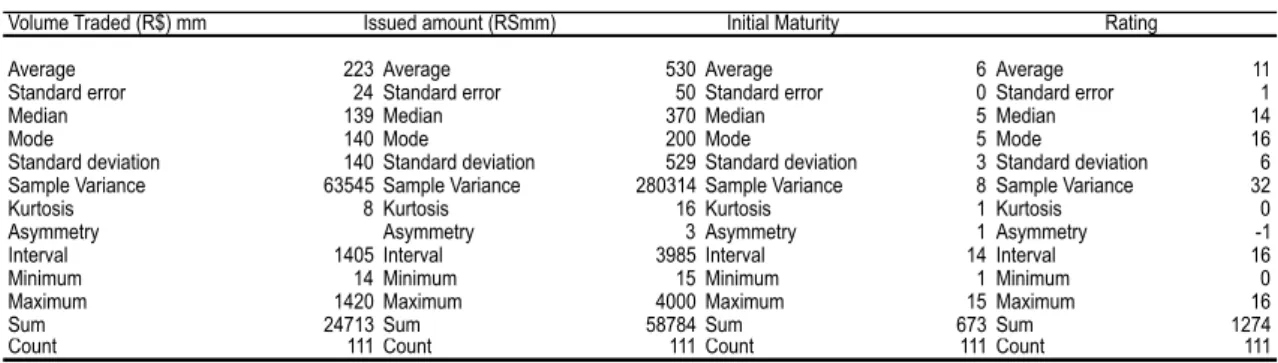
Table 4 Summary of Debenture Sample 1
Source : Author
According to table 4, the average debenture was traded for a volume of R$ 223 mm had an issue amounting to R$ 529 mm and initial maturity of 6 years with A rating ( A rating according to Fitch and SP which is equivalent to an A1 rating for Moody’s). This means that in our sample of liquid debentures, on average, 40% of the volume of the debenture was traded over the 4 year period. This was expected as we selected the 50 most liquid debentures between 2010 and 2014 which had more chances of being large Brazilian companies with international recognition and ability to access foreign capital markets.
Nevertheless, we note that certain sectors such as Leasing and Concession have lower chances of having a Eurobonds than other categories. This could be due to the already existing
Type of issuer
Concession Telecom Other Energy Real Estate Leasing Consumer Total Weighted Average
Number of issues Total Volume Issued (R$mm)
Average Initial Maturity
Percentage of Eurobonds
26 10 647 6,3 73%
12 11 426 6,8 100%
13 4 217 5,4 62%
31 18 736 6,7 77%
13 3 747 5,4 100%
10 7 474 5,1 20%
6 2 537 4,7 100%
111 58 784 -
-- - 6,1 76%
possibility of issuing long maturity and large bonds on shore. Indeed we see that the energy and concession sectors had one of the highest initial maturities with 6.7 and 6.8 years respectively. The highest issued debenture had a value of R$ 4,000 mm. This debenture was a 2006 issue of Vale Doce do Rio company and was the second most traded debenture over the 2010-2014 period just after a debenture from Concessionaria Rodoviaria do Tiete. The lowest issued debenture has a value of R$ 15 mm and was issued by Ouro Verde in 2014. This debenture was amongst the 10 least traded security in our sample over the period 2010-2014.
In terms of initial maturity we see from table 5 a high concentration of debentures that are concentrated below the 5 years range 60.4% and 31.5% between the 5 and 10 year range showing that most debenture are still short to medium term instrument. It is interesting to note that as times goes by the average maturity for debenture in our samples increases as showcased in table 5. The assimetricity is 1, meaning that data is pretty much equally distributed on both side of the mean and median (Table 5).
For issued amount we see a high concentration of issues (89.2%) below R$ 1,000 mm. Only 1 debenture was between the R$ 2000-3000 mm range and only one debenture was between the R$ 3000-4000mm range. These outliers cause the mean to be skewed to the right versus the median and the Asymmetry to be positive at 3.1.The fact that the data is slightly skewed to the right (assimetricity of 3) makes sense as no issue can be negative and some very high issue will tend to push the median to the right of the mean (Table 5).
Table 5 Descriptive Analysis of Sample 1 (111 debentures)
Source: Author
Graph 3 Frequency Distribution for Initial Maturity (Sample 1)
Source: Author
Graph 4 Maturity in function of Year (Sample 1)
Source: Author
Volume Traded (R$) mm Issued amount (RSmm) Initial Maturity Rating
Average 223 Average 530 Average 6 Average 11
Standard error 24 Standard error 50 Standard error 0 Standard error 1
Median 139 Median 370 Median 5 Median 14
Mode 140 Mode 200 Mode 5 Mode 16
Standard deviation 140 Standard deviation 529 Standard deviation 3 Standard deviation 6 Sample Variance 63545 Sample Variance 280314 Sample Variance 8 Sample Variance 32
Kurtosis 8 Kurtosis 16 Kurtosis 1 Kurtosis 0
Asymmetry Asymmetry 3 Asymmetry 1 Asymmetry -1
Interval 1405 Interval 3985 Interval 14 Interval 16
Minimum 14 Minimum 15 Minimum 1 Minimum 0
Maximum 1420 Maximum 4000 Maximum 15 Maximum 16
Sum 24713 Sum 58784 Sum 673 Sum 1274
Count 111 Count 111 Count 111 Count 111
60,4%
31,5%
8,1%
Below 5 Between 5 and 10 Between 10 and 15
Year Average maturity
2010 4.9
2011 5.2
2012 6.7
Graph 5 Frequency Distribution for Issued Amount in Million Reais (Sample 1)
Source: Author
Graph 6 Frequency Distribution for Ratings (Sample 1)
Source: Author
4.1.2 Descriptive analysis of Debenture sample 2
Sample 2 is composed of the 50 most traded debentures on a yearly basis, based on number of trades and contains 122 debentures that are divided amongst 7 sectors. The sectors that are most represented are the energy and other sectors with 29% and 18% of the issues respectively. The sectors for which there is high percentage of Eurobonds are Telecom, Real Estate and
Table 6 Summary of Debenture (Sample 2)
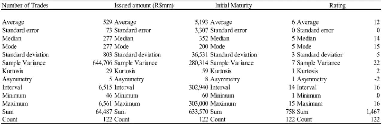
According to table 7, the average debenture was traded an average of 528 times over the 5 year period, had an issue amounting to R$ 5193 mm and initial maturity of 6.2 years with A+ rating. According to graph 7 we see that there is an overlap between the sample 1 and sample 2 as securities that trade a lot tend to have high volume. Nevertheless it was necessary to include those 2 samples as a security that trades a lot for a very little volume does not truly represent liquidity neither does a security that trades once for a high volume (In the latter case the holder would only have one “liquidity moment” to sell his stake). According to graph 7 43% of the debentures in this sample were not present in sample 1 which seems significant to potentially alter the results of the regression analysis.
From table 7, we see that the highest volume issued debenture had a value of R$ 303,000 mm. This debenture was a 2010 issue of Camargo Correa. Unlike in sample 1, this security traded very poorly being the 2nd least traded security in terms of numbers of trade. The lowest issued debenture has a value of R$ 60 mm and was a 2009 issue from Energisa Minas Gerais. Initial maturity showed an asymmetry of 1, meaning the data is pretty much evenly distributed on both sides of the mean.
For issued amount there is again a high concentration of issues 87.7% below R$ 1000 mm. Only 2 debentures are above the R$ 4000 mm threshold while 1 debenture is in both the 2000-3000 range and 3000-4000 range. The asymmetry is very strong, therefore the mean is much more skewed to the right 5193 than the median of 352 (Table 7).
For ratings similar distribution is observed from sample 1 with a slightly lower number of debentures in the 14-16 range (AA-AAA range) and with more debentures below the A+ rating. The distribution was the following: 43.52% between AA-AAA, 28.70% between A+ and AA and 27.78% below A+ (Graph 9.1).
Type of issuer
Concession Telecom Other Energy Real Estate Financial Consumer Total Weighted Average
Number of issues Total Volume (R$mm) Average Initial Maturity Percentage of Eurobond
23 9 757 7,5 83%
12 11 508 6,1 100%
22 276 799 5,5 64%
36 20 484 6,2 89%
13 305 919 5,9 100%
8 6 049 5,8 25%
7 2 374 5,6 100%
121 632 890 -
Table 7 Descriptive Analysis of Sample 2 (122 debentures)
Source: Author
Graph 7 Overlap Analysis (Sample 2)
Graph 8 Frequency Distribution for Initial Maturity (Sample 2)
Source: Author
Number of Trades Issued amount (R$mm) Initial Maturity Rating
Average 529 Average 5,193 Average 6 Average 12
Standard error 73 Standard error 3,307 Standard error 0 Standard error 0
Median 277 Median 352 Median 5 Median 14
Mode 277 Mode 200 Mode 5 Mode 15
Standard deviation 803 Standard deviation 36,531 Standard deviation 3 Standard deviation 5 Sample Variance 644,706 Sample Variance 280,314 Sample Variance 7 Sample Variance 22
Kurtosis 29 Kurtosis 59 Kurtosis 1 Kurtosis 2
Asymmetry 5 Asymmetry 8 Asymmetry 1 Asymmetry -2
Interval 6,515 Interval 302,940 Interval 14 Interval 16
Minimum 46 Minimum 60 Minimum 1 Minimum 0
Maximum 6,561 Maximum 303,000 Maximum 15 Maximum 16
Sum 64,487 Sum 633,570 Sum 758 Sum 1,467
Count 122 Count 122 Count 122 Count 122
Sample 1 that is different from
sample 2 43% Sample 1
debentures that are also part of
sample 2 57%
53,3%
38,5%
8,2%
Graph 9 Frequency Distribution for Issued Amount in Million Reais (Sample 2)
Source: Author
Graph 9.1 Frequency Distribution for Ratings (Sample 2)
Source: Author
4.2 Regression analysis
4.2.1 Regression of Debenture sample 1
Table 8 Correlation Matrix (Sample 1)
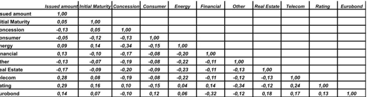
Before performing our regression analysis we checked for any multicollinearity amongst the independent variables (Table 8). This test is important as it shows if a relationship exists amongst the independent variable that could damage the interpretation of the model. For example if independent variable x1 is highly correlated to another variable x2 it is harder for us to predict the effect that one unit change in x1 will have on y as x1 will also impact x2. By looking at the table below, we see that rating and issued amount have a correlation of 0.29 which is relatively low. According to Anderson and Sweeney (2007) correlations below the 0.70 levels do not indicate multicollinearity issues likely to have a negative impact our regression model.
We then performed a regression analysis that includes all the independent variables (Table 8). The independent variables are Issued amount, Initial Maturity, Concession, Consumer, Energy, Financial, Other, Real Estate, Retail, Telecom, Utilities, Rating and Eurobonds. In this raw model the R2 is 0.59 and the R2 adjusted is 0.54 meaning that knowing X will help predict Y up to 54%.
Table 9 Regression Multiple (Sample 1)
Issued amount Initial Maturity Concession Consumer Energy Financial Other Real Estate Telecom Rating Eurobond Issued amount 1,00
Initial Maturity 0,05 1,00
Concession -0,13 0,05 1,00
Consumer -0,05 -0,12 -0,13 1,00
Energy 0,09 0,14 -0,34 -0,15 1,00
Financial 0,13 -0,10 -0,17 -0,08 -0,20 1,00
Other -0,13 -0,07 -0,19 -0,08 -0,22 -0,11 1,00
Real Estate -0,17 -0,09 -0,20 -0,09 -0,23 -0,11 -0,13 1,00
Telecom 0,28 0,08 -0,19 -0,08 -0,22 -0,11 -0,12 -0,13 1,00
Rating 0,29 0,16 0,10 -0,15 0,04 0,14 -0,34 -0,12 0,24 1,00
Source: Author
The coefficient of this regression were negative for certain economic sectors as well as ratings suggesting these variables have a negative relationship with the dependent variable. The negative relationship with the variable rating goes against the belief that investors tend to trade safer brazilian securities due to the the fragility of the institutions and the higer level of risk. In Sheng´s study (2004), ratings were expected to have a positive relationship with liquidity even though the link was not significant in any of the regression at the 5% level. Initial maturity, Issued amount, certain economic sectors as well as Eurobond had a positive relationship with the dependent variable. These positive signs are consistent with the work from previous authors. Amihud and Mendelson (1991) as well as Crabbe and Turner (1995) have both provided
argument for this positive coefficient. The first argument being linked to the likelihood of smaller issues being locked in a portfolio strategy, the second argument being that smaller issues translate into smaller availably and scrutiny of information. The Eurobond sign of the coefficient confirms our intuition that having a eurobond brings additional liquidity to the local debenture.
From Table 9 we observe that majority of independent variables have P values considerably above the 0.1 level. Rating and Eurobond are significant at the 0.05 level whereas Initial maturity and concession are only significant at the the 0.1 level.
The interpreation of the results for the significant independent variables are the following:
• For an increase in 1 year in initial maturity the average volume traded will increase by R$ 22 mm.
• A decrease in 1 point in ratings (A to A-) will increase the average volume traded by R$ 8.3 mm.
• Eurobond that is a binary variable needs to be interpreted in a different way as it does not show the marginal effect of adding one unit. The interpretation for this variable is that a debenture with a Eurobond will have on average R$ 95 mm more volume traded. Finally we need to check that the model has equal statistical variances (homoscedasticity) and that the residual values of the model are normally distributed. An ideal regression model should have a random dispersion of its residual values. If this is not the case this means there is still some explanatory power that has not been captured by the independent variables.
Graph 10 Breush Pagan and Koenker Tests for Heteroscedasticity (Sample 1)
Source: Author
We perform the Breush Pagan and Koenker tests to determine if the homoscedasticity
assumption is valid in our sample size. In both cases, the null hypothesis (H0) is that the sample presents homoscedasticity.
Graph 11 Robust Regression (Sample 1)
Source: Author
Using the robust regression model on SPSS, we observe that the coefficients stay the same but that new (hesterodesticity consistent) standard errors have been calculated. Initial Maturity for example that had a standard error value of 5,8 and a P value of 0,000 now has a (HC) standard error of 11,1 and a P value of 0,0536. At the 10% level we observe that Initial Maturity, Issued Amount, Rating and Eurobond are significant therefore the interpretation of the results still holds.
4.2.2 Regression of Debenture (sample 2)
Table 11 Correlation Matrix (Sample 2)
Issued amount (RSmm)Initial MaturityConcessionConsumer Energy Financial Other Real EstateTelecom Rating Eurobond Issued amount (RSmm) 1,
The correlation matrix in sample 2 does no suggest any problem with multicollinearity amongst the independent variables as the highest correlation other with rating (-0.44) and Eurobond with Financial are both below the (0.7) level.
Table 12 Regression Multiple (Sample 2)
Source: Author
I again performed a regular regression analysis on sample 2 to observe the coefficients for the dependent variables (Table 12). In this raw model the R2 is 0.25 and the R2 adjusted is 0.17 meaning that knowing X will help you predict only 17% of Y.
In this second regression the indepedent variable rating had negative relationship with the dependent variable. The independent variable Issued amount althought it has a very low coefficient of -0,001 has a negative coefficient in regression 2 which goes agains the findings from the existing litterature review. All the other independent variables had positive relationship with the number of trade variable, including Telecom, Real Estate and Consumer that had negative signs in regression 1.
From Table 12, we observe that only the variable initial maturity is significant at the 0.1 level and no variables has any significance at the 0.05 or 0.01 level. The interpreation of the results for the significant independent variable is the following:
• An increase in one year of Initial Maturity increases the number of trades by 116. Regression Statistics
R 0,50
R square 0,25
R square adjusted 0,17
Standard Error 729,37
Sample size 122,00
Coefficients Standard Error Stat t P Value H0 Rejected Interception -708,314 800,269 -0,885 0,378
Issued amount (R$mm) -0,001 0,002 -0,663 0,508 Initial Maturity 116,337 26,114 4,455 0,000 ***
Concession 771,160 746,663 1,033 0,304 Consumer 372,540 780,617 0,477 0,634 Energy 344,537 740,208 0,465 0,643 Financial 640,190 788,124 0,812 0,418 Other 409,580 756,880 0,541 0,590 Real Estate 294,339 758,663 0,388 0,699 Telecom 363,784 759,902 0,479 0,633 Rating -13,642 17,217 -0,792 0,430 Eurobond 284,820 201,933 1,410 0,161
Ho Rejected
We again check for any heteroskedasticity issues and non normal distribution of residual values in table 13.
Table 13 Breush Pagan and Koenker Tests for Heteroscedasticity (Sample 2)
Source: Author
For the second time, the P values of both tests are below 0,1 therefore we again reject the null hypothesis which means there is heteroscedasticity issues in our sample. This implies that the standards errors associated with the beta weights are not accurate and that they need to be recalculated using a more robust regression.
From this new robust regression we observe that the majority of standard errors have increased as well as the p values. For example Consumer that had a standard error of 780 and a P value of 0,634 now has a (HC) standard error of 808 and a P value of 0,64. As one can see, with the increase in P values in most cases the robust regression makes it harder for an independent variable to be significant in the regression. At the 10% level we observe that Initial Maturity and Eurobond are significant. This differs from the multiple regression in which only Initial
maturity was significant.
In most cases, robust standard errors and robust p values tend to be higher than in the non robust regression. However, in cases in which the variance of the error terms tends to be lower when x is far from its mean, standard error will tend to be large and robust standard errors will tend to be smaller than standard errors.
4.3 Analysis of Results
4.3.1 Results from the regression analysis
First it is important to clearly understand the limitations of the analysis to have a better understanding of the overall results.
The first limitation has to do with the selection of the sample. In this work, I have selected my sample based on the 50 most liquid debentures on an annual basis, therefore we can say that the results only are applicable to the most liquid securities and the proxies found after performing our regression analysis will not be helpful in explaining increase in liquidity for securities that trade once or twice per year. This first limitation has also an implication on the significance of the binary variable Eurobond. As seen in table 1 and 6 the proportion of our sample that also have Eurobonds is very high.
Table 15 Summary of Results of the Robust Regression Analysis
Source: Author
We note that the R2 in regression 2 is much lower than in regression 1 which has a high predictive value of 58%.
Comparing the results of this research with that of Sheng (2008), we observe that issued amount is confirmed as a good liquidity proxy and that hypothesis that having a Eurobond enables the debenture to gain in attractivity and expand its investor base. This result converges with the relationship found by Sanvicente (2001) between liquidity and ADR’s and more work could be done to understand the causes of this relationship.
The results of this study should be helpful for investors looking for tools to analyze liquidity of debentures and understanding the impact of Eurobonds on liquidity. Corporations should also benefit from the results of this study as they should start considering the positive effect of issuing Eurobond on their debentures when deciding to raise capital.
5 Conclusions
To conclude, the relationship between initial maturity, issued amount, Eurobond, rating and liquidity was confirmed although only Initial maturity and Eurobond were significant in both regressions.
From our results it seems that investors have a clear preference for debentures that have Eurobonds, as it was significant in both robust regressions. (In robust regression 1 at the 1% confidence level and in robust regression 2 at the 5% confidence level). Having access to the investor base of the bonds would be very helpful in understanding the overlap that exists between holders of Eurobonds and holders of debentures for the same company. This information could explain if the increase in liquidity is due to interest from new investors. Secondly, our results seem to indicate that the Eurobond market is complimentary and beneficial to the local Brazilian debenture market. This goes against the view that Eurobonds could be harmful to the development of the local debenture market by taking away liquidity. Another important point is that our results only show characteristics that help explain liquidity in the debenture market. From our results we cannot make conclusions for the liquidity premiums of the dependent variables.
Our findings for the Eurobond proxy could lead to the following future research:
o Does the time of the issue of Eurobond matter ? ( Does it the issue need to be recent, does the issue of Eurobond need to be before the debenture)
6 REFERENCES
Alexander, G. J., Edwards, A. K., & Ferri, M. G. (2000). The determinants of trading volume of high-yield corporate bonds. Journal of Financial Markets, 3(2), 177-204.
Amihud, Y., & Mendelson, H. (1991). Liquidity, asset prices and financial policy. Financial Analysts Journal, 56-66.
Anderson, R. W., & Sundaresan, S. (1996). Design and valuation of debt contracts. Review of financial studies, 9(1), 37-68.
Black, S., & Munro, A. (2010). Why issue bonds offshore?. Thursday 6 August 2010, 97.
Chordia, T., Roll, R., & Subrahmanyam, A. (2008). Liquidity and market efficiency. Journal of Financial Economics, 87(2), 249-268.
Chordia, T., Sarkar, A., & Subrahmanyam, A. (2005). An empirical analysis of stock and bond market liquidity. Review of Financial Studies, 18(1), 85-129.
Crabbe, L. E., & Turner, C. M. (1995). Does the liquidity of a debt issue increase with its size? Evidence from the corporate bond and medium-‐term note markets. The Journal of Finance, 50(5), 1719-1734.
Diaz, A., & Navarro, E. (2002). Yield spread and term to maturity: default vs. liquidity. European Financial Management, 8(4), 449-477.
Elton, E. J., & Green, T. C. (1998). Tax and liquidity effects in pricing government bonds. The Journal of Finance, 53(5), 1533-1562.
Elton, E. J., & Gruber, M. J. (2000). Corporate Bonds.
Fleming, M. J. (2002). Are larger treasury issues more liquid? Evidence from bill reopenings. Journal of Money, Credit and Banking, 707-735.
Gehr Jr, A. K., & Martell, T. F. (1992). Pricing efficiency in the secondary market for investment-grade corporate bonds. The Journal of Fixed Income, 2(3), 24-38.
Giacomoni, B. H., & Sheng, H. H. (2013). The impact of liquidity on expected returns from Brazilian corporate bonds. Revista de Administração (São Paulo), 48(1), 80-97.
Gozzi, J. C., Levine, R., Peria, M. S. M., & Schmukler, S. L. (2012). How firms use domestic and international corporate bond markets (No. w17763). National Bureau of Economic Research.
Houweling, P., Mentink, A., & Vorst, T. (2005). Comparing possible proxies of corporate bond liquidity. Journal of Banking & Finance, 29(6), 1331-1358.
Jankowitsch, R., & Pichler, S. (2002). Parsimonious estimation of credit spreads. Available at SSRN 306779.
Mahanti, S., Nashikkar, A., Subrahmanyam, M., Chacko, G., & Mallik, G. (2008). Latent
liquidity: A new measure of liquidity, with an application to corporate bonds. Journal of Financial Economics, 88(2), 272-298.
Mendelson, M. (1972). THE EUROBOND AND CAPITAL MARKET INTEGRATION*. The Journal of Finance, 27(1), 110-126.
Mullineaux, D. J., & Roten, I. C. (2002). Liquidity, Labels and Medium-‐Term Notes. Financial Markets, Institutions & Instruments, 11(5), 445-467.
Pimentel, R. C. (2006). O mercado de eurobonds e as captações brasileiras: Uma abordagem empírico-descritiva (Doctoral dissertation, Universidade de São Paulo).
7 APPENDIXES
7.1 Appendix 1: Sample 1 Debenture
Code Volume Traded (R$mm) Issued amount (R$mm) Initial
Maturity Sector Rating Eurobond
Issued Year
CVRD27 1365 4000 7 Energy 16 1 2006
TNLE15 750 1754 4 Telecom 16 1 2010
CVRD17 576 1500 4 Energy 16 1 2006
ITSP22 506 749 5 Financial 16 0 2007
BRTO29 434 1600 8 Telecom 16 1 2012
TLNL11 411 1620 5 Telecom 16 1 2006
TAEE33 400 702 12 Energy 16 1 2012
VIVO24 396 640 10 Telecom 16 1 2009
ANHB14 356 965 5 Concession 16 1 2012
TSPP22 355 800 10 Telecom 16 1 2005
ITSP12 339 751 3 Financial 16 0 2007
AMBV21 304 1248 6 Consumer 16 1 2006
TAEE13 272 665 5 Energy 16 1 2012
TLNL24 211 2035 3 Telecom 16 1 2009
TAEE23 208 793 8 Energy 16 1 2012
BNDP24 114 610 6 Financial 16 0 2009
ECRV11 105 461 4 Concession 16 1 2009
BNDS35 99 525 7 Financial 16 0 2010
BNDP36 87 1289 7 Financial 16 0 2012
VIVO34 70 72 10 Telecom 16 1 2009
ANHB15 69 450 5 Concession 16 1 2013
PETR12 61 750 10 Energy 16 1 2002
BNDP12 41 500 6 Financial 16 0 2006
VIVO14 32 98 10 Telecom 16 1 2009
TLNL14 26 964 2 Telecom 16 1 2009
PETR13 19 775 8 Energy 16 1 2002
TIET11 491 900 5 Concession 15 1 2010
CMTR12 484 1566 2 Energy 15 1 2010
ELSP19 299 250 13 Energy 15 1 2005
SBSP1A 293 810 5 Utilities 15 1 2010
TEEP11 274 491 5 Energy 15 1 2009
CMTR33 223 670 10 Energy 15 1 2012
SBSP2A 203 405 3 Utilities 15 1 2010
ELSP12 187 400 4 Energy 15 1 2010
TRAC13 163 600 2 Energy 15 0 2009
Code Volume Traded (R$mm) Issued amount (R$mm) Initial
Maturity Sector Rating Eurobond
Issued Year
IVIA11 153 308 5 Concession 15 0 2010
CMTR23 148 200 7 Energy 15 1 2012
CMTR13 112 480 5 Energy 15 1 2012
GASP23 66 269 5 Energy 15 1 2013
GASP33 60 142 7 Energy 15 1 2013
BPAR22 47 660 2 Financial 15 1 2009
BPAR12 14 140 1 Financial 15 1 2009
ENPP13 1108 800 10 Energy 14 0 2006
TELE28 511 460 7 Telecom 14 1 2008
CCCI12 500 1000 10 Other 14 1 2012
TSAE22 442 367 7 Concession 14 1 2013
VFIN14 347 1250 10 Financial 14 0 2005
TELE18 347 1150 5 Telecom 14 1 2008
IGTA12 241 330 5 Real Estate 14 1 2011
BRPR11 197 369 5 Real Estate 14 1 2012
APAR12 161 232 4 Energy 14 1 2009
AVIA11 139 285 5 Concession 14 1 2010
CMDT33 120 654 12 Energy 14 1 2013
BRPR21 79 231 7 Real Estate 14 1 2012
LSEL16 62 250 2 Energy 14 1 2009
AVIA21 61 120 7 Concession 14 1 2010
RDVT11 1420 1065 15 Concession 13 1 2013
ECOV22 739 681 11 Concession 13 1 2013
CVIA11 253 286 5 Concession 13 0 2010
GEPA14 198 250 5 Energy 13 1 2013
CYRE22 192 250 10 Real Estate 13 1 2008
ECOV12 164 200 7 Concession 13 1 2013
CCRD15 92 350 3 Concession 13 1 2009
ALGA22 87 233 7 Telecom 13 1 2012
VIAN11 80 154 5 Concession 13 0 2010
CVIA21 51 120 7 Concession 13 0 2010
ELTR12 49 50 7 Energy 13 0 2007
SUZB13 44 333 10 Other 13 0 2004
VIAN21 33 100 7 Concession 13 0 2010
AEPA13 28 190 3 Other 13 1 2009
CART12 578 380 12 Concession 12 1 2012
BRML21 179 270 9 Real Estate 12 1 2007
MRVE16 141 500 5 Real Estate 12 1 2012
GFSA18 95 288 5 Real Estate 12 1 2010
VOES13 74 150 4 Concession 12 0 2011
Code Volume Traded (R$mm) Issued amount (R$mm) Initial
Maturity Sector Rating Eurobond
Issued Year
CART22 59 370 12 Concession 12 1 2012
MRVP15 46 500 5 Real Estate 12 1 2011
BISA23 42 150 5 Real Estate 12 1 2011
BISA13 30 150 4 Retail 12 1 2011
SBSP29 22 120 7 Utilities 12 1 2008
HYPE13 21 201 4 Consumer 12 1 2010
SBSP19 17 100 5 Utilities 12 1 2008
DASA12 293 700 5 Other 11 1 2011
ENSE12 32 60 5 Energy 11 0 2009
TRIS11 31 200 5 Real Estate 11 1 2008
OVTL22 30 15 5 Other 11 1 2011
ALLG18 263 539 5 Other 10 1 2011
RDNT12 156 200 5 Concession 10 0 2010
HYPE23 48 336 5 Consumer 10 1 2010
HYPE33 32 114 6 Consumer 10 1 2010
CROD32 750 750 5 Concession 0 1 2011
BNDS25 486 1000 4 Financial 0 0 2010
CROD22 479 550 4 Concession 0 1 2011
LSVE17 372 650 5 Energy 0 1 2011
GLEX13 340 400 3 Consumer 0 1 2012
AMLP33 217 151 5 Other 0 0 2010
LDCS11 213 600 15 Energy 0 0 2009
AMLP23 160 300 4 Other 0 0 2010
CPCO11 136 165 2 Energy 0 1 2009
AMLP13 109 300 3 Other 0 0 2010
OAEP15 107 209 3 Real Estate 0 1 2012
MRSS15 73 300 6 Other 0 1 2012
CPTE11 67 220 12 Energy 0 1 2011
ENMG17 66 60 5 Energy 0 0 2009
AGUT12 65 400 2 Real Estate 0 1 2012
SAEL11 62 80 5 Energy 0 0 2009
ATDC11 60 90 5 Other 0 1 2012
AMLP43 48 149 5 Other 0 0 2010
MRFG23 40 238 4 Consumer 0 1 2011
7.2 Appendix 2: Sample 2 Debentures
Code Number of Trades
Issued amount (R$mm)
Initial
Maturity Sector Rating Eurobond
Issued Year
RDVT11
6561 1065 15 Concession 13 1 2013 ECOV22
3862 681 11 Concession 13 1 2013 CART12
3356 380 12 Concession 12 1 2012 CVRD27
2424 4000 7 Energy 16 1 2006 TNLE15
2095 1754 4 Telecom 16 1 2010 CBAN21
1590 550 14 Concession 13 1 2010 CBAN11
1561 550 14 Concession 13 1 2010 BRPR21
1555 231 7 Real Estate 14 1 2012 TPIS24
1455 392 5 Financial 0 1 2012 CMTR33
1428 670 10 Energy 15 1 2012 TIET11
1282 900 5 Energy 15 1 2010
UNDA22
1249 80 5 Other 10 1 2011
TSAE22
1180 367 7 Concession 14 1 2013 BRTO29
1089 1600 8 Telecom 16 1 2012 BNDP36
1016 1289 7 Financial 16 0 2012 LSVE17
968 650 5 Energy 0 1 2011
ENGI25
955 271 7 Energy 13 1 2012
IGTA12
881 330 5 Real Estate 14 1 2011 UNDA12
877 420 5 Other 10 1 2011
ALLG28
853 271 7 Other 10 1 2011
ALLG18
843 539 5 Other 10 1 2011
CMTR23
668 200 7 Energy 15 1 2012
ECOV12
652 200 7 Concession 13 1 2013 TAEE33
648 702 12 Energy 16 1 2012
AMLP33
632 151 5 Other 0 0 2010
DASA12
552 700 5 Other 11 1 2011
LRNE25
536 80 7 Consumer 15 1 2012
HYPE33
529 114 6 Consumer 10 1 2010 BISA22
519 81 6 Consumer 12 1 2010
LRNE14
511 215 5 Consumer 15 1 2011 DVIX11
494 100 4 Energy 11 1 2012
TEEP11
493 491 5 Energy 15 1 2009
SBSP1A
484 810 5 Utilities 15 1 2010
VIVO24 469 640 10 Telecom 16 1 2009 CROD22
455 550 4 Concession 0 1 2011 PANA13
432 250 5 Other 11 0 2005
BNDS35