Integration options for mercosul - an investigation Uusing the AMIDA Model

(1)

No ₆₁₀ _{ISSN 0104-8910}

Integration Options for Mercosul – An

Investigation Using the AMIDA Model

Renato Galv ˜ao Fl ˆores Junior, Masakazu Watanuki

(2)

Os artigos publicados são de inteira responsabilidade de seus autores. As opiniões

neles emitidas não exprimem, necessariamente, o ponto de vista da Fundação

(3)

INTEGRATION OPTIONS FOR MERCOSUL – An Investigation

Using the AMIDA Model *

(Version 0+1: January 18, 2006)

Renato G. Flôres Jr.

EPGE / Fundação Getulio Vargas, Rio de Janeiro

Masakazu Watanuki

IADB / Integration Department, Washington, D.C.

(4)

1. Introduction.

The pace of the Doha negotiations and the events that took place in the past two

years in the external front of Mercosul announce that the second half of this

century’s first decade will witness a revival of regional initiatives. The WTO

Round will probably deliver a package of resolutions that, though always

important, are more likely to set key targets for future liberalisations, beyond

modest advances in the main trade areas. This will inevitably trigger a new push

for regional agreements to complement, or answer, quests that were on the table

in Geneva. For the Southern Cone, it is nearly a certainty that both negotiations

that have been put aside, the free trade areas (FTAs) with, respectively, the EU25

and the whole Western Hemisphere, will resume. The latter has already suffered

many changes, and may even take place in a direct agreement with the US.

But not only former discussions will re-emerge. There is at present

significant activity in South America – tied with recent and challenging political

developments – leading, through more than one route, to a closer integration of

the Southern sub-continent. At the same time, the US, while keeping its face in

the Free Trade Area of the Americas (FTAA), has signed several agreements

with Central and South American groups of countries that, in a way or other, will

change the direction of many trade flows. In fact, in the case of South American

countries, there is a sort of subdued competition between it and Mercosul, to see

which side will attract more partners, and gain first the commercial chunks lying

in third groups like the Andean Community (AC). Additional complexity is

provided by the increasing role of China, and the Asian continent in general, in

the world trade flows, affecting not only the major Northern blocs – EU25 and

NAFTA – but Mercosul as well, especially Brazil and Argentina.

All this calls for a re-evaluation of exercises performed some time ago,

together with the introduction of new scenarios. In this paper, we use a brand

new static CGE model, AMIDA – Analysing Mercosul’s Integration Decisions

and Agreements, to help in shedding light on this diversity of options and

(5)

The AMIDA – Analysing Mercosur’s Integration Decisions and

Agreements model1, in its present, first version, though containing two service

sectors for closing the structure of the economy, is more suitable for the analysis

of market access for goods. Refinements and improvements, as a better, modern

treatment of services, are planned, in order to encompass other important issues,

part of most agreements at stake. Though it uses perhaps the best available data

set on Mercosul’s world trade flows and barriers – a most crucial point for these

exercises –, continuous updating and use of more accurate information is also in

view.

The structure of the paper is the following. Section 2 contains a few lines

on methodological aspects related to the model, discussing also data sources and

decisions. Section 3 presents the sectoral aggregation, the regions and the

scenarios. Six FTAs have been the object of this study. Results are presented and

commented upon in section 4, while section 5 tries to use them to make a first

assessment of Mercosul’s potentialities and shortcomings. Section 6 concludes.

Conclusions deal with more technical aspects as well as those describing the

main policy guidelines that can be extracted from the work.

2. Brief description of the model and data.

2.1. Basic facts.

The model basic lines follow those in Flôres (1997, 2003), being a static,

computable general equilibrium (CGE) model in which strategic interaction takes

place in certain sectors. This means that, contrary to the common practice of

introducing ad hoc “scale gains” in an otherwise perfect competition CGE2,

perfect and (explicitly) imperfect competition sectors interact in the model. This

approach was fashioned in Gasiorek, Smith and Venables (1992) – drawing on a

1_{AMIDA, infinite light, is also a great Buddha who, in our bodies, occupies the mouth. The}

authors hope the model to be a voice that will help Mercosur in choosing the best agreements.

2_{For a discussion of this topic, and of the (usually) accompanying “dynamic elasticities” device,}

(6)

pioneer partial equilibrium structure by Smith and Venables (1988) -, who used it

to evaluate the impacts of the Europe 92 Delors’s initiative.

In general, due to the scale effects – enhanced in the larger markets

created by the regional integrations -, welfare gains are higher than those

produced by the perfect competition alternatives3. However, in all FTAs

examined here, like the FTAA or the EU25-Mercosul cases, country markets

remain segmented as what is at stake is the creation of free-trade areas and not a

common market. This means that the model solutions, for the imperfect

competition sectors, keep the segmented markets approach. The results, as

discussed in section 4, seem promising and point to patterns and effects unable to

be unveiled by other techniques.

Another important issue is that, beyond tariffs, Flôres (1997, 2003) and

Gasiorek, Smith and Venables (1992) assumed the existence of additional trade

costs which can be associated to a variety of factors, impairing or raising the cost

of trade between two countries, like transportation, bureaucracy, distribution

costs, etc. Integration zeroes the tariffs and reduces, without necessarily

eliminating, these latter costs. We estimated gross transport margins with the aid

of COMTRADE, minimising discrepancies with official statistics. In most

bilateral flows they amount to less than 10 per cent, though there are significant

differences at the sectoral level, due to inconsistencies and misreporting. We

reduced them between the partners, in each scenario, by 4 percentage points, at

most, as trade facilitation. No evaluation was made of other trade costs. This

does not mean that such improvement is not worth pursuing in further

simulations.

From the theoretical side, handling the two kinds of competition in a

single general equilibrium framework poses theoretical problems related to the

existence and uniqueness of solutions, fully discussed, for instance, in Chapter 11

of Ginsburgh and Keyzer (1997). In our particular case, the specifications used

3

(7)

guarantee the existence of a unique solution, and we shall not mention this

question hereafter.

Flôres and Watanuki (2005) provide a detailed description of the model

equations, carefully discussing their role and pros and cons. Calibration and data

issues are also addressed in detail. We shall, in the remaining of this section,

briefly outline some key points.

Firms in imperfect competition sectors are symmetric and play a

Cournot-Nash strategy in each market/region, a key parameter being the perceived

elasticity of demand in region i, for product j, manufactured in region i’, e(i’,i; j),

which is defined as:

1/e(i’,i; j) = 1/σ(i;j) + ( 1 - 1/σ(i;j) ) s(i’,i; j)

where σ(i;j) is the elasticity of substitution, in region i, between goods j from

different origins and s(i’,i; j) is region’s i’ market share for product j, in region i.

Introducing imperfect competition in the way done here allows for the

computation of both short and long run solutions. In the former, the number of

(identical) firms in each imperfect competition sector is kept constant, so that

profits can be different from zero in these sectors. In the latter, profits are

imposed to be zero, and the number of firms is adjusted to satisfy this condition.

The structure of the model allows it to portray distinct levels of regional

integration in a progressive scenario evaluation. It contains both standard and

innovative features, as the ones below4:

i) in the demand side there is a representative consumer with a

Dixit-Stiglitz-Spence CES utility function in an Armington-like tree structure;

ii) in the production side, perfect competition sectors have Cobb-Douglas

technologies;

iii) intermediate inputs are treated via a shortcut using the input-output (I-O)

coefficients;

(8)

iv) wages are flexible, as labour is assumed mobile among sectors, but the

(sector specific) capital remuneration rates are kept constant;

v) there is no money in the model;

vi) in equilibrium, different closures (“equilibrium” and “disequilibrium”

ones) can be applied;

vii) calibration is, in these models, much more delicate. A new strategy,

accommodating polynomial cost structures depicting the scale economies

effect in the imperfect competition sectors, added more flexibility to this

key operation.

Finally, the whole model is run in an easy, GAMS-like programming

language

2.2. The data set.

An outstanding Western Hemisphere Database, combining information from the

UN, Eurostat, OECD, TRAINS, US Trade Representative, CEPAL, the World

Bank, national statistical institutes and central banks, GTAP’s latest database and

the IDB was produced.

In order to have a minimum compatibility among the different sources, the

base year for all data refers to 2001, which was adapted to the regions and

particular features of the model. We consider this a fairly ideal decision, as 2002

and 2003 were not very representative years for Brazil and, especially, Argentina,

and much information for 2004 was still unavailable.

Production and demand structures received careful attention in the case of

Mercosul. A key element relates to the I-O matrices for Brazil and Argentina,

which feature in rather old versions in GTAP. The 1996 and 2000 versions,

respectively, were updated and inserted instead. Also, Armington elasticities

came from special sources for these two countries. Capital remuneration rates

were improved whenever possible.

The US, Mexican, AC, Japanese, Chinese and EU economic data were

(9)

Information on the complete protection structure is always debatable, even

if one sticks to the case of tariffs. Preferential tariffs – specially those originating

from trade agreements –, usually poorly depicted, had to be thoroughly reviewed

in cases like Mercosul. Given the importance of the other two key regions in the

model, the US and the EU, improvements on their protection structure were

made with the aid of data from the United States International Trade Commission

– USITC website and EUROSTAT and Messerlin (2001), respectively.

Data from INTAL/ALADI and recent studies conducted by IPEA in Brazil

were also useful complementary sources. At the level of detail of the present

study, many nuances and, sometimes, important tariff peaks either disappear or

are smoothed out when aggregated to produce a single figure for the sector.

Nevertheless, the fact that the protection structure was computed bottom-up,

easily allows to translate any detailed (8-digits) concession/restriction to the

aggregation level of the model.

3. Sectors, Regions and Scenarios.

3.1. Sectors and regions.

We aimed at an as comprehensive as possible world regionalisation and sectoral

disaggregation. The economies were decomposed into twenty-five sectors

distributed along six groups, namely5:

I. (Classical) Agriculture:

Wheat, corn and other grains (Grains)

Vegetables & fruits

Oil seeds & soybeans

Sugar

Coffee, rice & other crops (Coffee, rice & others)

Animal products

(10)

II. Agribusiness (ab):

Bovine meat #

Poultry meat #

Dairy products

Beverages & tobaccos (Bev. & tobacco) #

Vegetable oils

III. Energy:

Minerals

Energy products

IV. Light Manufactures:

Textiles & apparel (Text. & apparel)

Leather, wood & paper (Leather, wood, paper)

Other light manufactures (Other light manufac.)

V. Heavy Manufactures:

Chemical and plastic products (Chemicals & plastics)

Ferrous metals

Non-ferrous metals

Motor vehicles #

Other transport equipment (Other transp. equip.) #

Electric equipment

Machinery

VI. Services:

Utilities & construction

Trade and services.

The first five groups comprise the 23 trade-in-goods sectors which will be

the main focus of our analyses. Five out of them – those marked with an ‘#’

above – were modelled under imperfect competition. These structures are better

portrayed in the model regions related to the Mercosul countries, the US, Japan

(11)

Decisions on the regions must face one of the most classical dilemmas in

CGE practice: due attention to the areas of concern (and those which affect them)

together with care in not fragmenting too much the model, what, among other

practical problems, may add distortions to its construction and operation. Given

the interest in analysing several different scenarios from a Mercosul perspective,

we divided the world into the following ten regions:

0. Mercosul6

1. Mexico

2. the United States

3. the Andean Community (Bolivia, Colombia, Ecuador, Peru and

Venezuela)

4. the Rest of the Americas (or Western Hemisphere) – RoWH

(comprising the remaining 23 potential FTAA countries)

5. the EU25 countries

6. Japan

7. China

8. the Asian 10 emerging economies (Asia10)

9. the Rest of the World - RoW.

As regards the quality of the data adaptation to these regions, the best ones

seem to be, as mentioned, those for Mercosul, Mexico, the AC, the US, the EU25

and Japan. The Rest of the Western Hemisphere is naturally a simplification,

though it includes, beyond the whole Central America, countries like Canada and

Chile. Equilibrium flows to the Rest of the World may also be obtained by

difference and econometric techniques. In this last region, are found countries

that may be relevant for certain sectors, like Australia and New Zealand, or India.

All the (former) New Tigers – Hong Kong, Korea, Singapore and Taiwan -,

beyond six new emerging Asian economies, like Indonesia, Malaysia or

6 _{From this region, individual country results, if desired, can be extracted (see Flôres and}

(12)

Vietnam, which are becoming competitive either in specific agricultural goods or

in traditional sectors like textiles, are in Asia10.

Exhibit I shows, for Mercosul, the values of the trade flows, for the

twenty-three merchandise sectors, plus the services group. It is an essential tool

for understanding the scope of the model and the true meaning of the results

discussed in the next section.

Exhibit I: Mercosul: Trade flows – imports and exports, 2001 -, by regions (106

US$).

I.A: Exports (fob) [cont.] REGIONS SECTORS

1 2 3 4 5

Grains 19,0 3,0 191,6 155,5 301,4

Vegetables & fruits 210,7 2,7 18,2 54,7 797,0

Oilseeds & soybeans 26,1 44,4 116,4 52,6 2.312,9

Sugar 105,6 6,0 107,7 24,4

Coffee, rice & others 464,6 37,6 47,0 112,9 1.441,3

Animal products 838,0 53,0 207,5 271,7 1.976,7

Bovine meat (ab) 39,5 2,6 14,7 215,7 547,8

Poultry meat (ab) 186,7 5,3 18,9 828,8

Dairy products (ab) 33,9 94,7 55,0 29,9 0,5

Bev. & tobacco (ab) 62,0 9,8 15,6 36,9 91,2

Vegetable oils (ab) 39,0 1,3 256,6 221,6 3.653,7

Minerals 556,7 72,9 87,4 228,2 1.857,8

Energy products 639,1 1,4 61,0 2.104,2 226,9

Text. & apparel 357,0 49,8 158,8 152,6 329,2

Leather, wood, paper 3.306,2 188,2 215,3 512,3 2.438,9

Other light manufac. 115,9 11,4 27,1 24,7 48,8

Chemicals & plastics 1.033,9 204,6 745,4 732,6 954,0

Ferrous metals 1.382,3 154,9 303,6 275,8 695,5

(13)

Motor vehicles 1.356,0 1.142,6 593,8 445,0 931,1

Other transp. equip. 2.430,4 9,7 25,1 44,1 707,2

Electric equipment 1.417,6 104,7 131,3 136,9 213,9

Machinery 1.387,2 283,2 578,3 519,3 793,2

(Services) 2.166,4 139,5 85,5 515,4 5.839,4

TOTAL 19.035,4 2.682,9 4.081,0 7.175,7 27.849,2

I.A: Exports (fob) [end] REGIONS SECTORS

6 7 8 9

TOTAL

Grains 134,6 2,5 207,1 1.112,2 2.127,0

Vegetables & fruits 1,4 10,2 88,7 1.183,6

Oilseeds & soybeans 171,3 1.496,7 286,5 308,6 4.815,4

Sugar 0,2 25,1 106,1 1.639,2 2.014,3

Coffee, rice & others 194,0 88,3 84,4 423,1 2.893,1

Animal products 299,2 56,3 179,6 526,6 4.408,7

Bovine meat (ab) 7,4 1,0 103,1 324,1 1.255,9

Poultry meat (ab) 177,8 6,2 206,5 731,1 2.161,2

Dairy products (ab) 1,9 4,4 40,2 260,6

Bev. & tobacco (ab) 43,9 0,4 9,6 28,6 298,0

Vegetable oils (ab) 31,1 21,5 638,9 2.285,3 7.149,0

Minerals 716,9 668,4 336,0 668,2 5.192,4

Energy products 27,3 168,8 3.228,6

Text. & apparel 40,6 126,2 17,8 66,2 1.298,2

Leather, wood, paper 240,3 387,0 580,2 371,1 8.239,6

Chemicals & plastics 107,4 78,4 159,3 357,4 4.373,2

Ferrous metals 113,2 116,3 429,8 385,5 3.857,1

Non-ferrous metals 385,3 24,3 52,5 379,7 2.952,8

Motor vehicles 9,3 130,0 31,7 332,4 4.972,0

Other transp. equip. 0,8 60,9 18,9 256,1 3.553,2

(14)

Machinery 36,6 101,9 94,6 354,6 4.148,9

(Services) 837,2 205,6 1.552,5 2.159,8 13.501,3

TOTAL 3.586,0 3.651,3 5.157,9 13.064,5 86.283,8

I.B: Imports (cif) [cont.] REGIONS SECTORS

1 2 3 4 5

Grains 17,6 0,1 15,0 0,2

Vegetables & fruits 9,7 3,3 79,1 114,5 32,5

Oilseeds & soybeans 1,8 0,7 0,1 2,0 1,1

Sugar

Coffee, rice & others 38,4 0,7 13,3 13,6 48,7

Animal products 224,2 29,5 110,9 180,1 310,5

Bovine meat (ab) 4,9 2,3 3,7

Poultry meat (ab) 3,5 0,6 8,2 21,0

Bev. & tobacco (ab) 26,4 5,0 1,2 60,5 272,3

Vegetable oils (ab) 8,6 0,1 2,4 0,2 81,9

Minerals 166,9 21,1 105,3 298,6 381,5

Energy products 337,8 773,5 100,3 79,4

Text. & apparel 163,7 32,5 31,3 60,5 357,7

Leather, wood, paper 446,7 14,6 40,9 464,3 894,7

Chemicals & plastics 4.950,9 470,2 252,1 485,1 5.389,5

Ferrous metals 105,3 13,4 5,9 20,2 438,1

Non-ferrous metals 545,4 16,2 172,3 423,3 964,1

Motor vehicles 537,4 232,8 9,8 69,6 2.516,1

Other transp. equip. 2.075,4 0,7 92,1 951,9

Electric equipment 3.633,5 200,3 0,7 254,0 1.784,6

Machinery 5.211,3 147,8 58,3 292,8 7.367,9

(Services) 4.129,2 209,0 98,8 1.002,9 9.650,2

(15)

I.B: Imports (cif) [end] REGIONS SECTORS

6 7 8 9

TOTAL

Grains 0,7 33,4

Vegetables & fruits 10,5 3,3 28,2 281,2

Oilseeds & soybeans 0,1 1,1 6,9

Sugar

Coffee, rice & others 4,5 4,6 27,7 68,6 219,9

Animal products 5,8 21,4 53,2 257,3 1.192,9

Bovine meat (ab) 0,3 2,8 14,0

Poultry meat (ab) 0,2 0,4 33,8

Dairy products (ab) 21,0 77,5

Bev. & tobacco (ab) 0,4 0,1 0,8 42,7 409,3

Vegetable oils (ab) 0,1 33,4 11,8 138,4

Minerals 47,8 54,8 38,6 143,0 1.257,5

Energy products 42,6 185,6 27,4 2.399,6 3.946,1

Text. & apparel 18,4 302,7 597,2 368,0 1.932,0

Leather, wood, paper 23,6 177,0 149,3 117,4 2.328,5

Chemicals & plastics 532,5 550,4 805,6 2.582,7 16.018,9

Ferrous metals 68,6 23,0 59,4 186,5 920,4

Non-ferrous metals 143,8 117,0 111,5 263,0 2.756,6

Motor vehicles 847,5 8,2 301,7 307,7 4.830,8

Other transp. equip. 135,3 87,5 70,2 90,5 3.503,7

Electric equipment 807,1 644,8 2.110,5 735,9 10.171,5

Machinery 1.496,2 830,6 1.053,0 1.156,7 17.614,5

(Services) 699,7 297,4 2.614,2 2.948,1 21.649,5

TOTAL 4.907,6 3.611,4 8.157,8 11.770,8 90.119,6

3.2. The scenarios.

We tried to run a diversified set of scenarios to produce a global idea on the

(16)

naturally, the FTAs with, respectively, the US and the EU. Both can be

contrasted to the FTAA initiative – in its original form – as well as to a set of

alternatives, comprising different international positions Mercosul may assume.

Moreover, they should also be confronted with possible outcomes from the

present WTO Doha Round, what hasn’t been done in this paper7.

Five scenarios, which will be called basic, have then been defined. These

basic options may be translated into manifold ways as well as combined in

multiple forms. A sixth scenario, involving a FTA with China is also considered.

Out of the wide spectrum of possible combinations, the following will be

discussed here:

Scenario A. The first main scenario, in which Mercosul closes a full FTA

agreement with the US.

Scenario B. The second main one, with the EU25-Mercosul FTA fully

implemented.

Scenario C. This is a first “diversion”, with Mercosul signing a FTA with

Mexico.

Scenario D. A second diversion, Mercosul now closing a FTA with the Andean

Community, something that is already a reality on paper.

Scenario E. The classical implementation of the FTAA, meaning that all tariffs,

for all sectors, among all the regions comprising the American continent in the

model are zeroed.

Scenario F. This scenario includes a different option, analysing the impact of

Mercosul’s free trade with China.

Of course, it is also desirable to evaluate the impact of not-so-perfect

FTA’s, something that will be pursued later, following lines in Flôres (2003). At

present, supposing full FTAs are implemented in all cases allows a clearer cross

evaluation of them.

7 _{The main reason for this absence is that, even after the December 2005 Hong Kong}

(17)

4. Results.

Tables 1 to 14 are a selection of the most interesting results, they concentrate

initially on the impacts in the trade flows. All deserve careful analysis and will be

briefly discussed below. It is worth reminding – specially given the previous

remarks on the database and the aggregate level of the study – that all the figures

should be basically evaluated in relation to each other, within and between tables,

and not taken separately, as a precise single value for the changes. The

importance of this section is to identify areas or situations – or rather sectors and

scenarios – where things can go better or worse. Detailed quantification of profits

or losses should be made at a greater level of detail, ultimately with the aid of

partial equilibrium models8.

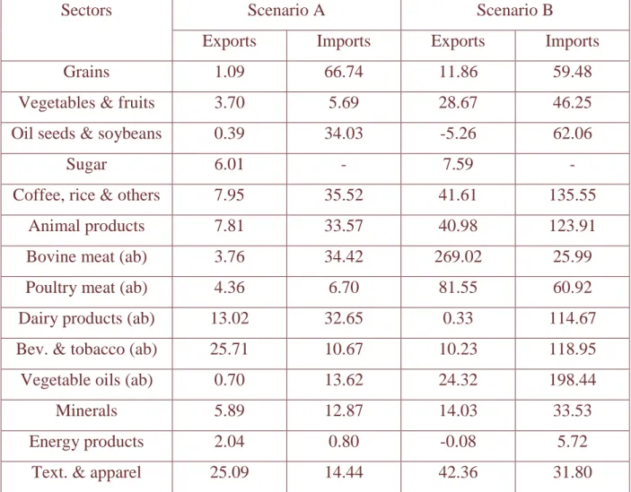
Table 1 describes the changes in trade flows under the two main scenarios.

Four out of the five highest increases for exports, in the EU25 scenario (B), are in

commodities (2) and agribusiness (2) sectors, the other being textiles & apparel.

In the US case, two heavy manufactures sectors appear, beyond one in the

agribusiness – thanks largely to orange juice - and two traditional ones, textiles

(again) included.

In a rough overall picture, the EU25 FTA seems to favour demand for

more traditional Mercosul’s exports, while the US one promotes some higher

value-added exports. The very protectionist European CAP - Common

Agricultural Policy shows itself indirectly in the significant increases in bovine

and poultry meat; US figures in the agribusiness sectors being more modest.

However, the EU25 remains competitive in this area and, either due to this, or to

compensate the demand surge in the EU, or both, Mercosul’s imports changes of

agricultural commodities and agribusiness are, but for two exceptions (grains and

bovine meat), considerably higher in the EU25 FTA. Indeed, this is also valid for

8_{Given all the methodological caveats already mentioned, we decided not to translate the results}

(18)

most of the remaining sectors, only exceptions being other transport equipment

and electric equipment.

At the bottom of the Table, the value of the correlation coefficients

between each two corresponding vectors is displayed (not including services).

Given the very high increase in bovine meat exports in Scenario B, the

coefficients, for exports, were computed with and without this sector. There is no

(linear) relation between the two exports patterns, while the imports ones show a

certain degree of common behaviour.

Nearly all these contrasting results may be partially explained by the more

open, in relative terms, US protectionist structure.

Table 1: Mercosul’s FTAs with the US and the EU25: Total trade flows changes

(long run results; exports and imports) under scenarios A and B.

Scenario A Scenario B

Sectors

Exports Imports Exports Imports

Grains 1.09 66.74 11.86 59.48

Vegetables & fruits 3.70 5.69 28.67 46.25

Oil seeds & soybeans 0.39 34.03 -5.26 62.06

Sugar 6.01 - 7.59 -

Coffee, rice & others 7.95 35.52 41.61 135.55

Animal products 7.81 33.57 40.98 123.91

Bovine meat (ab) 3.76 34.42 269.02 25.99

Poultry meat (ab) 4.36 6.70 81.55 60.92

Dairy products (ab) 13.02 32.65 0.33 114.67

Bev. & tobacco (ab) 25.71 10.67 10.23 118.95

Vegetable oils (ab) 0.70 13.62 24.32 198.44

Minerals 5.89 12.87 14.03 33.53

Energy products 2.04 0.80 -0.08 5.72

(19)

Leather, wood, paper 20.87 12.00 23.30 23.88

Other light manufac. 6.21 42.02 9.34 62.56

Chemicals & plastics 15.08 7.89 12.37 8.44

Ferrous metals 13.52 7.63 15.75 26.12

Non-ferrous metals 12.83 9.38 24.88 15.86

Motor vehicles 19.11 22.27 9.95 100.34

Other transp. equip. 26.05 41.32 4.42 25.21

Electric equipment 20.73 5.61 8.91 3.71

Machinery 16.35 11.61 18.26 15.76

(Services) 0.97 -1.10 -2.67 3.29

TOTAL 9.51 9.09 19.42 18.57

Correlation between the two patterns: i) Exports, -0.08 (without bovine meat), -0.21 (with bovine meat); ii) Imports, 0.27 .

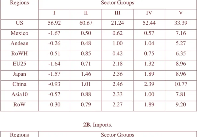
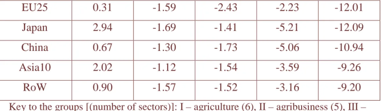
Tables 2 and 3 deepen the insight, showing the regional distribution of the

increases, according to the five groups of sectors9. Both regional agreements

present limited territorial externalities, with however certain nuances. The US

one seems to cause some efficiency gains in light and heavy manufactures

sectors, where Mercosul is able to increase exports to other areas in the world. In

the latter group, sensible increases take place in the three Asiatic regions, the

EU25 and the RoW. Nevertheless, the imports pattern is largely dominated by

very high penetration of the US flows, with, but for agricultural sectors,

decreases in the demand elsewhere. Though these are usually negligible, for the

two manufactures groups figures become again more significant, particularly for

heavy manufactures, exactly in the same five regions already mentioned. Very

clearly, the agreement will provoke trade deviation, in these sectors, from Asia

and the EU25 to US suppliers. A similar pattern, reasonably significant, also

takes place with the energy group.

9_{They can be complemented by tables showing the same information at the sector level. These,}

(20)

Increases in exports to the partner are usually more modest in scenario A

than in B. This very often also corresponds to lower absolute values.

Manufacturing groups IV and V sell, to the US, under scenario A, extra values of

1.98 bn US$ and 3.30 bn US$, respectively, while the much higher European

percentages under scenario B amount to 2.83 bn US$ and 3.55 bn US$,

respectively: a sizeable difference in the first case.

Table 2: Mercosul’s FTA with the US (Scenario A): Trade flows changes (long

run results) by Regions and Groups of Sectors.

2A. Exports.

Sector Groups Regions

I II III IV V

US 56.92 60.67 21.24 52.44 33.39

Mexico -1.67 0.50 0.62 0.57 7.16

Andean -0.26 0.48 1.00 1.04 5.27

RoWH -0.51 0.85 0.42 0.75 6.35

EU25 -1.64 0.71 2.18 1.32 8.96

Japan -1.57 1.46 2.36 1.89 8.96

China -0.93 1.01 2.46 2.39 10.77

Asia10 -0.57 0.88 2.33 1.00 7.81

RoW -0.30 0.79 2.27 1.89 9.20

2B. Imports.

I II III IV V

US 175.50 192.49 54.44 141.28 64.45

Mexico -0.56 -1.73 -2.74 -3.17 -9.06

Andean 0.39 -1.34 -1.58 -2.28 -7.55

(21)

EU25 0.31 -1.59 -2.43 -2.23 -12.01

Japan 2.94 -1.69 -1.41 -5.21 -12.09

China 0.67 -1.30 -1.73 -5.06 -10.94

Asia10 2.02 -1.12 -1.54 -3.59 -9.26

RoW 0.90 -1.57 -1.52 -3.16 -9.20

Key to the groups [(number of sectors)]: I – agriculture (6), II – agribusiness (5), III – energy (2), IV – light manufactures (3), V – heavy manufactures (7).

Table 3: Mercosul’s FTA with the EU25 (Scenario B): Trade flows changes

(long run results) by Regions and Groups of Sectors.

3A. Exports.

I II III IV V

US -17.08 -6.49 -3.51 -4.05 -2.09

Mexico -18.51 -2.75 -3.15 -2.84 -2.39

Andean -21.89 -8.28 -5.45 -0.96 1.02

RoWH -17.26 -5.71 -2.15 -3.05 1.52

EU25 79.72 144.99 54.04 100.41 69.21

Japan -26.65 -5.72 -11.30 -7.99 3.36

China -17.32 -16.08 -11.35 -8.14 3.75

Asia10 -21.28 -11.20 -11.89 -7.79 3.46

RoW -17.19 -8.89 -11.71 -7.68 2.40

3B. Imports.

I II III IV V

US 57.04 10.19 5.02 0.28 -9.82

Mexico 51.61 8.11 4.38 -0.34 -7.38

Andean 43.52 16.76 5.08 0.16 -6.89

(22)

EU25 312.61 201.38 86.58 117.17 73.11

Japan 66.33 9.35 2.18 -2.11 -10.72

China 49.09 8.21 5.12 -2.04 -8.97

Asia10 62.53 26.85 2.51 -0.78 -6.89

RoW 58.03 10.22 5.49 -0.41 -7.73

It is interesting to notice that the EU25 FTA pattern is nearly opposite to

the one depicted in Table 2. The considerable rise in exports to the EU takes

place at the expense of generalised decreases in all other regions, for every sector

but heavy manufactures in the Asian and RoW regions, plus the AC and the

RoWH. Imports, however, increase almost everywhere, exceptions being the

Asian regions and Mexico in light manufactures, and all destinations in heavy

manufactures, where – as happened in the US FTA - there is a clear trade

deviation in favour of the partner’s exports.

The combination of all results till now suggests a few things. First, both

FTAs with a Northern bloc will enhance Mercosul’s competitiveness in heavy

manufactures, very likely at the cost of inducing a considerable (though needed)

readjustment in this group of sectors. Second, while Scenario A transforms the

US into the major Mercosul supplier, in spite of probably also turning the

Southern Cone into a more competitive bloc, Scenario B strongly channels

Mercosul exports to the EU, in such a way that it is impelled to demand more

goods from all other regions. Clearly, this signals to the more distorting EU

protection structure, but also warns on the higher US dependency the sole

completion of Scenario A may entail.

The US Scenario A has two deviations and one deepening, the FTAA

itself. Table 4 shows the changes in the flows, by sectors groups, for Scenarios C

and D. The figures are more modest, though in the case of Mexico the increases

(23)

Community, on the other hand, shows its competitiveness in agriculture and

energy, where the highest changes in Mercosul’s imports take place.

Table 4: Mercosul’s FTAs with Mexico and the Andean Community: Total trade

flows changes (long run results; exports and imports) under scenarios C and D.

Scenario C Scenario D

Sectors Groups

Agriculture 0.36 5.02 2.72 16.02

Agribusiness 1.72 3.07 1.73 3.14

Energy -0.04 1.31 0.96 4.64

Light Manufactures 2.62 2.93 1.51 3.20

Heavy Manufactures 6.69 2.82 4.45 1.61

(Services) -0.89 1.06 -1.13 1.37

TOTAL 2.47 2.36 2.20 2.11

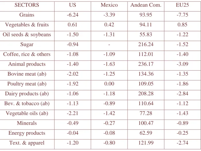
Table 5 gives a better, more detailed view of the dynamics of these

South-South integrations by displaying, for the four key regions, the sectoral changes in

the Andean Community FTA. The agreement causes deviation of Mercosul

exports in all other regions, though in general low; the highest one being,

uniformly, in the grains sector10. It dramatically unlocks Mercosul exports of

sugar, animal and dairy products, but the increases are significant for all sectors:

electric equipment, with 29.51 is the lowest one.

Contrasting imports and exports, evidences of intra-industry trade between

the two blocs emerge – at the aggregation level of the model –, in the areas of

beverages & tobacco, machinery, textiles & apparel, other light manufactures and

motor vehicles, among others. These last two sectors account for the highest

percentage increases in Andean exports to Mercosul. Indeed, they, together with

(24)

coffe, rice & other crops, animal products, vegetable oils and electric machinery,

there is an interesting evidence on the complementarities between the two blocs.

Of course, the Community becomes a main supplier of energy products to

Mercosul, negative though very small decreases taking place in all other regions.

The same applies, now again somewhat unexpectedly, with vegetables and fruits.

Apart from this, the FTA does not impact much the other regions’ exports.

Finally, the effects on the US and the EU25 are strikingly similar, as synthesised

by the two correlation coefficients.

Table 5: Mercosul’s FTA with the Andean Community: Total trade flows

changes (long run results; exports and imports), by the four main regions, under

scenario D.

5A. Exports.

SECTORS US Mexico Andean Com. EU25

Grains -6.24 -3.39 93.95 -7.75

Oil seeds & soybeans -1.50 -1.31 55.83 -1.22

Sugar -0.94 - 216.24 -1.52

Coffee, rice & others -1.08 -1.09 112.01 -1.40

Animal products -1.40 -1.63 236.17 -3.09

Bovine meat (ab) -2.02 -1.25 134.36 -1.35

Poultry meat (ab) -1.92 0.00 109.05 -1.86

Dairy products (ab) -1.06 -1.18 208.28 -2.84

Bev. & tobacco (ab) -1.13 -0.89 110.64 -1.12

Vegetable oils (ab) -2.21 -1.42 77.28 -1.43

Minerals -0.49 -0.27 100.47 -0.89

Energy products -0.04 -0.08 62.59 -0.25

Text. & apparel -1.20 -0.80 121.99 -2.74

(25)

Leather, wood, paper -1.24 -1.01 44.83 -2.29

Other light manufac. -0.10 -0.38 105.26 -1.78

Chemicals & plastics -1.75 -0.93 39.23 -1.72

Ferrous metals -1.56 -1.18 40.80 -3.47

Non-ferrous metals -0.99 -0.65 46.76 -2.26

Motor vehicles -0.37 -1.09 92.93 -0.89

Other transp. equip. -1.31 -1.48 135.58 -1.54

Electric equipment -1.03 -0.88 29.51 -2.03

Machinery -0.92 -1.43 72.64 -2.74

(Services) -1.23 -1.10 -2.89 -1.09

TOTAL -1.11 -1.08 76.93 -1.93

Correlation between the US and EU25 patterns (Exports), 0.84 .

5B. Imports.

Grains 10.48 - 136.54 9.46

Vegetables & fruits -2.37 -2.38 83.05 -2.43

Oil seeds & soybeans 3.37 3.61 170.06 2.58

Sugar - - - -

Animal products 2.98 3.01 146.95 2.88

Bovine meat (ab) 1.83 0.00 0.00 1.80

Poultry meat (ab) 1.97 0.00 70.22 1.95

Bev. & tobacco (ab) 1.52 1.53 182.32 1.48

Minerals 0.21 0.23 87.28 0.17

Energy products -0.46 - 21.15 -0.55

Text. & apparel 173 1.74 180.89 1.70

(26)

Ferrous metals 1.45 1.48 69.24 1.43

Motor vehicles 0.31 0.34 304.48 0.29

Other transp. equip. 2.87 2.90 0.00 2.82

Machinery 1.48 1.49 109.73 1.45

(Services) 1.38 1.39 2.87 1.36

TOTAL 1.22 0.92 52.39 1.16

Correlation between the US and EU25 patterns (Imports), 1.00 .

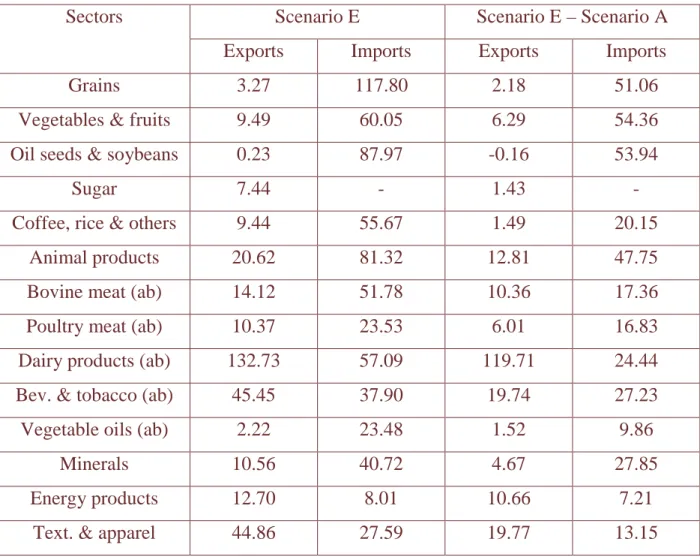
The FTAA, Scenario E, provides the integrated picture for scenarios A, C

and D, the US presence being responsible for a few non-linearities. Table 6 gives

a detailed picture of the total flows changes, for Mercosul. The two last rows

show the difference between these figures and the corresponding ones for

Scenario A, shown in Table 1; they reveal that the effects of Scenario A are

thoroughly enhanced.

Exports increases are usually superior in the full FTAA case, while

imports ones always. For exports, dairy products, motor vehicles, beverages &

tobacco, and textiles & apparel, in this order, present the greatest changes -

sectors where Mercosul, but perhaps for motor vehicles, clearly has an advantage

vis à vis more competitive blocs/economies. Notwithstanding, increases are also

positive in all remaining trade-in-goods sectors.

The pattern is somehow reverted in the imports flows, which increase

substantially in the agricultural group. However here percentage values can be

misleading. A 117.80 per cent rise in grains amounts to 39.3 m US$, while one of

15.45 per cent in machinery to 2.7 bn US$ !

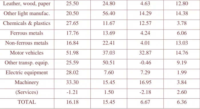
Tables 7 and 9 have formats similar, respectively, to Tables 2 and 5, and

allow for a closer examination of impacts. As expected, the FTAA induces

(27)

impact outside the hemisphere is somewhat negligible in the case of exports

(Japan even showing no decrease), for imports the changes are both uniform and

remarkable (notwithstanding increases in groups I and II). Table 8 adds a further

insight on this, by comparing the total flow changes for the four scenarios

dealing with WH integrations. From it, we see that the FTAA is as distorting –

with respect to regions outside the agreement – as the Mercosul-US FTA,

though, in the latter, Mercosul still increases its exports to all other regions.

Overall, the FTAA is roughly as beneficial to Mexico and the AC – in terms of

their trade relations with Mercosul – as the individual scenarios C and D. It is

undoubtedly a competitive choice within the realm of these four agreements.

Table 6: The FTAA: Total trade flows changes (long run results; exports and

imports) under scenario E, and differences E - A.

Scenario E Scenario E – Scenario A Sectors

Grains 3.27 117.80 2.18 51.06

Oil seeds & soybeans 0.23 87.97 -0.16 53.94

Sugar 7.44 - 1.43 -

Animal products 20.62 81.32 12.81 47.75

Bovine meat (ab) 14.12 51.78 10.36 17.36

Poultry meat (ab) 10.37 23.53 6.01 16.83

Bev. & tobacco (ab) 45.45 37.90 19.74 27.23

Minerals 10.56 40.72 4.67 27.85

Energy products 12.70 8.01 10.66 7.21

(28)

Other light manufac. 20.50 56.40 14.29 14.38

Ferrous metals 17.76 13.69 4.24 6.06

Motor vehicles 51.98 37.03 32.87 14.76

Other transp. equip. 25.59 50.51 -0.46 9.19

Machinery 33.30 15.45 16.95 3.84

(Services) -1.21 1.50 -2.18 2.60

TOTAL 16.18 15.45 6.67 6.36

Table 7: The FTAA (Scenario E): Trade flows changes (long run results) by

Regions and Groups of Sectors.

7A. Exports.

Sector Groups Total

Regions

I II III IV V

US 52.85 56.67 20.43 49.01 30.59 36.75

Mexico 118.19 200.92 112.50 163.88 116.40 124.65

Andean 106.44 89.79 94.40 75.29 43.01 61.54

RoWH 51.67 81.03 17.06 44.82 42.88 38.03

EU25 -4.01 -1.26 1.76 -2.82 5.18 -0.53

Japan -3.67 -0.42 2.56 -2.88 4.49 0.34

China -3.44 -2.17 2.60 -2.67 5.78 -0.66

Asia10 -2.97 -1.38 2.38 -3.11 2.22 -0.88

RoW -3.60 -1.08 1.38 -2.51 5.28 -0.67

7B. Imports.

(29)

I II III IV V

US 184.93 206.15 55.50 144.49 65.35 70.43

Mexico 210.90 231.57 115.74 202.07 105.18 113.18

Andean 136.61 223.08 28.47 131.36 56.91 55.59

RoWH 117.96 139.40 69.30 70.62 57.65 70.23

EU25 3.46 1.29 -3.60 -1.26 -11.69 -10.33

Japan 6.88 0.47 -2.44 -3.79 -12.07 -11.66

China 1.66 0.53 -0.23 3.68 10.16 -7.79

Asia10 5.47 2.72 -2.64 -2.35 -8.77 -7.43

RoW 4.01 2.29 0.69 -2.02 -8.75 -5.02

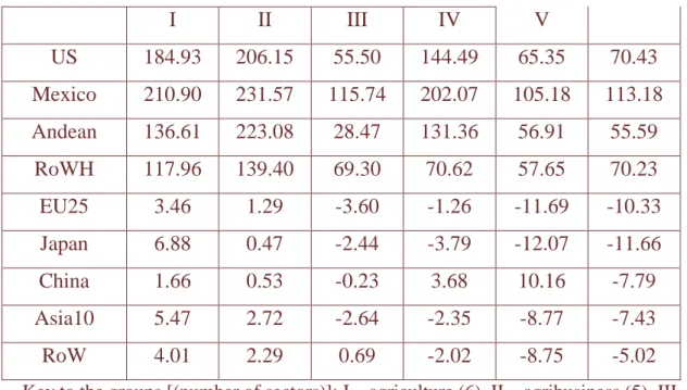
Table 8: Total trade flows changes (long run results), by Regions, for the four

Western Hemisphere scenarios.

EXPORTS IMPORTS

Scenarios Scenarios

REGIONS

A C D E A C D E

US 39.70 -1.06 -1.10 36.75 69.26 0.54 1.19 70.43

Mexico 5.55 119.58 -1.08 124.65 -8.42 138.96 0.83 113.18

Andean 3.46 -0.81 78.64 61.54 -3.16 0.66 55.33 55.59

RoWH 2.48 -0.72 -0.92 38.03 -5.69 0.65 0.87 70.23

EU25 2.12 -1.24 -1.77 -0.53 -10.76 0.19 1.07 -10.33

Japan 2.69 -1.67 -2.21 0.34 -11.70 -0.12 0.97 -11.66

China 2.09 -1.26 -1.93 -0.66 -8.77 0.57 1.07 -7.79

Asia10 2.27 -1.52 -2.32 -0.88 -8.08 0.26 1.00 -7.43

RoW 2.16 -1.09 -1.97 -0.67 -6.16 0.42 0.60 -5.02

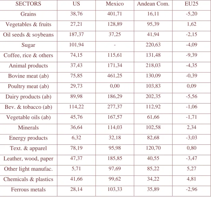
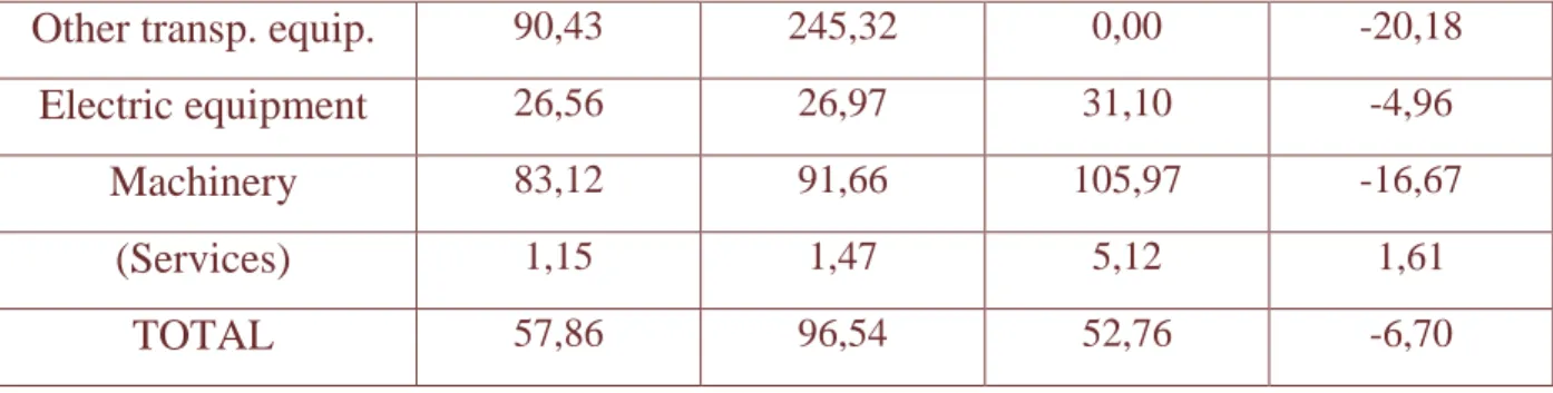
The additional insight provided by Table 9 refers to the market losses

(30)

comparison with Table 5 shows they usually lose market share, especially in the

case of the nine manufactures, either light or heavy, sectors; indeed, with the

exceptions of textiles & apparel (actually an increase) and non-ferrous metals

(nearly constant), the losses are significant. Similarly, for EU25 imports, the

table shows a uniformly greater market loss in all manufactures sectors, with the

exception of ferrous metals.

Table 9: The FTAA: Total trade flows changes (long run results; exports and

imports), by the four main regions, under scenario E.

9A. Exports.

Grains 38,76 401,71 16,11 -5,20

Vegetables & fruits 27,21 128,89 95,39 1,62

Oil seeds & soybeans 187,37 37,25 41,94 -2,15

Sugar 101,94 - 220,63 -4,09

Coffee, rice & others 74,15 115,61 131,48 -9,39

Animal products 37,43 171,34 218,03 -4,35

Bovine meat (ab) 75,85 461,25 130,09 -0,39

Poultry meat (ab) 29,73 0,00 103,83 0,09

Dairy products (ab) 89,98 186,29 202,35 -5,56

Bev. & tobacco (ab) 114,22 277,37 112,92 -1,06

Vegetable oils (ab) 45,76 167,57 61,66 -1,71

Minerals 36,64 114,03 102,58 2,34

Energy products 6,32 32,18 82,68 -3,03

Text. & apparel 78,19 95,98 120,70 0,80

Leather, wood, paper 47,37 185,85 40,55 -3,47

Other light manufac. 5,71 97,69 85,22 5,27

Chemicals & plastics 41,66 99,62 34,22 4,81

(31)

Non-ferrous metals 23,26 114,72 45,06 5,11

Motor vehicles 45,49 102,22 66,02 6,81

Other transp. equip. 32,40 361,28 98,09 2,30

Electric equipment 24,25 158,49 15,53 6,82

Machinery 18,08 169,35 37,84 13,05

(Services) -0,89 -1,07 -5,28 -1,36

TOTAL 32,47 118,11 60,14 -0,70

9B. Imports.

Grains 120,10 301,14 6,22

Vegetables & fruits 118,52 134,33 81,99 -6,07

Oil seeds & soybeans 137,37 162,12 224,22 4,23

Sugar

Coffee, rice & others 183,96 225,30 121,76 10,44

Animal products 193,44 220,28 177,15 3,36

Bovine meat (ab) 107,64 0,00 0,00 0,91

Poultry meat (ab) 87,14 0,00 76,94 -1,22

Bev. & tobacco (ab) 195,97 220,68 197,72 0,14

Vegetable oils (ab) 251,80 308,65 275,00 2,90

Minerals 109,75 115,74 87,37 -4,55

Energy products 28,69 20,45 0,94

Text. & apparel 211,24 227,52 184,53 -2,13

Leather, wood, paper 64,87 71,60 57,16 0,36

Other light manufac. 368,88 422,67 331,51 -7,64

Chemicals & plastics 40,51 43,48 38,08 -6,01

Ferrous metals 85,01 96,95 74,40 0,74

Non-ferrous metals 71,03 76,69 57,29 -6,08

(32)

Other transp. equip. 90,43 245,32 0,00 -20,18

Electric equipment 26,56 26,97 31,10 -4,96

Machinery 83,12 91,66 105,97 -16,67

(Services) 1,15 1,47 5,12 1,61

TOTAL 57,86 96,54 52,76 -6,70

The flows analysis is completed by looking at the Mercosul-China FTA.

Table 10 displays the regional changes it induces, by sector groups, while Table

11 gives a more detailed information on the total and Chinese flows.

Comparing Table 10 with Table 3, we see that, qualitatively, the

Mercosul-China FTA induces a pattern similar to the one generated by the

Mercosul-EU25 FTA. The difference, in exports, lies in group V, where

Mercosul exports now suffer a deviation in Asian and RoW regions, being not

affected in the remaining of the globe. In the case of imports, all regions, as

regards group IV, are now affected; deviations in group V are, however, more

modest.

Table 10: The Mercosul-China FTA (Scenario F): Trade flows changes (long run

results) by Regions and Groups of Sectors.

10A. Exports.

Sector Groups Total

Regions

I II III IV V

US -1.43 -1.06 -0.19 -0.83 0.93 0.18

Mexico -1.49 -0.54 -0.10 -0.53 1.57 1.06

Andean -1.09 -0.60 -0.54 -0.01 0.40 0.02

RoWH -1.21 -0.72 -0.26 -0.56 0.22 -0.27

EU25 -1.75 -0.66 -0.81 -1.64 0.20 -0.94

(33)

China 31.20 117.26 10.29 311.57 490.03 141.13

Asia10 -1.54 -0.85 -0.75 -1.90 -1.30 -1.29

RoW -1.71 -0.73 -0.97 -1.49 -0.05 -1.02

10B. Imports.

Sector Groups Total

Regions

I II III IV V

US 2.32 1.35 0.44 -2.75 -0.86 -0.84

Mexico 1.81 1.45 -0.05 -2.75 -1.41 -1.34

Andean 1.31 1.15 0.63 -2.03 -0.15 -0.37

RoWH 1.29 1.48 0.22 -0.44 -0.49 -0.14

EU25 2.28 1.39 0.20 -2.29 -1.51 -1.40

Japan 3.95 1.43 0.06 -7.40 -1.97 -2.01

China 196.71 339.17 35.77 286.55 103.92 142.74

Asia10 3.35 0.99 0.05 -3.21 -1.18 -1.40

RoW 2.66 1.47 0.73 -2.50 -0.76 -0.27

Table 11 shows that, in general, though the figures for the China flows are

usually high to very high, the impact in the total flows is small. Even so, it is

funny to see that many indications of contraction appear for total exports.

Definitely, China is an interesting partner whose role will evolve.

Table 11: The Mercosul-China FTA: Total and Chinese trade flows changes

(long run results; exports and imports) under scenario F.

Total flows Mercosul-China flows

Sectors

Grains

-0,46 0,63 10,46 -

Vegetables & fruits

(34)

Oil seeds & soybeans

-0,05 1,73 0,40 88,76

Sugar

3,23 8,80 427,89 -

Coffee, rice & others

3,61 6,09 264,23 140,81

Animal products

2,29 0,63 308,42 229,70

Bovine meat (ab)

-0,67 1,39 514,65 0,00

Poultry meat (ab)

-0,94 1,41 122,58 0,00

Dairy products (ab)

-0,82 1,61 0,00 0,00

Bev. & tobacco (ab)

-0,84 1,58 192,63 339,17

Vegetable oils (ab)

-0,18 0,91 95,92 0,00

Minerals

0,72 5,73 9,99 130,07

Energy products

-0,26 1,08 17,68 7,91

Text. & apparel

83,24 42,45 863,32 281,98

Leather, wood, paper

4,73 5,80 129,30 72,66

Other light manufac.

9,92 148,71 970,99 419,25

Chemicals & plastics

2,20 2,00 158,52 52,93

Ferrous metals

1,10 3,94 87,85 100,15

Non-ferrous metals

0,28 4,54 165,61 95,67

Motor vehicles

43,81 -3,47 1.551,86 462,18

Other transp. equip.

3,05 12,58 110,77 411,27

Electric equipment

3,27 1,62 233,41 35,33

Machinery

6,19 4,50 218,07 156,30

(Services) -1,12 1,40 -1,64 1,62

TOTAL 5,04 4,84 133,09 131,12

Correlation between the two patterns: i) Exports, 0.62 (without motor vehicles), 0.69 (with motor vehicles); ii) Imports, 0.46 .

Changes in trade flows have no clear, unidirectional relation with what

happens to output and, most importantly, welfare – the ultimate goal of any CGE

evaluation. Synthetic information on all the scenarios is obtained from Tables 12

(35)

Reminding that labour is reallocated in each scenario, keeping its total constant,

the two first tables show that, in general, changes induced by the six scenarios

are not very drastic. As expected, the directions of change are the same, in both

tables.

The Mercosul-EU25 agreement induces a more worrying contraction on

the heavy manufacturing sectors motor vehicles, other transport equipment and

machinery, what, for the two last ones, also happens with the US or FTAA

agreements, though with less intensity. This might be due to the impact of the

major unleashing of agribusiness exports to the EU, what might be distorting

somewhat the results. Moreover, given the more traditional sides of the European

economy, maybe there is less scope for Mercosul manufactures in that market.

The FTAA reduces output in the other light manufactures, chemicals &

plastics, non-ferrous metals and, especially, in other transport equipment and machinery sectors. The most notable increase takes place in motor vehicles. Part

of these results goes against those obtained in Flôres (2003) for Brazil, where the

FTAA slightly decreased ‘cars’ output (-0.4), while increasing ‘other vehicles’

(+2.1). Beyond the aggregation level (Brazil x Mercosul), the different base years

(1997, in Flôres (2003)) must be at play here.

Table 12: Total labour changes (long run results; percentage from base values),

for all scenarios.

Scenarios

SECTORS

Base

Labour* A B C D E F

Wheat, Corn and Other Grains 1.045,0 0,26 4,41 0,01 0,88 0,66 -0,22

Vegetables and Fruits 745,0 0,54 3,08 -0,12 -0,52 -0,81 -0,28

Oil seeds and Soybeans 1.350,0 0,52 2,08 -0,15 0,09 0,47 -0,20

Sugar 695,1 3,33 3,66 -0,40 -0,32 3,97 1,51

Coffee, Rice and Other Crops 1.228,2 1,13 5,51 0,03 -0,04 1,02 0,49

Animal Products 5.788,4 0,19 4,51 -0,03 0,21 0,44 0,05

Bovine Meat 425,0 0,71 24,87 0,09 -0,13 1,83 -0,02

(36)

Dairy Products 509,6 0,45 -0,86 2,68 1,40 4,52 0,05

Beverages and Tobaccos 506,0 0,43 -4,39 0,13 0,05 0,13 -0,04

Vegetable Oils 323,1 0,69 24,14 -0,59 1,26 1,87 -0,35

Minerals 1.131,0 0,39 0,77 -0,09 -0,21 -0,22 -0,18

Energy Products 366,0 0,56 0,10 -0,36 -1,03 1,05 -0,46

Textiles and Apparel 965,0 1,16 0,04 -0,26 0,75 1,51 2,78

Leather, Wood and Paper 2.321,4 5,70 4,96 0,66 -0,35 5,95 0,82

Other Light Manufactures 791,0 -3,21 -4,82 -0,06 0,12 -3,50 -11,84

Chemical and Plastic Products 1.885,0 -2,46 -4,22 -0,20 0,31 -2,33 -0,21

Ferrous metals 387,0 4,74 -1,44 1,03 0,49 6,44 1,28

Non-ferrous Metals 1.057,5 -1,40 -3,19 0,19 -0,39 -2,56 -0,06

Motor Vehicles 625,8 1,62 -15,06 2,50 2,81 8,11 13,09

Other Transport Equipment 645,8 -3,89 -13,83 0,01 0,20 -4,27 2,70

Electric Equipment 304,4 2,96 1,63 1,58 0,39 5,15 0,43

Machinery 1.354,1 -8,76 -10,12 0,78 1,17 -6,99 -1,79

Utilities and Construction 4.773,7 -2,75 -0,81 0,45 0,80 -1,64 0,48

Trade and Services 61.106,0 0,16 -0,43 -0,12 -0,16 -0,10 -0,10

Total 90.470,9 0,00 0,00 0,00 0,00 0,00 0,00

* in 1.000 workers

Table 13: Total output changes (long run results; percentage from base values),

for all scenarios.

Scenarios

SECTORS

Base

Values* A B C D E F

Grains 7,9 0,11 2,50 0,01 0,57 0,34 -0,13

Vegetables and Fruits 5,3 0,28 1,65 -0,08 -0,31 -0,60 -0,17

Oilseeds & Soybeans 12,5 0,24 0,90 -0,08 0,06 0,18 -0,10

Sugar 9,6 1,54 1,28 -0,20 -0,13 1,79 0,78

Coffee, Rice & Others 12,4 0,47 2,19 0,02 -0,01 0,40 0,23

Animal Products 63,6 0,08 2,12 -0,01 0,11 0,20 0,03

Bovine Meat 16,8 0,61 20,63 0,08 -0,11 1,54 -0,01

Poultry Meat 7,0 1,67 23,06 -0,32 -0,77 3,48 -0,39

Dairy Products 16,3 0,10 -0,88 1,28 0,70 1,97 0,04

(37)

Vegetable Oils 15,1 0,26 8,56 -0,22 0,47 0,70 -0,13

Minerals 25,8 0,21 0,39 -0,05 -0,12 -0,15 -0,10

Energy Products 35,5 -0,03 -1,60 -0,22 -0,55 0,07 -0,23

Textiles & Apparel 26,2 0,64 0,02 -0,14 0,41 0,82 1,52

Leather, Wood, Paper 45,2 3,81 3,31 0,44 -0,24 3,97 0,55

Other Light Manufac. 15,8 -1,80 -2,71 -0,03 0,07 -1,96 -6,74

Chemical & Plastics 60,0 -1,14 -1,96 -0,09 0,14 -1,08 -0,10

Ferrous metals 20,8 2,32 -0,71 0,51 0,24 3,15 0,63

Non-ferrous Metals 27,0 -0,92 -2,11 0,12 -0,25 -1,68 -0,04

Motor Vehicles 23,6 0,60 -16,34 1,59 2,37 5,62 11,14

Other Transp. Equip. 15,7 -4,37 -13,81 0,01 0,19 -4,77 2,58

Electric Equipment 13,6 1,08 0,60 0,58 0,14 1,87 0,16

Machinery 31,0 -4,56 -5,28 0,40 0,60 -3,63 -0,92

Utilities & Construction 124,2 -0,85 -0,25 0,14 0,24 -0,51 0,15

Trade and Services 641,9 0,10 -0,27 -0,07 -0,10 -0,06 -0,06

Total 1286,0 -0,03 -0,21 0,15 0,15 0,09 0,17

* in bn US$

Judging from a single figure of merit, Table 14 easily ranks the options.

Irrespectively whether GDP or EV is used, the competing pairs of scenarios are

B versus E and A versus F. The latter means that China, if on one hand inducing,

via its FTA with Mercosul, a trade flows pattern similar to that created by the

EU25-Mercosul FTA, on the other hand, in welfare gains, is already competing

with a US-Mercosul FTA.

Welfare results – both in plain real GDP variation, or in the more

sophisticated equivalent variation (EV) computation – are however surprisingly

low, for a model including imperfect competition. The explanation probably lies

on the fact that most gains, in all agreements, derive from the perfect competition

sectors, those in strategic interaction many times suffering a contraction. This is

(38)

Table 14: A few figures of merit: Total variations (long run results; percentage

from base values (in US$ bn)), for all scenarios.

Scenarios Base

Values A B C D E F

Real GDP 438,1 0,189 0,788 0,163 0,164 0,647 0.298

Welfare (EV) 75,7 0,377 0,482 0,082 0,056 0,630 0.257

Exports * 72,8 11,09 23,52 3,09 2,82 19,41 6,18

Imports * 68,5 12,31 23,40 2,77 2,34 19,86 5,93

* only merchandise trade

5. Mercosul: opportunities and defficiencies.

The fact of simultaneously analysing several integration possibilities provides

additional insights on the performance of the “invariant” partner, namely

Mercosul. In particular, questions of efficiency and adjustment may be identified

in a more consistent way.

It is tempting to divide the respective results in Tables 13 and 12, in order

to evaluate the variations in gross labour productivity, by sector, for each

agreement; this however is not very informative in the present exercise. The

constant total labour closure enhances the absolute value of the changes in this

factor, which, as mentioned above, have the same directions as those for output.

This implies that, uniformly, productivity decreases for a sector where output

expands, and increases for those that suffer a contraction. Though this can make

sense, the fact that it is a consequence of the mechanics of the model makes the

productivity analysis less realistic.

The issue of adjustment, called upon in a CGE context by Giordano and

Watanuki (2001) and Flôres (2003), remains a major one, especially for a bloc

with mixed characteristics like Mercosul. Based on Table 12, we derived a

classification of winning (W), neutral (N), conflicting (C) and losing (L) sectors.

Neglecting variations less than 1 per cent in absolute value, a sector is defined as

(39)

neutral, if no variations outside the 1 per cent range take place;

conflicting, if positive and negative variations appear outside the range;

losing, if all other output variations are negative.

Table 15 shows the result of directly applying the above criteria to data in

Table 12. The outcome is informative.

In the worldly competitive groups of Agriculture and Agribusiness, one

loser appears, beverages & tobacco, due to its contraction in the EU25 FTA. It is

worth pointing out that orange juice, a very performing Brazilian export is

subsumed in this sector. Also, oilseeds and soybeans turns out as a neutral sector.

In the Light Manufactures group the situation is not very encouraging, but

for leather, wood, paper where a basket of goods from Argentina, Brazil and

Uruguay have established market niches, with growth potential. Textiles &

apparel manages to be a winner, thanks to China, but other light manufactures is

a total loser. Things get worse in Heavy Manufactures. Three losers – including

the non-ferrous metals industry, what is both surprising and worrying – and two

conflicting cases are found. Out of the latter, the first is more of a winner, but for

the strong contraction in the EU25 scenario, and the second more of a loser, if the

increase in the China FTA didn’t take place. It is worth reminding that the

competitive Brazilian middle-sized aircraft are included in this last sector.

Finally, the pattern in the Energy group is faithful to Mercosul’s relatively

neutral standing in the two aggregate sectors.

It is also important to highlight that, out of the 13 winning sectors, 5 own

their classification to only one FTA result: all are in the Agriculture and

Agribusiness groups, and the FTA is the one with the EU25 which, as mentioned

in section 4, presents perhaps the more distorted – though not uninteresting -

result, driven by the opening of the CAP-protected market.

Table 15: A ‘Winners and Losers’pattern derived from the total output changes

in Table 12.

(40)

or Loser A B C D E F

Grains W - 2,50 - - - -

Vegetables and Fruits W - 1,65 - - - -

Oilseeds & Soybeans N - - - -

Sugar W 1,54 1,28 - - 1,79 -

Coffee, Rice & Others W - 2,19 - - - -

Animal Products W - 2,12 - - - -

Bovine Meat W - 20,63 - - 1,54 -

Poultry Meat W 1,67 23,06 - - 3,48 -

Dairy Products W - - 1,28 - 1,97 -

Bever. And Tobaccos L - -4,28 - - - -

Vegetable Oils W - 8,56 - - - -

Minerals N - - - -

Energy Products L - -1,60 - - - -

Textiles & Apparel W - - - 1,52

Leather, Wood, Paper W 3,81 3,31 - - 3,97 -

Other Light Manufac. L -1,80 -2,71 - - -1,96 -6,74

Chemical & Plastics L -1,14 -1,96 - - -1,08 -

Ferrous metals W 2,32 - - - 3,15 -

Non-ferrous Metals L - -2,11 - - -1,68 -

Motor Vehicles C - -16,34 1,59 2,37 5,62 11,14

Other Transp. Equip. C -4,37 -13,81 - - -4,77 2,58

Electric Equipment W 1,08 - - - 1,87 -

Machinery L -4,56 -5,28 - - -3,63 -

Summing up the previous analysis, a more nuanced interpretation of Table

15 can be provided:

Mercosul is clearly competitive in the following sectors: sugar; bovine and

poultry meat; dairy products; leather, wood, paper; ferrous metals; electric equipment and motor vehicles; the last one presenting problems in a EU25 FTA;

Mercosul clearly has competitiveness problems in the following sectors: other

(41)

For the remaining 10 sectors the bloc is roughly neutral, presenting sometimes

some competitiveness – 6 sectors – or more of a loser character – 2 sectors; only

2 remaining sectors qualifying as “true neutrals”.

Despite the proviso that the aggregation level of the sectoral division blurs

a mix of positive and negative situations – some exemplified above -, and the

inevitably arbitrary character of our “classification”, the final synthesis looks

quite reasonable. It lays bare a key defficiency of the bloc, which, unfortunately,

is really competitive in a few classical manufactures sectors and selected

segments of the agribusiness (plus sugar), i.e., lower value-added activities. All

non-competitive areas comprise key industrial sectors.

It is of course not necessarily bad for a bloc to have its trade assets in low

value-added sectors. Creativity and upgrading are important tools for improving

its terms of trade, as the Brazilian ‘sandálias havaianas’ and the Argentine

‘dulce de leche’-based goods show – beyond the persistent upgrading that

Mercosul meat exporters are accomplishing -, but clearly this is not enough. As

shown by a simple, aggregate CGE exercise, the bloc must seriously consider an

industrial adjustment process, to enhance its overall competitiveness and provide

it a better insertion in the world value-added chains. Whether this will be pursued

through a co-ordinated, internal political will, or forced, in a less planned (and

worse) way, via the route of FTAs, is a decision already in the realm of politics.

6. Conclusions.

Summing up the previous results, it seems that the imperfect competition sectors,

by keeping the segmented markets strategy, were able – in all scenarios - to

practice a kind of reciprocal dumping (à la Brander and Krugman (1983)), what

partially “saved” them from more drastic outcomes. Indeed, compared with a

carefully conducted study like Harrison et al. (2002), our corresponding results

are much less dramatic as regards output changes, decreases in these quantities