The effects of small firm tax incentives on employment levels

T

T

T

E

E

E

X

X

X

T

T

T

O

O

O

P

P

P

A

A

A

R

R

R

A

A

A

D

D

D

I

I

I

S

S

S

C

C

C

U

U

U

S

S

S

S

S

S

Ã

Ã

Ã

O

O

O

N

N

ú

ú

m

m

e

e

r

r

o

o

1

1

3

3

T

T

h

_h

e

_e

E

_E

f

_f

f

_f

e

_e

c

_c

t

_t

s

_s

o

_o

f

_f

S

_S

m

_m

a

_a

l

_l

l

_l

F

_F

i

_i

r

_r

m

_m

T

_T

a

_a

x

_x

I

I

n

n

c

c

e

e

n

n

t

t

i

i

v

v

e

e

s

s

o

o

n

n

E

E

m

m

p

p

l

l

o

o

y

y

m

m

e

e

n

n

t

t

L

L

e

e

v

v

e

e

l

l

s

s

Carlos Henrique L. Courseuil

IPEA ([email protected])

Rodrigo Leandro de Moura

IBRE and EPGE/FGV-RJ ([email protected])

2

The Effects of Small Firm Tax Incentives on

Employment Levels

1

Abstract

This paper aims to evaluate the impact on employment growth of a tax incentive program targeting Brazilian manufacturing small businesses (SIMPLES). This evaluation is conducted for two distinct periods: for the year 1997, when the program was first implemented, and for the year 1999, when the eligibility rule was modified to allow the eligibility of a broader group of firms. The evaluation takes into account two distinct channels through which the charted effects operate. The first is the employment variation in the firms that became eligible for the incentives, and the second is the change in the survival probability experienced by the same group of firms. Moreover, each of these channels can be activated either by the tax reduction dimension of the program or by its dimension of red tape simplification. Our results identify positive effects on employment growth for the tax incentive program only in the dimension of red tape simplification and its effects on the 1997 sample.

Keywords: employment, tax incentives. JEL Code: J21, H25.

1

3

1. Introduction

This paper will examine the effects of tax incentives on the employment level of small businesses. To achieve this, we will study the small business tax incentives program implemented in Brazil in the 1990s. The program, called SIMPLES, combines, simplifies and promotes the collection of federal taxes from micro-firms and small companies, introducing lower, though progressive, tax rates on the same base for calculation (gross revenues). The program aims to improve the performance of the target establishments, particularly with a view to move these establishments away from informality and toward boosting their employment levels.

Although frequently discussed among policymakers (see, for example, the World Bank [2009]), the question of the use of tax incentives to boost firms’ performance has not enjoyed similar support among academics. Existing studies focus on the impact of (fiscal incentive) programs on investment (Hasset and Hubbard [2002]; De Mooij and Ederveen [2003]; Klemm and Van Parys [2009]), leaving the question of the effect on employment open for discussion.

Another question frequently discussed among policymakers is the role of the small business in job creation. It is often said that this sector has a prominent role to play in employment generation and should therefore be the focus of incentive policies2. There is a good deal of discussion about this issue among academic economists,3 but little has been done to examine the possible impact of fiscal incentives on small businesses job creation4.

Our study makes a contribution, therefore, by casting light on a relevant question for public policies: do small businesses respond to tax incentives by changing their employment levels?

Note that SIMPLES combines reductions both in the monetary and administrative costs of tax payment. Therefore, another contribution of our study consists of its efforts to identify the effects of each of these mechanisms of the SIMPLES tax incentives. These mechanisms seem to be particularly important in Brazil, given that the World Bank (2010) ranks the country in the 152nd position among 183 countries for ease of paying taxes and in the 168th position for total tax rate5.

Our work also offers several methodological contributions. The main contribution occurs in the empirical part of the paper, where we were unable to use conventional methods to estimate the desired effect due to selection problems both in the treatment group and in the data sample. We overcome both of these problems by combining estimation procedures in alternative sub-samples.

While the principal contribution of this paper may lie in its empirical concerns, we also present a theoretical framework for the determination of employment at the firm level, and the effect of the introduction and extension of the SIMPLES program on firms’ employment level. This theoretical analysis is important because it identifies two different components of the effect of tax incentives on employment. The first incentive involves the changes in employment (due to the benefits of the program) for firms that would survive even if the program had not been implemented. The second deals with an eventual change in the size composition of the treated firms

2

See, for instance, Barack Obama and Joe Biden's Plan for Small Business available at www.barackobama.com/pdf/SmallBusinessFINAL.pdf.

3

On the one hand, Birch (1987) and Newmark, Wall and Zhang (2011) find evidence supporting the importance of small firms in job creation. On the other hand, Davis, Haltiwanger and Schuh (1996) present evidence that contradicts that presented by the above authors. Finally, Moscarini and Postel-Vinay (2009) show that the relative importance of small firms in the generation of employment varies according to the phase of the business cycle.

4

Lopez-Acevedo and Tinajero (2010) evaluate many programs oriented towards small business in Mexico, but none of these is similar to the SIMPLES program.

5

4

that derives from changes in the survival probability of these firms as they begin to experience the benefits of the program.

In the empirical aspect of the text, we use longitudinal data from Brazilian manufacturing firms to examine the contribution of the SIMPLES program to the average number of workers employed in those firm. The same empirical exercises are conducted at two distinct points in time: in 1997, the year it was implemented; and again in 1999, when there was an increase in the revenue threshold that determines the firm's eligibility for the program. Our strategy for identifying the effect of the SIMPLES program on employment decisions by firm is based on a comparison between the firms closest to the revenue threshold. In a broad sense, the rationale for doing this is to contrast the employment level of those firms that opt for the program relative to the level of those that do not opt for the program. Our challenge was to identify each component of the effect in the presence of both selection problems, that of the treatment group and that of the data sample.

Finally, we would like to point out that, in addition to the level of employment in existing firms and their survival probability, another relevant dimension for job creation is represented by the entry of new firms. This issue is not addressed in this article. The studies by Monteiro and Assunção (2009), and Fajnzylber, Maloney and Rojas (2011) offer a useful discussion of this topic, and can be seen as complementary to the present paper6.

The remainder of the article is structured in the following manner: The second section presents the theoretical framework. The third section outlines our strategies for the identification and estimation of each of the effects mentioned above. The fourth and fifth sections are dedicated to the presentation and discussion of the database and the empirical results, respectively. The last section presents a brief summary and some conclusions.

2. Theoretical Framework

In this section, we describe our view of how companies make decisions regarding labor demand. We propose a simple theoretical framework in which firm dynamics is driven by the evolution of the firm’s idiosyncratic productivity component. This is in line with the literature on firm size distribution, except that we incorporate taxation in two distinct regimes: the standard and the simplified (the latter resembling the tax structure of SIMPLES). After a brief discussion of the theory, we develop some predictions of how the SIMPLES incentives will affect decisions about labor demand.

2.1. Assumptions

The context consists of an economy with firms producing homogeneous goods in a competitive

market, using labor ( _t) as the only input. The current profits of the firms can be described by the

following equation:

, . ) ( . . ). 1

( _{t t t t t t}

t = −

τ

p u f −w

π

₍₁₎

where p_t and w_t corresponds to price and wage respectively and

τ

_t is a revenue tax that varies according to the tax system, τt =

{ }

τs,τn . The first value corresponds to the tax rate that applies

6

5

when the firm opts to enroll in the SIMPLES program, and the second value corresponds to the standard tax rate7.

As with other calculations of firm dynamics, profits are affected by the term u_t, which

represents firms' idiosyncratic productivity component, or (as we will refer to it) the efficiency level. The main hypothesis of the model refers to the evolution of this term over time, which is formalized below:    + = = + + = − − − otherwise v u and if v k u u t t s t n t t t t , , 1 1

1 τ τ τ τ

, (2)

where v_t represents white noise. This shows that the process driving the evolution of the firm's efficiency is a random walk with drift when the firm migrates from the standard tax system to the simplified one and is a pure random walk in all other situations. The drift component (represented by k) is motivated by the lessened requirements for red tape procedures (achieved by the simplification of tax forms and filing) in SIMPLES.

Given the absence of costs of adjustment or of any other factor that would make the choice of employment level an inter-temporal decision, the firm decides to maximize the expected value of current profits. Once we assume that pt and wt are known at the beginning of period

t

8 , then

t

u becomes the key ingredient on employment decision. Based on the assumptions of a random

walk process for ut, one can easily deduce the following:

   _{+ = =} = − − − − − otherwise u and if k u u u E t s t n t t t t t t , , ] , , | [ 1 1 1 1 1 τ τ τ τ τ τ (3)

In fact, in the empirical aspect of the paper, no firm is eligible for the SIMPLES program in 1

−

t , which allows us to condition the expectation only in terms of u_t−1 and

τ

_t.

For convenience, we will assume a specific form for the production function as specified by ).

1 ln( )

( _t = _t +

f

Hence, the firm chooses its employment level by maximizing the following definition of expected profits:

(

t

)

t t t t t t t t

t p E u u w

E t t . ) 1 ln( ]. , , | [ . 1 max ] [

max π = −τ −1 τ τ −1 + −

The optimal level of employment is given by:

( ) ( )     = − = − = − − − + − ∗ n t w u p s t w k u p t if if t t t n t t t s τ τ τ τ τ τ , 1 , 1 1 1 1 ) ( 1 (4) 7

We are abstracting from the fact that the standard tax system is more complex, combining revenue tax with VAT and payroll taxes.

8

6

Let T be a binary variable that shows whether the firm opts to enroll in the SIMPLES program. The relationship of this variable to the optimum employment level can be seen in its clearest form by reconfiguring the equation above as follows:

(

)

(

)

( )

_k

w p T u w p T u w p t t s t t t s n t t t ns t . 1 . . . 1 . 1 1 1

τ

τ

τ

τ

_{− +} − ₊ −

−

= _{− −}

∗

(5)

The equation above reveals an important property of our model: the identification of both dimensions of SIMPLES benefits. The reduction in tax rates drives the first term that is multiplied by T , while efficiency gains due to reduction in red tape procedures drive the last term.

Concerning the choice of tax system, it is obvious that all eligible firms will prefer the simplified scheme. Therefore we may write the following definition for τ_t:

   > + < + = − − − − − − c u p if c u p if t t t n t t t s t ) 1 ln( . . , ) 1 ln( . . , 1 1 1 1 1 1 τ τ τ (6)

Another important decision to be made by the firm is whether it should continue to operate. At the start of each period, the firm decides to shut down (forever) or to continue operating for another period. Note that this decision is inter-temporal in its nature, given that what is decided in period t will have an impact on decisions to be made in t+1. To simplify this decision, it is assumed that the firm is aware of the entire trajectory of price and wage levels.

In the Appendix, we derive the following result:

1) For each (

τ

), there is an lower bound of u_t−1 that determines the permanence of the firm. We call this limit γ′

( )

τ . When u_t−1 is found to be below this level, the firm decides to cease its activities; otherwise, it remains in the market.

Hence, we can interpret ∗t as a latent variable and define the optimal level of employment as:

( )

( )

   ′ ≤ ′ > = − − ∗ τ γ τ γ 1 1 , 0 , t t t obs t u u (7)

2.2. Predictions about the Effects of SIMPLES

The equation (5) allows us to examine the effect of the SIMPLES program on latent employment ( ∗). Because (τns −τs) _{is positive, like all the other terms pre-multiplied by T , it}

follows that:

The optimal latent employment level increases (equation 5) when the tax rate is reduced from τn

to

s

τ (which is to say when T changes from 0 to 1), all else remaining constant.

The identification of this effect of SIMPLES in a particular subpopulation of firms is our main goal. To be precise, we define our main parameter of interest as:

)] ( ; , | [ )] ( ; , |

[ 1 1 1 1

n t t n n t t s u u E u u

E

τ

γ

τ

τ

γ

τ

α

′ − − ∗ ′ − −

∗ _{> − >}

= ₍₈₎

7

change if firms that would have survived even if the program had not been implemented get the treatment? There are two comments to be made about this parameter. First, this corresponds to an ATNT (average treatment effect on non-treated population) parameter. Second, the effect captured by this parameter varies with u_t−1, as can be immediately derived from equation 5.

The identification of this parameter is not a simple task. Sample selection concerns should be taken into account since this survival decision is also affected by changes in tax rates. In the Appendix, we prove the following prediction:

2) The lower bound for u_t−1 (at which point the firm decides to shut down), γ′(τ), diminishes when the tax rate is reduced from τn

to τs

and all other factors remain constant. In other words, γ′(τs)<γ′(τn)_.

A third prediction emerges naturally as a corollary to the prediction above: 3) Some firms that decide to leave the market when subject to tax τn

decide to stay if they are instead subject to tax rate τs

. These firms are those for which ( ) t ₁ ( n)

s

u

γ

τ

τ

γ

′ < ₋ < ′ . Another corollary also follows from this one:

4) The firms that close down their activities when subject to tax rate τn_{, but do not close when}

subject to tax rate τs

, tend to be smaller than those that survive when subject to either one of the two tax rates.

The corollary above is based on the fact that ∗t is directly proportional to ut−1, as shown in

equation (4). As a result, the mortality rates of firms that opt for the SIMPLES program may change as well; in particular, firm mortality tends to decrease among the smaller firms, changing the composition of the treated group with regard to firm size. The identification of

α

must refrain from including this sample selection (composition) effect as part of the measure of the effect of SIMPLES on firm level employment decisions. Our strategy for accomplishing this task is discussed in the next section.

3. Identification of the ATNT parameter

Our strategy for identifying the impact of SIMPLES described by

α

contains three steps. In a first step, we identify another parameter that we claim can be defined as the sum of

α

and a selection term. In the second step, we identify this selection term, and in the final step we reach the identification of

α

by subtracting these two objects. That is, we first identify the ATNT parameter with a bias term produced by sample selection (composition effect) and self-selection. We then identify the bias term, which can be removed due to the additive separability prevailing in the first step.

This indirect way of reaching the identification of

α

is necessary due to the fact that we need data for two consecutive years, as will become clear below; this means that at the very least, the sample selection cannot be ruled out straight away.

3.1. From the theory to the empirical model

Equation (5) can be rewritten in the following way: ,

. .

. .

1 ₁ t _{1 2} t t _{1 3} t

t =− +

δ

u +

δ

T u− +

δ

T

′ − ′ ∗

8

where

δ

_{combines variables that are constant across firms. To be precise, this relation takes the}

forms ( )

t t ns w p τ

δ′ ₌ 1−

1 , ( _t )

t s n w p τ τ

δ′ ₌ −

2 , ( )_t k

t s w p . 1 3 τ

δ ₌ −

. In these formulations,

δ

2′ is the parameter related

to the tax rate reduction and δ₃ is related to the rate of bureaucracy simplification.

Note that u_t−1 is not observable but can be retrieved from the definition of gross revenue

(R) represented by:

. ) ( . 1 1 1 1 − − − − = t t t t f p R u

Admittedly, other factors may influence a firm's employment level. Some of these may be captured by observable variables that will be denoted by X 9. Others will be aggregated in a non-observable, idiosyncratic component, which leads to our empirical model that is described as follows: , . . . .

. _{1 2 1 3}

1

0 t t t t t t

t =

δ

+

δ

µ

+

δ

T

µ

+

δ

T +X Ω+

ε

′ −

− ₍₁₀₎

where _{1 ( )}

1 1 − − = − t t f R t

µ and

1 − ′ = t k p k δ

δ for k∈

{ }

1;2 . ε_t captures the idiosyncratic factors mentioned above. We assume that it is an iid random variable (across firms and time) with zero mean whose value is revealed to the firm at the beginning of period t.

In considering the non-observable idiosyncratic component among the employment determinants, we also need to adapt the equation for survival decision (equation 7). Plugging equation 10 on 25 (See the proof in the Appendix, in the section dealing with the survival decision in the theoretical model), one can easily see that firm survival will be guided by a condition of the following type:

). ( ) ,

(u_t−1 ε_t >γ τ

h ₍₁₁₎

At this point, we are ready to discuss the identification and estimation of our parameter of interest based on the three steps mentioned above.

3.2. First Step: Identification of the Biased Effect

We argue that a trivial comparison identifies the sum of our main parameter,

α

, with a selection component,β, for specific values of µ_t−1. This comparison contrasts the average employment level in surviving and treated establishments with the average of those that also survived but were not treated, conditioned on particular values of the ratio revenue-production and also on the other observable variables denoted as X in equation 10. This corresponds to the following equation (proved in the Appendix in the section concerning identification of alpha and beta)10:

, )] ( ) , ( ; , 0 | [ )] ( ) , ( ; , 1 |

[ ∗ =

µ

_{−1 −1}

ε

>

γ

τ

− ∗ =

µ

_{−1 −1}

ε

>

γ

τ

n =

α

+

β

t t t t t s t t t t

t T h u E T h u

E ₍₁₂₎

where β represents the selection component mentioned above, which can be defined as follows using the share of firms that depend on the SIMPLES program for survival (ρ):

( )

_. )] ( ) , ( ; , 1 | [ )] ( ) , ( ; , 1 | [ . 1 1 1 1       > = − < < = = − − − − n t t t t t s t t n t t t u h T E u h T E τ γ ε µ ε τ γ ε τ γ µ ε ρ β (13)

The expression above contrasts the non-observable idiosyncratic component of those firms

9

We included dummy variables for industry groups in manufacturing, for states, for one-establishment firms and for age groups.

10

9

that need the program to survive with those that do not. The survival rule guarantees that the first group has no parallel among the non-treated firms, a distinction that generates a sample selection bias.

In addition, because we are dealing with the treated firms, an auto-selection bias may also be captured by the above parameter. This bias will occur if the association between the non-observable idiosyncratic component and the program participation likelihood differs between those firms that need the program to survive and those that do not. Possible reasons for the distinct participation likelihood across these two groups are heterogeneity either in the gains of participation or in the access to information regarding participation.

There is an alternative way, besides that of equation (13), to define β. Using equation 10, one can easily derive the following alternative definition of β:

( )

( )

_. )] ( ) , ( ; , 1 | [ ] ) , ( ; , 1 | [ . 1 1 1 1       > = − < < = = − − − − n t t t t s t t n t t u h T E u h T E τ γ ε µ τ γ ε τ γ µ ρ β (14)

Although not feasible as an identification strategy, this alternative definition for β is useful both for building a feasible strategy and for interpreting this selection term. As we stated in the theoretical section (prediction 4 in the section called Predictions about SIMPLES Effects), some firms continue operating when subject to the conditions of SIMPLES that would have ceased operations if there were no such program. These firms tend to be smaller than those that do not need the program to survive (prediction 5). The expression above shows that β captures the average size difference between these two groups of treated firms. Therefore, if the sample selection (i.e., the composition effect) is the driving force here, then β should have a negative sign.

3.3. Second Step: Identification of the Bias Term

We now turn to the second step of our procedure. For the sake of identification of the bias term, we must rely on at least two assumptions. Consider that the program was implemented in year t. The first assumption is that, at t−1, the (unobservable) idiosyncratic component is not related to the treatment status of the firm at t for a sub-sample that is able to survive up to t, even when subjected to the traditional tax system. These are the firms for which h(ut−₁,

ε

t)>

γ

(

τ

n). Therefore, we can state our first identification assumption as:

[

| 0, ; 0, ( , ) ( )

]

. )] ( ) , ( , 1 ; , 0 | [ 1 2 1 1 1 2 1 1 n t t t t t t n t t t t t t u h T T E u h T T E τ γ ε µ ε τ γ ε µ ε > = = = > = = − − − − − − − − (15)

The equation above may be interpreted as ruling out self-selection at t – 1 among the firms that do not need the program to survive. Note that we are ruling out self-selection before the program is implemented only for the group of firms that do not need the program to survive. Hence, the hypothesis above does not rule out that self-selection may be operating at the time the program is implemented (t) for any firm; for those firms that depend on the benefits of the program to survive, we consider that self-selection can take place even before implementation.

10

( )

( )

( )

( )

[

]

_. )] ( ) , ( , 1 ; , 0 | [ ) , ( , 1 ; , 0 | )] ( ) , ( ; , 1 | [ ] ) , ( ; , 1 | [ 1 2 1 1 1 2 1 1 1 1 1 1       > = = − < < = = =       > = − < < = − − − − − − − − − − − − n t t t t t t n t t s t t t t n t t t t t s t t n t t t u h T T E u h T T E u h T E u h T E

τ

γ

ε

µ

ε

τ

γ

ε

τ

γ

µ

ε

τ

γ

ε

µ

ε

τ

γ

ε

τ

γ

µ

ε

(16)

The two groups represented are those able to survive up to t because of the program and those that are able to survive without the program.

To interpret the equation above, note that, so far, the gap in the idiosyncratic component between the two groups of treated firms is driven by sample selection and possibly also by self-selection among those firms who depend on the program benefits to survive. In this setup, the equation above can be interpreted in the following manner. The same combined effect produced by these two sources should be operating both at the time the program is implemented (t) and the time period just before the program implementation (t−1), once we fix the sample for surviving firms.

Under these two assumptions, we prove in the Appendix (section Identification of bias term: Proof) that β can be identified by the following difference:

[

]

[

]

. ) ( ) , ( , 0 ; , 0 | ) ( ) , ( , 1 ; , 0 | 1 2 1 1 1 2 1 1       > = = − > = = − − − ∗ − − − − ∗ − n t t t t t t s t t t t t t u h T T E u h T T E τ γ ε µ τ γ ε µ (17)

This is the difference in employment level just before the introduction of the program between i) firms that had been treated in the following year and had survived until then, and ii) firms that had not been treated in the following year but had also survived until then. Conditioned on the proxy for the efficiency level (i.e., the ratio revenue-production), there is no reason, other than selectivity, to expect differences in the employment levels between these two groups.

We would like to stress two aspects of the equation above. First, the sample restriction to firms surviving one year after the decision period guarantees that the sample selection (composition) effect occurs. Second, the fact that we compare the firms in

( )

t−1 means that the treatment has no direct effect in their employment level because they are all subject to the same pre-program tax rate.

4. Identification of the composition effect

The identification strategy discussed above does not allow the isolation of the composition effect from the auto-selection component. The goal of this section is to propose two alternative strategies for the identification of the composition effect.

The first alternative is to make further assumptions in the same framework discussed above. The second alternative departs from the theoretical foundation used so far and explores the fuzzy discontinuity design of the program participation rule.

11

In the first alternative, we rule out self-selection from the bias component identified in the second step of the strategy described above. Remember that we have already assumed that self-selection was absent at t−1 among the surviving firms that do not need the program to survive. Now we assume that there is no association at all between the non-observable idiosyncratic component and the program participation likelihood at t. To be precise, we propose that the following relation holds true for a random sample of firms:

. 0 ] , , |

[ _t T_{t t−1} X_t =

E ε µ ₍₁₈₎

This means that once we condition for a given labor productivity level and for other observable factors, the non-observable idiosyncratic component of the firm is not related to its treatment status in a random sample of firms. This is to say that, if we pick at random one firm that opted for the SIMPLES taxation scheme and another that opted for the traditional one, these should not differ with respect to the non-observable idiosyncratic component when they have similar labor productivity levels and other observable factors.

One may question the plausibility of the above assumption based on the possibility that some of the firms with revenue just above the eligibility threshold could underreport it to get the benefits of the program. If this was the case, there could be an indirect correlation between ε_t and treatment status in the labor productivity level. However our information on revenue is based on firms' responses to a survey that is not used by the authorities for procedures related to the enforcement of any rule11. Therefore, there is no need for firms to underestimate their revenue, even when declaring themselves as treated units.

Another concern is that some firms may anticipate that their annual revenue will be just above the eligibility threshold and make adjustments that would not have be considered if the program were not implemented. Such adjustments could be implemented either by postponement part of firm sales for the following year or by hiding sales off the books. This may imply a similar correlation to the one mentioned above. However, the timing of the SIMPLES legislation helps us to assert that this practice should not be relevant. The threshold value of R$ 720,000 for 1996 gross revenue, which defined eligibility for 1997, was defined by law in December 1996 and was raised to R$ 1,200,000 by a law passed in December 199812. Therefore, we argue that in 1996 and 1998 firms could not manipulate their revenue flow to match the eligibility criteria because they would have learned about this criterion in the last month of the respective years.

It is easy to see that the biased effect of the previous strategy becomes the pure sample selection (composition) effect once we get rid of the self-selection component.

4.2. Fuzzy Regression Discontinuity Design (FRD)

Our second strategy for the identification of the composition effect explores the discontinuity in the eligibility rule of the program in a quasi-experimental context. In doing so (unlike what we did in

11

This is explicitly stated in the survey questionnaire.

12

12

the previous strategy), we refrain from using the structure imposed by the theoretical framework. In the remainder of this section, we show that such a strategy is able to identify a biased effect that corresponds to the sum of the scale effect and a pure sample selection term. Our intuition is that the FRD method eliminates self-selection.

The departure point of the present identification strategy is the following regression model, which has no direct connections with our theoretical model and should thus be viewed as a reduced form:

, )

( )

( 1 2 3 1 4

1

0 t t t t t t

t =λ +λ R− −c +λ T +λ D R− −c +λ X +ε (19)

where, T and D are dummies indicating the treatment status and eligibility for the SIMPLES program. X denotes other control variables as before, while c represents the eligibility threshold mentioned above.

In accordance with the FRD strategy, we use the eligibility variable (D) as an instrument for the treatment variable T . The effect that we can identify corresponds to the following:

[

] [

]

[

] [

]

[

] [

]

[

] [

]

, , | , | , | , | , | , | , | , | 2 1 1 1 1 2 1 1 1 1 ξ λ ε ε λ λ λ + = = − = = − = + = = = − = = − = = + − − − + − − − + − − − + − − − t t t t t t t t t t t t t t t t t t t t t t t t X c R T E X c R T E X c R E X c R E X c R T E X c R T E X c R E X c R E (20)

where the first term of last line (λ₂) corresponds to the ATNT parameter, and the last term captures the selection bias. Therefore, as with the previous strategy, in this first step we identify a biased effect. Also like the previous strategy, we claim that this bias is driven only by the sample selection and is not affected by self-selection.

The implicit identification hypothesis in the present strategy is the following:

( )

[

| ₋₁ = −, , ( ₋₁, )>

]

−

[

| ₋₁ = +, , ( ₋₁, )>

( )

n

]

=0.

t t t t t n t t t t

t R c X h u E R c X h u

E

ε

ε

γ

τ

ε

ε

γ

τ

₍₂₁₎

The same kind of decomposition used in the previous section can be replicated here to redefine ξ, which under the above-stated hypothesis becomes:

( )

( )

[

]

[

] [

]

( )

[

]

[

| ,

] [

| ,

]

. ) , ( , , | , | , | ) , ( , , | 1 1 1 1 1 1         − ⋅ = + − − − − − + − − − − − = − = > = = − = < < = t t t t t t n t t t t t t t t t t t n t t s t t t X c R T E X c R T E u h X c R E X c R T E X c R T E u h X c R E τ γ ε ε τ γ ε τ γ ε

ρ

ξ

(22)

Notably, unlike the previous strategy, we do not rule-out self-selection from the beginning of these considerations. Here, this source of bias is expurgated by the use of the IV method.

The estimation of the parameter

λ

(λFRD

) is conducted by instrumental variable, where the estimator corresponds to the sample analogue of the right-hand side term in the first line of (FRDlambda). As becomes evident in the second line of this same expression, the equation estimates the sum of the ATNT parameter and a sample selection term.

To disentangle these two components, we rely on our estimation for the ATNT parameter according to the previous strategy. Therefore, the sample selection term can be described as:

. ols FRD frd λ α

ξ = − ₍₂₃₎

13

The main source of data is the Pesquisa Industrial Annual (PIA), an annual longitudinal survey of manufacturing establishments conducted by IBGE (the Brazilian Census Bureau). We use the files for the period from 1996 to 1999. The data allows us to match information regarding employment, enrollment in the SIMPLES program and gross revenues, and all of the other variables mentioned in the specification of the empirical model13.

To offer some descriptive statistics about the variables that we use in the analysis of the SIMPLES program, Table 1 shows that, among the firms sampled in the PIA in 1997, 42,289 firms were eligible for the SIMPLES program and, of these, 32,735 (77.4%) decided to opt for the SIMPLES program for that year. In addition, we note that there are firms that would not have been eligible for the program according to the gross revenue requirement, but which have identified themselves as participants in the SIMPLES program. This apparent inconsistency in the data may reflect either error in the revenue declaration by firms or negligence with regard to other eligibility criteria. But the magnitude of these errors is small because only 734 firms fall into this group14,15.

This small number of firms shows that the 1996 revenue is, in fact, the most important criterion or that the others are not quite so relevant.

In 1999, there was a significant increase in the number of firms eligible for (and choosing to enroll in) the SIMPLES program16, to 59,128 eligible firms; of these, 48,425 (81.9%) were (auto-)selected into the program. In addition, the number of firms that would not be eligible for the program according to the gross revenue requirement, but which identified themselves as participants in the SIMPLES program, was reduced to a little more than 450 firms. So once more, gross revenue seems to be the unique criterion that effects eligibility. In Table 2, we can see the mean and standard deviation statistics calculated for several variables. In average terms, the firms had 68.8 workers in 1997 and 56.3 in 1999. Among firms that opted for the SIMPLES program, these figures decrease to around 15 workers in both years.

We should also note that the firms that opted for the SIMPLES program are younger than the ones that didn't and that the vast majority of the first group have only one establishment (98%).

Table 1: Frequency of Firms Opting for SIMPLES in 1997(9) by 1996(8) Revenue

13

The sample design of PIA for a given year is based on the following restrictions: (i) the establishment must have appeared in an administrative file (RAIS) that includes all formal (registered tax payers) establishments from the previous year and (ii) if it had between 5 and 30 employees in the file, it will have a random probability of being sampled into PIA, and if it had more than 30 employees, it will be automatically sampled; if it had less than 5 employees, it would automatically not be sampled.

Note that condition (i) implies that the PIA does not include firms in their first year of activity, which prevents us from (directly) estimating the impact of SIMPLES on the creation of new firms in any of our estimates. Condition (ii) is in turn a source of attrition, but this is exogenously driven, and thus won't affect the estimates of the SIMPLES effect.

14

This occurs because, according to the legislation, the gross revenue that is considered as a criterion for eligibility should deduct canceled sales and any granted unconditional discounts. For part of the sample we provide detailed information on these items. We performed a re-estimation of all the models by deducting these items from the gross revenue for this part of the sample. The results did not change.

15

There is another component of this measurement error that we were unable to observe: there were firms that would have been eligible but were classified as a non-eligible and did not opt for the SIMPLES program. However, because the majority of eligible firms opted for the SIMPLES program, this other source of measurement error probably is even more negligible, given that only 734 of the non-eligible firms opted for the SIMPLES program.

16

14

No (%) Yes (%) Total (%) Opting for SIMPLES

No 20,838 32.63 9,554 14.96 30,391 47.59 Yes 734 1.15 32,735 51.26 33,470 52.41 Total 21,572 33.78 42,289 66.22 63,861 100 Opting for SIMPLES

No 17,199 22.4 10,703 13.94 27,902 36.34 Yes 453 0.59 48,425 63.07 48,878 63.66 Total 17,652 22.99 59,128 77.01 76,780 100

Note: Based on Data from the PIA.

Eligible if 0<=gross revenue in1996<=720000 and Non-Eligible if gross revenue in 1996>720000 for 1997 Eligible if 0<=gross revenue in1998<=1200000 and Non-Eligible if gross revenue in 1998>1200000 for 1999

1999

15

Table 2: Statistics for Several Variables

Variable Mean Std Dev Mean Std Dev Mean Std Dev

Number of workers - 96 68.36 384.02 128.44 549.67 15.55 74.50

Number of workers - 97 68.86 383.28 128.72 547.92 15.68 68.40

Number of workers - 98 57.63 326.58 130.64 526.37 14.85 42.83

Number of workers - 99 56.31 321.22 130.14 524.89 14.90 41.67

Opting for SIMPLES - 97 0.53 0.50 - - -

-Opting for SIMPLES - 99 0.64 0.48 - - -

-Elegible - 97 0.66 0.47 0.30 0.46 0.98 0.15

Elegible - 99 0.77 0.42 0.38 0.48 0.99 0.10

One Estableshiment - 96 0.86 0.35 0.72 0.45 0.98 0.13

One Estableshiment - 97 0.87 0.33 0.74 0.44 0.98 0.12

One Estableshiment - 98 0.90 0.30 0.76 0.43 0.98 0.12

One Estableshiment - 99 0.90 0.30 0.74 0.44 0.98 0.12

Age - 96 13.37 9.55 16.87 10.98 10.29 6.73

Age - 97 14.56 9.65 18.11 11.07 11.40 6.75

Age - 98 13.38 9.58 18.17 11.44 10.57 6.89

Age - 99 14.46 9.65 19.57 11.46 11.59 6.98

Gross Revenue - 95 5,727,307 125,659,380 11,643,840 182,962,565 526,318 13,647,651

Gross Revenue - 96 6,576,364 124,276,696 13,349,555 180,108,528 558,463 16,383,215

Gross Revenue - 97 7,309,252 137,616,322 14,877,204 199,622,547 585,215 16,218,939

Gross Revenue - 98 6,064,905 120,793,210 16,279,496 200,779,871 334,970 8,425,016

Gross Revenue - 99 7,135,742 158,249,260 19,184,744 263,269,476 376,784 9,127,971

Number of Observations - 97

Number of Observations - 99

Note: Based on Data from PIA

16908 7356

Full Sample Opting for SIMPLES

No Yes

22656 17837 4819

24264

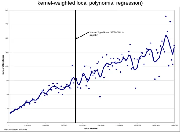
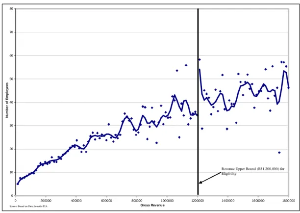
Finally, we will provide empirical reasons to use Fuzzy Regression Discontinuity Design (FRD) in a quasi-experimental context. Figures 1 and 2 in the Appendix attempt to answer the following question: Is there a discontinuity in the number of employees for firms with revenues around the revenue threshold? Initially, we found that firms with a higher level of income tended to have a larger number of employees, which we expected. However, it is important to point out that the firms that were eligible for the SIMPLES program (in other words, firms with revenue lower than the vertical solid line: below R$ 720,000 in 1996 and R$ 1,200,000 in 1998) show lower dispersion in terms of the number of employees then do the non-eligible firms. In addition, we estimated a kernel-weighted local polynomial regression17 (continuous line) that suggested that the impact on the employment level around the revenue upper bound is nil for 1997 and that this favored the non-eligible firms (those with income greater than R$ 1,200,000) in 1999. Nevertheless, it is notable that this impact is not controlled by the selection mechanisms (indicated above) nor by the other factors captured by the control variables.

17

16

6. Estimation Methods and Results

Section 4 provides two alternative identification strategies. Each alternative motivates a specific estimation procedure to be detailed in the present section.

Both strategies are defined in two steps. Also, in both cases the first step identifies what we call the biased effect, which consists on the sum of the ATNT and a bias parameter, while the second step disentangles these two components. The same steps will be followed in the respective estimation procedures.

6.1. First Estimation Procedure: OLS

The first step of the first strategy relies on a comparison of the employment level across treated and non-treated firms with similar observable characteristics, as indicated by equation (12). This suggests that the OLS estimator of equation 10 provides the first step of our first estimation procedure.

Note that the estimand has two components (δ₂.µ_t−1 and δ₃) that are associated through our theoretical framework with the tax rate discount and the red tape simplification components of the SIMPLES program, respectively. Moreover, the first of these components depends on µ; therefore, our estimation will be evaluated at the sample average value of this variable. The sum of these two components will provide our estimation for the biased effect (α+β).

Similarly, the second step of the first strategy relies on a comparison of the lagged employment level across treated and non-treated surviving firms with similar observable characteristics, as pointed by equation (17). This suggests that the OLS estimator in the following regression model provides the second step of our first estimation procedure:

, ~ . .

. .

. _{2 2 2 3 1 1}

1 0

1 −

′ − ′

− ′′ − ′′ ′′

− = + t + t t + t + t Ω+ t

t

δ

δ

µ

δ

T

µ

δ

T X

ξ

₍₂₄₎

which corresponds to the original model with all variables lagged as shown below: ,

~ .

. _{2 1 1}

1 0

1 −

′ − − ′′ ′′

− = + t + t Ω+ t

t

δ

δ

µ

X

ε

Note that we have decomposed ε_t−1 in a selectivity component (

δ

₂′′.T_t.

µ

_t−2+

δ

₃′.T_t) and another random one (ξ_t−1). The OLS estimation for 2

.

−2

′′

t

µ

δ

corresponds to our estimation for the

bias in the tax cut effect, while the corresponding estimation for

δ

₃′ will provide our estimation of the bias in the red tape simplification effect of the SIMPLES program. The sum of these two values will provide our estimation for the overall composition effect (β).

17

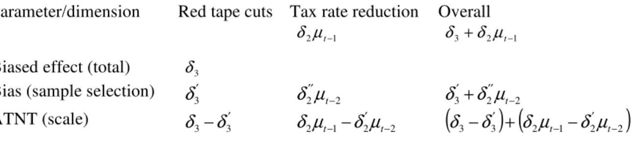
Table 3. Theoretical Parameters and Dimensions of the SIMPLES Program Effect

Parameter/dimension Red tape cuts Tax rate reduction Overall

Biased effect (total) δ3

1 2µt−

δ δ₃+δ₂µt₋₁

Bias (sample selection) ′ 3

δ

δ

₂′′

µ

t₋₂ 3 2 −2

′′

′₊

t

µ

δ

δ

ATNT (scale) ₋ ′

3 3

δ

δ

2 1 2 −2

′

− − t

t

δ

µ

µ

δ

(

3 3

) (

2 1 2 −2

)

′ −

′ _{+ −}

−

δ

δ

µ

t

δ

µ

t

δ

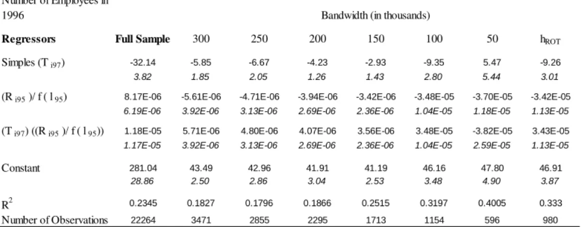
Tables A1 to A4 in the Appendix provide the estimated values for the coefficients considered as inputs for the parameters illustrated in Table 3. For the sake of comparability with the results derived from the second strategy we have restricted the sample to firms with gross revenues in the previous year close to the eligibility threshold (R$720,000 in 1996 and R$1,200,000 in 1998). To minimize the risk of having the results driven by an arbitrary definition of closeness, we have conducted all the estimations with several distinct bandwidths18.

Table 4 summarizes all the results from these tables by converting them to estimated values for all of the parameters (as opposed to coefficients) illustrated in table 3 for 1997 and 1999. We assume the following criterion to define the result to be reported among the various available alternatives (corresponding to different bandwidths): any component effect (total, composition or scale) for a given dimension (red tape cut or tax rate reduction) was considered statistically different from zero when that parameter was estimated as significantly different from zero in most of the bandwidths. In case of significance, Table 4 included the rule-of-thumb bandwidth result (h_ROT )19.

18

There is still no consensus in the RDD (our second strategy) literature about the definition of the optimum bandwidth size. In practical terms, Imbens and Lemieux (2008) suggest that the regression model should be estimated by varying the bandwidth size. In principle, the smaller the bandwidth, the better the estimation accuracy, provided that it has a sufficiently large number of observations. We considered bandwidth sizes of R$50,000 to R$300,000, in R$50,000 increments. In addition, we also estimated models using a rule-of-thumb (ROT) bandwidth as suggested by Lee and Lemieux (2009).

19

18

Table 4. Estimated Parameters of the SIMPLES Program Effect

Component\Dimension Red

tape Tax

rate Overall Red tape

Tax

rate Overall

1997 1999

Biased (total) effect _{null null null null null}

Bias (composition) _{-9.3 null -9.3 null null}

ATNT (scale effect) _{9.3 null 9.3 null null}

Note: Tables A1–A2 and A3–A4 in the Appendix refer to the biased and sample selection

effects, so that, the T_it and T_it

(

R_it−1/ f

( )

l_it−1

)

coefficients refer to red tape cut and tax

rate reduction effects, respectively.

We begin the results analysis with the first three columns of table 4, which report the results for 1997. From the first row, we can see that the overall effect of the scale and composition components is null in both mechanisms we consider (red tape cuts and tax rate reduction). The second and third rows report the results for the composition and scale effects, respectively.

We find evidence that the red tape simplification dimension of the program has a negative effect on firms' average employment level. This can be interpreted as suggested by our theoretical framework, which says that such simplification allows relatively inefficient and small firms to survive. This result is offset by a positive scale effect on firms' average employment level. That is, surviving firms convert the cost reduction allowed by red tape simplifications to an increase in their employment level, a tendency that is also suggested by the theoretical framework.

However, we get null results for the tax rate reduction dimension of the program, both in its scale and composition components. This result is predicted too by our theoretical framework. The firms do not change their employment level because of the tax rate, but they do decide not to survive based only on this benefit.

Our estimation for the overall effect of the program on average employment level in 1997 by each of the two components can be found in the third column. The results point to a negative composition and a positive scale effect, meaning that the red tape cut dimension of the program drives the overall effect in 1997. In terms of magnitude, these effects amount to 9.3 employees, meaning that simplifying the red tape procedures for tax payment would allow firms to employ 9.3 additional workers. Moreover the same simplification would allow smaller firms to survive, which in turn would lower the average employment level in the same sample size of workers20,21.

20

Concerning the magnitude of our estimated values, there are reasons to believe that both the scale and composition effects may be underestimated. Concerning the scale effect, it is possible that firms near the threshold may decide not to grow too much (in 1997/99) to avoid becoming ineligible for the program the next year (1998/2000). Concerning the composition effect, it is possible that the size composition of the treated group could also be modified by the entrance of new firms that would not have entered if SIMPLES had not been implemented.

21

19

The last three columns report the results for 1999, when the eligibility criteria were altered. The threshold value for gross revenue in the previous year was increased from R$720,000 to R$1,200,000. From this table we can see that the SIMPLES program had no effect on firms’ employment level22, irrespective of which dimension of the program (either red tape simplification or tax rate reduction) or which component of the effect (either scale or composition) is considered.

6.2. Second Estimation Procedure: FRD

In this section, we will discuss the results from the estimation procedure related to our second identification strategy. This estimation procedure relies on the FRD econometric framework, which in turn is implemented through an instrumental variable regression. As previously discussed, by using this method we are able to deal with the selection into the treatment group but not with the sample selection problem. Therefore, the estimand of this first step is the sum of the ATNT parameter and a sample selection term. In the previous section, we referred to this sum as the biased effect. Therefore, we can see this exercise as a robustness test for the first step of the previous estimation procedure, where the identification does not rely on a particular theoretical model.

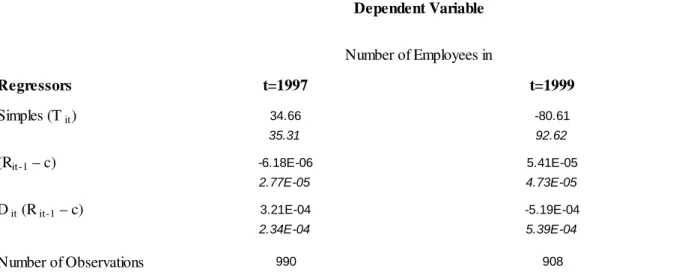
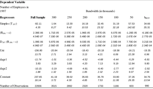
Table 5. Estimates for the FRD Model

Regressors t=1997 t=1999 Simples (T it) 34.66 -80.61

35.31 92.62

(Rit-1 – c) -6.18E-06 5.41E-05

2.77E-05 4.73E-05

D it (R it-1 – c) 3.21E-04 -5.19E-04

2.34E-04 5.39E-04

Number of Observations 990 908

Note: The estimates for all variables and bandwidths are in Table A5-A6.

We included as dummy regressors for subsectors of the industry, for states, for one establishment firms and for age groups. D i96 = 1, firm is eligible for SIMPLES in 1997 if 0<=(Gross Revenue in 1996)<=720000 e D i96 = 0 if (Gross Revenue in 1996)>720000.

Simples (T i97) = 1 if the firm opted for SIMPLES in 1997 and 0 if it did not;

(R i96 – c) = (Gross Revenue in 1996)-720000;

D i98 = 1, firm is eligible for SIMPLES in 1999 if 0<=(Gross Revenue in 1998)<=1200000 e D = 0 and (Gross Revenue in 1998)>1200000.

Simples (T i99) = 1 if the firm opted for SIMPLES in 1999 and 0 if it did not;

(R i98 – c) = (Gross Revenue in 1998)-1200000;

Standard Error in italics.

Number of Employees in Dependent Variable

Table 5 provides the estimated values for the parameters in equation FuzzyModel for both years considered in our sample. The estimated value of λ₂ corresponds to our estimation of the biased effect. From this table, such an effect is estimated to be null in both 1997 and 1999.

As the procedure here does not allow us to distinguish the red tape simplification dimension

the end of 1996 (1998). But we observed that only three (zero) firms demerged from 1996 (1998) to 1997 (1999).

22

20

of the program from the tax rate reduction dimension, we have to compare the estimated values of

2

λ with the overall biased effect estimated from the previous strategy. This value was also null for both years, providing further evidence that the scale and composition combined effect of the SIMPLES program on average employment level is null.

Thus, the evidence presented here suggests that, in 1997, firms with revenues close to the revenue threshold benefited from the SIMPLES program in two different ways. First, those that did not need the program to survive increased their employment level. Second, some of the less efficient firms that would have shut down had the program not been implemented remained active because of the benefits of the program. Both effects were due to red tape cuts, but not to the reduction in the tax rate. Therefore, in the first year after the law took effect, the firms took advantage of the higher efficiency level stemming from the bureaucracy simplification and hired more workers (scale effect), deciding to remain in the market one more period (composition effect). The tax cuts tended to not impact the average employment level either in the scale or composition dimensions. The FRD result showed that the total effect is really null and is the same as the first strategy, based on the theoretical model. The restrictions imposed by our theoretical framework seem not to distort the estimations.

7. Conclusions

In this paper, we have estimated the employment effect of a tax incentive program that targets small businesses in Brazil. Besides providing results for such unexplored questions, the main contribution in this paper was to combine a theoretical model of firm dynamics with longitudinal firm data to identify and estimate the carefully defined parameters that take into account two distinct dimensions of the program, red tape simplification and tax rate reduction, as well as two distinct transmission mechanisms that we named scale component and composition effects.

The results show that firms that chose to enroll in the SIMPLES program took advantage of the improved conditions under the program to employ more workers in 1997. That is the scale effect mentioned above. Contrarily, a firm’s average employment level tends to fall among treated firms in 1997 as the program managed to avoid the exit of small firms. This is the aforementioned composition effect. These two effects have a similar magnitude, providing a null aggregated effect on the average firm employment level. Both of these effects were driven exclusively by the red tape simplification dimension of the program.

The results for 1999 points to null effects, regardless of the mechanism and the program dimension considered. But, it is worth mentioning that our approaches provide local treatment effects. That is, this is a valid result for firms with revenue around the eligibility threshold value only. However, this evidence does not necessarily imply that smaller firms (in terms of revenue) do not take advantage of better conditions provided by the SIMPLES program by hiring more workers. Finally, a robustness exercise based on the FRD framework, and hence not depending on any structure imposed by our theoretical framework, confirms the null overall effect for both years.

References

Birch, D. L. (1987). Job Creation in America: How Our Smallest Companies Put the Most People to Work. New York: Free Press.

Brasil (2009). Indicadores de Equidade do Sistema Tributário Nacional. Brasília: Presidência da República, Observatório da Equidade.

Davis, S. J.; J. C. Haltiwanger and S. Schuh (1996). Job Creation and Destruction. Cambridge: The MIT Press.

21

of Empirical Research. International Tax and Public Finance, 10(6):673-93.

Fajnzylber, P.; Maloney, W. F. and Rojas, G. V. M (2011). Does formality improve micro-firm performance? Evidence from the Brazilian SIMPLES program. Journal of Development Economics, 94: 262-276.

Hasset, K. A. and R. G. Hubbard (2002). Tax Policy and Business Investment. In: Auerbach, A. and Feldstein, M. (Eds.), Handoobk of Public Economics, v.3. Amsterdam: Elsevier.

Imbens, G. and T. Lemieux (2008). Regression Discontinuity Designs: A Guide to Practice. Journal of Econometrics, 142(2): 615-635.

Klemm, A. and S. V. Parys (2009). Empirical Evidence on the Effects of Tax Incentives. IMF Working Paper.

Lee, D. and T. Lemieux (2009). Regression Discontinuity Designs in Economics. NBER Working Paper n.14723.

Lopez-Acevedo G. and M. Tinajero (2010). Impact Evaluation of SME Programs Using Panel Firm Data. Policy Research Working Paper, World Bank.

Monteiro, J. and J. Assunção (2009). Coming out of the shadows: estimating the impact of bureaucracy simplification and tax cut on formality and investment. Working Paper, Pontifícia Universidade Católica, Departament of Economics, Rio de Janeiro.

Moscarini, G. and F. Postel-Vinay (2009). The timing of labor market expansions: new facts and a new hypothesis. In: Acemoglu, D; Rogoff, K.and Woodford, M. (Eds.), NBER

Macroeconomics Annual.

Newmark, D.; B. Wall and J. Zhang (2011). Do Small Businesses Create More Jobs? New Evidence for the United States from the National Establishment Times Series, The Review of Economics and Statistics, 93(1): 16-29..

World Bank (2009). A Handbook for Tax Simplification World Bank Washington, D.C. World Bank (2010). Paying Taxes 2011: the Global Picture World Bank Washington, D.C.

8. Appendices

8.1. Proofs

8.1.1. Results on the survival decision in the theoretical model

A firm decides to continue whenever the present value of its expected profits is greater than any scrap value it gets when shutting down. That is, continuation requires:

. ] [

1 _>Ψ

−

∑

s

s

s

Eπ

ρ

The properties stated for E[u_t |u_t−1] and εt allow us to restate the condition above as:

(

1

)

. .ln( 1) . ] .

[ 1

1 ₋ ∗_{+ −} ∗ _>Ψ

− −

∑

s s t t s t

s

s

w u

p

τ ρ

(25)

It is easy to see that the left hand side increases monotonically with u_t−1; therefore, there

will be a unique value for this variable that will equate both sides of the equation above; this will be the first result to be proved here.