Aline Martines Piroutek
NOVOS MODELOS DE VIZINHANC
¸ A ESPACIAL E
Aline Martines Piroutek
NOVOS MODELOS DE VIZINHANC
¸ A ESPACIAL E
VIGIL ˆ
ANCIA PROSPECTIVA ESPAC
¸ O-TEMPO
Tese apresentada como requisito parcial para obten¸c˜ao de grau de Doutor em Estat´ıstica pela Universidade Federal de Minas Gerais.
Orientador: Prof. Dr. Renato Martins Assun¸c˜ao Co-Orientador:Profa. Dra. Denise Duarte
Programa de P´os-Graduac¸˜ao em Estat´ıstica Departamento de Estat´ıstica
...numa montanha vermelha vocˆe me resgatou. E, no cume de outra, sonho em te reencontrar...
PARA MINHA M ˜AE, OLGA,
Agradecimentos
A trajet´oria de um aluno de doutorado ´e bastante longa e ´ardua. Sozinhos, n´os n˜ao seriamos capazes de alcan¸car essa vit´oria. Sim, digo vit´oria. Vit´oria, primeiro pela ansiedade para ingres-sar no programa. Vit´oria, por conseguir estudar de madrugada disciplinas antes assumidas por outros n˜ao ”condizentes”com nossas capacidades. Vit´oria, pelo esfor¸co em aprender e a tornarmos profissionais em busca de nossas ”curiosidades cient´ıfica”. Agrade¸co a Deus que, atrav´es de v´arias pessoas em nossa volta, nos mostra o caminho e nos fortalece com sua bondade. Devo agradecer ao meu pai Mirko, pela apoio incondicional. N˜ao sei como poderia ir em frente sem esse exemplo de vida. Pessoa dedicada a fam´ılia e que se esfor¸ca integralmente para nosso sucesso. Fique tranquilo, pois vocˆe fez e faz muito mais do que o suficiente. `As minhas irm˜as, eu tamb´em agrade¸co... `A T´alita e seu ”sub-bloco”(Andr´e, Carol e Daniel) por serem minha segunda casa. Obrigada pelo momentos bons e por me acolher nesse novo lar. Sempre poderei aprender com os mais experientes e desfrutar da alegria das crian¸cas. `A J´essica, minha irm˜a mais nova, agrade¸co pela alegria e pelo carinho. Obrigada por me esperar voltar para casa e querer passar um tempo comigo. Obrigada por me escutar falar de mim mesmo quando eu n˜ao te deixava falar de vocˆe. Sei que as vezes vocˆe sofre e acha que n˜ao ´e valorizada, mas saiba que sinto muito orgulho de todo seu talento e de suas conquistas.
Resumo
Abstract
vi to practical use by public health official agencies. Our method is a modification from a previous proposal made by Rogerson, who examined a retrospective surveillance scenario, looking for the earliest time in the past that change could have been deemed to occur. We modify his method to take into account the prospective case. We evaluated our surveillance system in several scenarios, including without and with emerging clusters, checking distributional assumptions and assessing performance impacts of different emergence times, shapes, extent and intensity of the emerging clusters.
Palavras-chaves: Estat´ıstica espacial, mapeamento de doen¸ca, campos de Markov, modelos
espa-ciais hier´arquicos, vigilˆancia prospectiva espa¸co-tempo, cluster espa¸co-tempo, ´arvores de contexto,
Introdu¸
c˜
ao
A presente tese de doutorado apresenta resultados de investiga¸c˜oes complexas e aprofundadas na ´area de Estat´ıstica Espacial.
Trata-se, em verdade, de trˆes trabalhos independentes e autˆonomos, e em raz˜ao de terem sido submetidos `a publica¸c˜ao no exterior, encontram-se em formato de artigos - raz˜ao pela qual dois deles foram redigidos em inglˆes.
A primeira parte ´e intitulada ”Non-Homogeneos Probabilistic Context Neighborhood estimation on two dimensional lattice by pruning spanning trees”, no qual exploramos m´etodos de estima¸c˜ao de probabilidades de transi¸c˜ao em Campos de Markov (Markov Random Field - MRF).
Assim como ocorre com as cadeias de Markov, a modelagem dos MRFs torna-se um problema quando o n´umero de sites vizinhos ´e elevado.
Rissanen (1983) introduziu, para casos unidimensionais, a ideia de mem´oria vari´avel em modelos PCT, na qual a predi¸c˜ao do pr´oximo s´ımbolo depende t˜ao-somente da parte relevante de seu passado (contexto). Assim, o contexto de cada site varia segundo os valores de seus s´ımbolos antecessores. O m´etodo permite, ainda, a representa¸c˜ao do conjunto de contextos a partir de uma ´arvore, que sumariza toda a estrutura de dependˆencia do passado de uma cadeia de Markov.
Existem outros estudos focados nos processos MRFs. Ao utilizarem o Pseudo-Bayesian Infor-mation Criterion (PIC), Csiszar and Talata (2006) prop˜oem um estimador fortemente consistente nas realiza¸c˜oes de uma crescente regi˜ao finita. Locherbach, por sua vez, denomina esse processo de Variable Neighborhood Random Field (VNRF), estendendo o conceito de contexto (ou vizin-han¸ca de contexto) para um lattice com r-dimens˜oes propondo um estimador para o raio de uma vizinhan¸ca b´asica (o menor c´ırculo que cont´em o contexto do site).
viii ideias de vizinhan¸ca vari´avel em um lattice, estima¸c˜ao do PCT para casos unidimensionais e uso do PIC como crit´erio de sele¸c˜ao. Al´em disso, propusemos uma nova geometria para as vizinhan¸cas de contexto, variando o raio da estrutura (segundo os valores que apresenta). Esse nova geometria permite uma dr´astica redu¸c˜ao de parˆametros livres e torna poss´ıvel o c´alculo da cardinalidade do conjunto de vizinhan¸cas de contexto.
Nosso modelo, chamado de Probabilistic Context Neighborhood (PCN), possibilita representar graficamente a estrutura de dependˆencia das vizinhan¸cas atrav´es de uma ´arvore - aspecto funda-mental para o entendimento do comportamento de intera¸c˜oes. Prop˜oe, ainda, um algoritmo de estima¸c˜ao das vizinhan¸cas de contexto gerado por um PCN. Apresenta, por fim, um m´etodo de regionaliza¸c˜ao para os cen´arios em que as PCN n˜ao s˜ao homogˆeneas ao longo do lattice (Non-Homogeneous Probabilistic Context Neighborhood - NHPCN), decorrente de uma adapta¸c˜ao do Spatial ’K’luster Analysis by Tree Edge Removal (Skater). Para possibilitar o m´etodo de regional-iza¸c˜ao, propusemos trˆes medidas de dissimilaridades entre ´arvores (probabilidade, complexidade e estrutura).
Ressalte-se que toda a metodologia desenvolvida no trabalho apresentou resultados satisfat´orios nas simula¸c˜oes.
ix adas piroris, na qual ser´a poss´ıvel fazer inferˆencias atrav´es de m´etodos computacionais (MCMC). Al´em disso, propusemos dois estimadores a posteriori, para a estrutura de vizinhan¸ca. Foram ap-resentados v´arios exemplos, simula¸c˜oes e aplica¸c˜oes do nosso m´etodo, cujos resultados foram mais satisfat´orios quando comparados ao modeloCAR.
Por ´ultimo, apresentamos o trabalho intitulado ”Space-time prospective surveillance based on Knox local statistics”, o qual aborda m´etodos prospectivos na detec¸c˜ao de clusters espa¸co-tempo.
Os m´etodos de vigilˆancia espa¸co-tempo podem ser divididos em duas categorias: aqueles que usam dados de ´areas e os que usam dados pontuais. Dentre os primeiros, vale ressaltar o estudo desenvolvido por Raubertas (1989) - o qual descreve procedimentos anal´ıticos e a sua implementa¸c˜ao na epidemiologia e na sa´ude p´ublica. Kulldorff (2001), por sua vez, prop˜oe a estat´ıstica scan para o monitoramento cont´ınuo de doen¸cas em dados de ´areas, a qual foi adaptada pelos Neill et al.(2005), Kulldorff et al. (2005) e Assun¸c˜ao et al. (2007) e criticada por Woodall et al. (2008).
Para a categoria de dados pontuais, podemos mencionar o trabalho de Assun¸c˜ao and Correa (2009) , o qual n˜ao exige a especifica¸c˜ao das fun¸c˜oes puramente espacial e temporal. A proposta dos autores consiste em adaptar o m´etodo gr´afico de controle introduzido por Shiryayev-Roberts para a situa¸c˜ao espa¸co-tempo e utilizar o Optional Stopping Theorem para obter os valores dos parˆametros de ajuste do m´etodo.
Rogerson (2001), por sua vez, prop˜oe a utiliza¸c˜ao individual dos pontos geo-referenciados dos eventos nos c´alculos da estat´ıstica de Knox local. Trata-se de m´etodo retrospectivo apresentando significativas vantagens em rela¸c˜ao a seus antecessores: baseia-se em uma estat´ıstica intuitiva (Knox local); n˜ao necessita de conhecimento pr´evio na sua aplica¸c˜ao; desnecessidade de modelar as fun¸c˜oes marginais de padr˜ao espacial e temporal; e seus parˆametros s˜ao interpret´aveis e facilmente fixados. Marshall (2007) estuda o m´etodo de Rogerson atrav´es de simula¸c˜oes, sob a hip´otese de ausˆencia de clusters. Ao avaliar o efeito do average run length (ARL) em cen´arios diversos, o autor encontra diversos problemas na estat´ıstica de knox local, raz˜ao pela qual n˜ao recomenda a utiliza¸c˜ao do m´etodo para aplica¸c˜ao em casos reais.
x um dado aspecto da doen¸ca em an´alise. Tamb´em checamos a distribui¸c˜ao exponencial dos ARL0 assumida por Rogerson. Observamos, ainda, que a aproxima¸c˜ao para o c´alculo do limiarhfunciona bem quando existem pelo menos seis eventos dentro da ´area de busca. Al´em disso, as conclus˜oes obtidas a partir das simula¸c˜oes s˜ao v´alidas tanto para cen´arios com densidade populacional ho-mogˆenea e como para cen´arios com densidade n˜ao hoho-mogˆenea. Da mesma forma, as simula¸c˜oes em cen´arios sob a hip´otese de cluster apresentaram os resultados esperados.
Non-Homogeneous Probabilistic Context Neighborhood
estimation on two dimensional lattice by pruning
spanning trees
A. Pirouteka, D. Duartea,∗, R. Assun¸c˜aob,
a
Departamento de Estat´ıstica, Universidade Federal de Minas Gerais, 31270-901. Belo Horizonte, MG, Brazil
b
Departamento de Ciˆencia da Computa¸c˜ao, Universidade Federal de Minas Gerais, 31270-010. Belo Horizonte, MG, Brazil.
Abstract
We introduce the Probabilistic Context Neighborhood model for two
dimen-sional lattices as an extension of the Probabilistic Context Tree model in one
dimensional space preserving some of its interesting properties. This model
has a variable neighborhood structure with a fixed geometry but varying
radius. In this way we are able to compute the cardinality of the set of
neighborhoods and use the Pseudo-Likelihood Bayesian Criterion to select
an appropriate model given the data. We represent the dependence
neigh-borhood structure as a tree making easier to understand the model
com-plexity. We provide an algorithm to estimate the model that explores the
sparse tree structure to improve computational efficiency. We also present an
extension of the previous model, the Non-Homogeneous Probabilistic
Con-text Neighborhood model, which allows a spatially changing Probabilistic
∗
Corresponding author
Context Neighborhood as we move on the lattice.
Keywords: Context tree, Markov random fields, Variable-neighborhood
random fields, Context algorithm, Probabilistic context trees, Model
selection.
1. Introduction
In this paper we are concerned with the task of providing transition
prob-ability estimators for Markov random fields (MRF) on a two dimensional
lattice by using a specific kind of neighborhood geometry with variable size.
We mean by neighborhood the minimal region that determines the
condi-tional distribution of a site subject to the values of all other sites. We also
address the problem of model selection inside a class of MRF with variable
neighborhood structure.
The Markov random field (MRF) on lattices is a model that has been
increasingly exploited nowadays. It has for example several applications in
computing. We can mention the image processing, which includes
recogni-tion, segmentarecogni-tion, image compression and restoration ([1], [2], [3], [4] and
[5]). In statistical physics, the MRF is essential for modeling interactive
par-ticle systems [6]. In sociology, we can see several applications in polarization
phenomena in society and in social networks [7]. In the area of machine
learning the MRF are used in the search for hidden patterns, called learning
structure [8].
Markov chain modeling could become a problem when the order
depen-dency is not small because, in this case, the number of parameters to estimate
in the neighborhood to be very large, since for each site in the lattice is
as-sociated a conditional probability that this site assumes a value according
to the values showed in its neighborhood. Besides that if the neighborhood
structure is fixed all over the lattice it is not possible to allow bigger
depen-dency for sites in one region than in another. This can be a serious restriction
for modeling some spatial phenomena for example.
One possible solution to this problem is to consider a variation of the MRF
model analogous to Variable Length Markov Chain (VLMC) or Probabilistic
Context Tree (PCT) initially proposed for Markov chains.
The PCT model for one-dimensional data was introduced by [9] in
in-formation theory for binary codes. He introduced the notion of variable
memory which means that in order to predict the next symbol is not
nec-essary to keep in memory all the past. The relevant part of the past called
”context” can vary from one sequence to another. In this way the set of
contexts can have substrings of different sizes and can be represented as a
tree. This tree representation is very useful to understand the dependency
structure of the source on the past. Processes of this class are still Markovian,
but with variable memory length, producing a class of models structurally
larger and richer than Markov chains of fixed order. He also introduced the
context algorithm to estimate PCT which is able to compress long strings
generated by a source.
In theoretical studies, we mention the work of [10], which established
new results in processes of infinite dependence trough an adaptation of the
Context algorithm. The consistency and some properties of BIC context tree
digital contours is considered in [15]. They studied the problem of the chain
codes of digital contours in map images. They applied the context tree based
approach and provided an optimal algorithm for n-ary incomplete context
tree construction. Several studies contributed to this literature in various
directions [16], [17] and [18]. In a practical level, we could mention its usages
in information theory, focusing on bioinformatics [19], [20], linguistics [21]
and universal coding [22].
For MRF processes [23] propose an estimator for a basic neighborhood,
based on a modification of the Bayesian Information Criterion (BIC)
replac-ing likelihood by pseudo-likelihood. They also prove that this estimator,
called Pseudo-Bayesian Information Criterion (PIC), under certain
condi-tions is strongly consistent for a realization of a field in a growing finite
region.
This kind of processes is called Variable Neighborhood Random Field
(VNRF) model in [24] where the concept of ”context” is extended to a
r-dimensional lattice. They propose an estimator for the radius of the basic
neighborhood (context) of a site, i.e., the smallest circle containing the
con-text of the site. They still define an algorithm to estimate this radius, and
prove the consistency of the estimator.
In this work we propose a different kind of context neighborhood geometry
for the MRF. We fix a frame structure for neighborhoods of a site and allow
the radius of theses frames to vary according to the values presented in
the frame. The advantage is that with this geometry the number of free
parameters is reduced and we are able to compute the cardinality of the set
to obtain an optimal model given the sample and we also present a graph
representing the variable neighborhood structure in a tree format analogous
to the one dimensional PCT. We call this model as Probabilistic Context
Neighborhood (PCN). Based on this approach we propose an algorithm for
estimating the context neighborhoods of a two-dimensional lattice generated
by a PCN source. We apply our methodology to simulated data in order to
show how well it recovers the parameters of the model.
Besides the estimators for the PCN model and the PCN model
selec-tion procedure we also propose a regionalizaselec-tion method when the PCN is
not homogeneous on the entire lattice. We allow the PCN source
gener-ating the data to vary from one region to another. We call this model as
Non-Homogeneous Probabilistic Context Neighborhood (NHPCN). This is
done from an adaptation of the Skater method, standing for Spatial ’K’luster
Analysis by Tree Edge Removal ([25], [26]), through measures of dissimilarity
between trees estimated in different regions of the lattice. [27] proposed an
automatic learning of a non-parametric stochastic tree edit distance (ED) to
learn the optimal edit costs. They proposed two probabilistic approaches.
The first one uses the joint distribution over the edit operations and builds a
generative model of the tree ED. The second gives a discriminative model by
using a conditional distribution. Unlike dissimilarities commonly used [28],
in our work we propose dissimilarity between PCN based on the complexity,
structure and conditional probabilities of the PCN from each region.
Finally, we make a simulation study to analyze the adequacy of our work
in practice to black and white images. First, we present an example
the probabilities of a two-dimensional Ising model [29]. In a second step, we
focus our simulations on the recovery of the NHPCN from a sample generated
by two different PCN’s in distinct regions of the lattice. The first PCN has
only one generation, i.e., the value of the site depends only on the first order
neighborhood. The second tree has variable neighborhood degrees (first and
second order). In our results, we found that our model was able to recover
the real tree. This allows us to believe that our method is feasible and useful
in practice.
2. Definitions
Let us consider a two dimensional latticeZ2. The pointsi∈Z2 are called
sites or areas, where||i||denotes the maximum norm ofi, i.e. for i= (i1, i2),
||i||= max(|i1|,|i2|) is the maximum of the absolute values of the coordinates
of i. The cardinality of a set ∆ is denoted as |∆|. We denote by ⊂ and ⋐
the inclusion and strict inclusion, respectively. Subsets ofZ2 will be denoted
by uppercase Greek letters. Thus, if Λ is a finite set of sites, then Λ⋐Z2.
A random field is a family of random variables indexed by the site i of
a lattice, {X(i) : i ∈ Z2}, where each X(i) is a random variable that takes
values in a finite discrete alphabetA. We denote the set of all configurations
of the random field as Ω =AZ2
. For realizations ofX(∆), we use the notation
a(∆) ={a(i)∈A:i∈∆}.
The joint distribution of the variablesX(i) is denoted as Q:
Q(a(∆)) =P(X(∆) =a(∆))
for ∆⊂R2 and a(∆) ∈A∆.
In turn, the definition of conditional probability is given by:
Q(a(∆)|a(Φ)) =P(X(∆) =a(∆)|X(Φ) =a(Φ))
,
for all disjoint regions ∆ and Φ where Q(a(Φ))>0 .
We say that the process is a Markov random field if there exists a
neigh-borhood Γi, satisfying for every i∈R2
P(X(i) = a(i)|X(Z2\i) =a(Z2\i)) =P(X(i) =a(i)|X(Γi)) =a(Γi)). (1)
Where by a neighborhood Γi (of the site i) we mean a finite,
central-symmetric set of sites with i /∈Γi.
We consider a particular type of neighborhood which we call a frame
∂ij defined as a square of side 2j + 1 less a square of side 2j −1 with the same center i, for j ∈ N. We observe that for j = 1,2, ..m the frames ∂j
i
are nested sets in the sense that ∩m
1 ∂
j
i = ∅ and
∪m
1 ∂
j
i is a square region
of the lattice with center in the site i and side 2m + 1. In this work we
consider Γ(i) = ∂ij. Since the geometry of the neighborhood is fixed we only need to know j, the order of the neighborhood, to get the conditional
probabilities for a given sitei. To simplify notation sometimes we write only
∂j omitting the siteiwhenever it is clear. We say that a configurationa(∂j i)
is a realization of the process on the subset ∂ij. We also denote the union of frames ∪n
s=m∂s = (∂m∂m+1. . . ∂n) as ∂m,...,n. The concatenation of the
two configurations a(∂1,...,k) and a(∂m,...,n) is denoted by a(∂1,...,n), which is
Then we say thata(∂1,...,k) is a suffix of a(∂1,...,n) if a(∂1,...,n) is a
concate-nation ofa(∂1,...,k) anda(∂k+1,...,n). This defines a order in the space of
config-urations denoted by a(∂1,...,n)≽a(∂1,...,k). If the cardinality |a(∂n,...,m)| ≥0,
then the a(∂1,...,k) is a proper suffix.
Definition 1. The subset T ⊂ ∪∞
j=1A∂
1,...,j
is a neighborhood tree if no
a(∂1,...,j)∈ T is a suffix of any other a(∂1,...,k)∈ T for j < k∈N.
When a neighborhood tree does not contain proper suffixes it is called
irreducible and denoted by T ∈ I. The depth of a neighborhood tree is
defined as d(T) =maxj{∂j ∈ T }.
Definition 2. A finite configurationa(∂j)∈A|∂j|
is a context neighborhood
of a Markov random field if Q(a(∂j)>0 and
P(X(i) =a(i)|X(Z2\i) =a(Z2\i)) = P(X(i) =a(i)|X(∂j) =a(∂j))
= Q(a(i)|a(∂j))
(2)
for every i ∈ R2 and j ∈ N. We say that j is the order of the context
neighborhood a(∂j).
This means that the site i depends only on ∂j and there is no need to
inspect the entire lattice to decide the value assumed by X(i). If P satisfy
2, we call this process as Probabilistic Context Neighborhood (PCN).
A set of all context neighborhoods is a neighborhood tree and we denote
context neighborhood is fixed, the only variation is in j unlike [23] and this
implies that we have much less parameters in the model.
Our goal is to estimate the orderj of the context neighborhood of a site
i, considering that it may change from one site to another according to the
change in configurations.
In Figure 1 we can see the structures of neighborhoods of first to third
order. Bigger orders may be understood analogously.
From now on we focus on the space of binary states due to its simplicity
and because it allows the study of the interesting case of black and white
images. An extension to larger state spaces is straightforward. Besides that
we consider that only the number of black (or white) sites in the frame is
sufficient to provide the conditional probability given the configuration. This
is not a restriction in the model and could be easily changed. It is instead an
illustration of the model to more realistic situations such as in Ising Model.
Figures 2 and 3 are examples for a lattice withA={−1,1}, whereX(i) =
-1, if the observed value of sitei is white, and X(i) = 1 if it is black.
By using this type of neighborhood it is possible to draw a PCN analogous
to a PCT in one dimensional case as can be seen in the example of Figure 4.
We observe that the PCN preserves several of the characteristics of the PCT.
We list some of them in the following. Its root is drawn on top of the tree
and represents the value of the site i. The first generation node are drawn
from the root down and represents the first order neighborhoods. If the first
order information is not sufficient to provide a conditional probability for a
site then the second order neighborhood is drawn adding a frame to this first
Figure 1: Structure neighborhood for j = 1,2 and 3 respectively.
an added frame.
In the example showed in Figure 4 we can see that the PCN has context
neighborhoods of order 1, 2 and 3. There are seven context neighborhood of
the first order with 0, 1,2,4,5,7 and 8 black sites respectively (neighborhoods
with 3 and 6 black sites are not contexts). Therefore, if we observe only
one black site in the neighborhood, the probability of the site being black
is known. The same is true for 0, 2, 4, 5 and 8 black sites. If in the first
order neighborhood there are 3 or 6 black sites we must continue ”down” in
the PCN and look at the configurations of the second order. Once we did
that, we noticed that the configurations of the first order with 3 and 6 black
sites have 3 and 5 children respectively. The children of the configuration
Figure 2: Possible realizations for a first order structure
Figure 3: Possible realizations for a second order structure
not all children of the configuration with 6 black sites are considered context
neighborhood. There is a child (with 8 black sites) which also has children.
In Figure 4 we note that their children have 0 and 4 black sites in the third
order and are context neighborhoods. In summary, this PCN has a total of
16 context neighborhoods where 7 of which have first order, 7 have second
order and 2 have third order. For each context neighborhood a conditional
probability of the central site being black (or white) is assigned.
Figure 4: Example of a Probabilistic Context Neighborhood of order 3.
the frame (∂1) ⊂ (∂1,2). This pattern is repeated for all the orders of the
PCN, see Figure 4.
In this work, we focus on the estimation of the context neighborhood of
the true T0, from observations of a realization of a Markov field in a finite
region. This sample will be denoted as the a(Λn) and represents the set of n
sites under study.
Definition 3. Given a sample a(Λn), the pseudo-likelihood function
asso-ciated with the PCN T and the probability transition function Q is given
by:
P LT(a(Λn)) =
∏
a(∂1,...,j)∈T,N
n(a(∂1,...,j))>1
∏
a(i)∈A
Q(a(i)|a(∂1,...,j))Nn(a(∂1,...,j,i))
,
(3)
where
represents the number of times that the configuration a(∂1,...,j), is
ob-served in the sample when the siteiassumes the valuea(i) andNn(a(∂1,...,j))
is the number of occurrences of the configuration a(∂1,...,j) in the sample
a(Λn),
Nn(a(∂1,...,j)) =|{i∈a(Λn) :a(∂1,...,j)⊂a(Λn)}|.
The estimator that maximizes the pseudo-likelihood is given by:
ˆ
Q(a(i)|a(∂1,...,j)) = Nn(a(∂
1,...,j, i))
Nn(a(∂1,...,j))
.
Thus, given a samplea(Λn), the maximum pseudo-likelihoodM P LT(a(Λn))
is the pseudo-likelihood function evaluated at its maximum:
M P LT(a(Λn)) =
∏
Nn(a(∂1,...,j))>1
∏
a(i)∈A
Nn(a(∂1,...,j, i))
Nn(a(∂1,...,j))
Nn(a(∂1,...,j,i))
, (4)
Definition 4. Given a samplea(Λn), the PIC (Pseudo-Bayesian Information
Criterion) for a PCN T is:
P ICT(a(Λn)) =−logM P LT(a(Λn) +
(|A| −1)|T |
2 log|Λn|,
we stress that, unlike [23], here it is possible to obtain a simple, closed
formula for the penalty term since.
|T |=
maxja(∂1,...,j)∈T
∑
k=1
|A||a(∂k)|=
maxja(∂1,...,j)∈T
∑
k=1
|A|8k (5)
Given a samplea(Λn), a feasible PCNT is such that the order j ≤D(n),
a(∂j)∈ T. Besides that each configuration a(∂k) withN
n(a(∂k))≥1 ,k < j
is a suffix of some a(∂j) ∈ T . A family of feasible PCN is denoted by
F1(a(Λn), D(n)).
Definition 5. We define the PIC estimator of a PCN by
ˆ
TP IC(a(Λn)) = argminT ∈F1(a(Λn),D(n))∩IP ICT(a(Λn)),
The consistency of the estimator ˆQ(a(i)|a(∂1,...,j)) is a consequence of the corollary 2.1 in [23] in which they state the consistency of this kind of
estimator for a bigger class of possible neighborhoods provided that D(n) =
(log(Λn))1/4. Under this assumption they also prove the consistency of the
PIC estimator for each neighborhood Γ.
Simulation results presented in section 3 leads us to believe that due to
simplicity of the frame geometry structure ifD(n) =O(log|Λn|) the estimator
ˆ
TP IC is consistent because we are able to recover the real neighborhood tree
using this value.
2.1. Estimation Procedure
According to equation 4, the pseudo maximum likelihood function could
be factored as
M P LT(a(Λn)) =
∏
a(∂1,...,j i )∈T
˜
PM P L,∂1,...,j
i (a(Λn)), where
˜
PM P L,∂1,...,j
i (a(Λn)) =
∏
a(i)∈A
Nn(a(∂i1,...,j,i))
Nn(a(∂i1,...,j))
Nn(a(∂1i,...,j,i))
if Nn(a(∂i1,...,j))≥1
Using this factorization, we can rewrite the estimator ˆTP IC(a(Λn)) as
ˆ
T(a(Λn)) =argmaxT
∏
∂i1,...,j∈T
˜
P∂1,...,j
i (a(Λn)),
where ˜P∂1,...,j
i (a(Λn)) =n |A−1|
2 P˜
M P L,∂i1,...,j(a(Λn)).
This fact allows the computational treatment for the PIC estimator from
an extension of the CTM algorithm [22], [30]. The CTM algorithm is
de-scribed as follows:
Given a samplea(Λn), we assign to each node a value and a binary
indi-cator. This assignment is recursive, i.e., the value and the indicator assigned
are calculated from the values assigned to the children of this node. The
in-dicator determines the estimator, which assumes a sub-tree form, as follows:
Definition 6. Given a sample a(Λn), each node (neighborhood) received
recursively, from complete tree leaves , the value
V∂D1,...,j(a(Λn)) =
max{P˜∂1,...,j(a(Λn)) , ∏
a(i)∈A,Nn(a(∂1,...,j,i))≥1V
D
∂1,...,j,i(a(Λn))},
if 0≤j < D
˜
P∂1,...,j(a(Λn)), if j =D
(6)
and the indicator
χD∂1,...,j(a(Λn)) =
1 if P˜∂1,...,j(a(Λn))<∏
a(i)∈A,Nn(a(∂1,...,j,i)≥1V
D
∂1,...,j,i(a(Λn))
and 0≤j < D
0 if P˜∂1,...,j(a(Λn))≥∏
a(i)∈A,Nn(a(∂1,...,j,i)≥1V
D
∂1,...,j,i(a(Λn))
and 0≤j < D
0 if j =D
where D=D(n).
The pruning procedure is done starting from the root. If any of the first
order neighborhood result in an indicator equal to zero, we keep these nodes
and cut the entire second order configuration, which are connected to it. In
other words, we exclude children that have parents with indicator equal to
zero. We adopt the same procedure to the second order generation nodes that
were not pruned: by cutting the third order configuration that has parents
with indicator equal to zero. After the pruning procedure, all the nodes of
the resulting tree have indicator equal to one and all leaves have indicator
equal to zero [12].
2.2. Non Homogeneous Probabilistic Context Neighborhood- NHPCN
In section 2 we propose the PCN model for the two-dimensional lattice,
and described a computational method to estimate the PCN from a sample
a(Λn). By applying this methodology, we are able to estimate a single PCN
that represents the generating source for all sites in the sample. We now
present a model that allows us to have different PCN’s according to the sub
region of the lattice. We let the conditional probabilities of a site depend not
only on the neighborhood but also on the sub region of the lattice in which
the site is located.
Definition 7. Consider a partition of the lattice such that Λn = ∪mk=1∆k,
m ≤n, ∆k∩∆l=∅ for all k and l. For each subregion ∆k and i∈∆k
P∆k(X(i) =a(i)|X(Z
2\i) = a(Z2\i)) = P
∆K(X(i) =a(i)|X(∂
= Q∆k(a(i)|a(∂
j)),
(8)
where a(∂j) is a context neighborhood. We call this process as
Non-homogeneous Probabilistic Context Neighborhood (NHPCN).
Then in this model we have that
• Sites of the same sub-region should become from the same PCN.
• Sites of different sub-regions should become from dissimilar PCN.
Thus using a NHPCN one might ask if the PCN representing the north
of a region is not equal to the PCN representing the south. The same for
east and west. But two adjacent sites could have been generated from the
same PCN or from a similar PCN.
Our goal now is to propose a procedure for grouping sites into
homoge-neous and contiguous regions. Thus each region would contain a set of sites
governed by the same PCN, and different regions will have different PCN.
The problem is to find the appropriate partition of the sample. To solve
this problem, we use the SKATER (Spatial K’luster Analysis by Tree Edge
Removal) method, suggested by [26], that transforms a region (or lattice)
into a graph and splits this graph according to the cost of keeping its edges
together [31]. We propose to use a cost based on PCN dissimilarities.
2.3. NHPCN Estimation
In this section we describe the strategy to transform the regionalization of
a lattice in a problem of graph partitioning, through the SKATER algorithm
We represent the region of interest through a graph G = (V, E) where
each sitei is represented by a node (or vertice)vi and two neighboring sites,
i and j, are connected by an edge (or line) (vi, vj). We denote V as a set of
vertices and E as a set of edges of the graph G. In the present work, two
areas are considered neighbors if they have a common border. Apath ofvito
vk is a sequence of distinct nodes vi, vj, . . . , vk which are connected by edges
(vi, vj),(vj, vl), . . . ,(vm, vk). A graph is connected if, going from a nodevi to
any other node vj, there is at least one path fromvi tovj.Acycle in a graph
is a path where the start node and the end node are the same. A tree is a
graph that does not have cycles.
A spatial cluster is a subset of connected sites. A region is partitioned
into spatial clusters when they are disjoint. Our goal is to partition the graph
G into cspatial clusters G1, G2, ..., Gc, where ∪c
kGk =G.
A spanning tree (ST) of a graph G is a tree connecting all the n sites of
G, whereas two sites are connected by one single path and the number of
edges is n−1. Removing an edge from the tree, we have two sub-graphs
connected which are candidates to become spatial clusters.
Each sitei, i= 1, . . . , n, has a vector of attributes (characteristics) given
by bi = {b1i, . . . , bmi}. We associate a cost d(i, j) between the sites (i, j)
as the measure of the dissimilarity among these sites through bi and bj.
The measure of dissimilarity depends on the situation. When the attributes
have comparable scales, a usual choice is the Euclidian distance between
the vectors of attributes bi and bj. A minimum spanning tree (MST) is
a spanning tree with minimal cost, where cost is measured as the sum of
its neighbors are distinct, the MST is unique [32].
The MST is obtained from the graph by the Prim algorithm [33].
In our problem, the attribute of each site is a PCN, as we proposed in
section 2. Considering all these concepts, the SKATER procedure can be
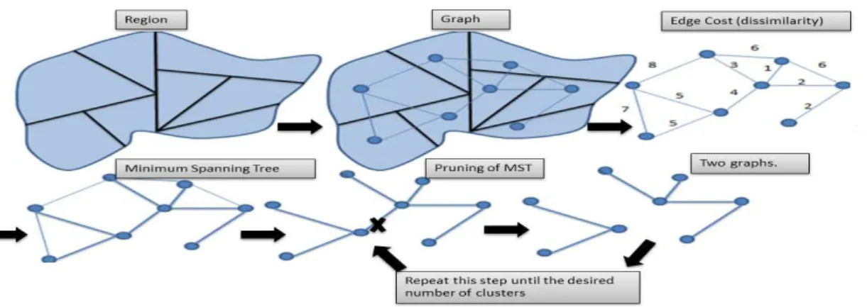
described in 5 steps:
1. Turn the lattice into a graph;
2. Calculate the cost of the edges (dissimilarity);
3. Reduce the graph to a minimum spanning tree [31] ;
4. Prune the MST and
5. Repeat the previous item until the desired number of clusters is reached.
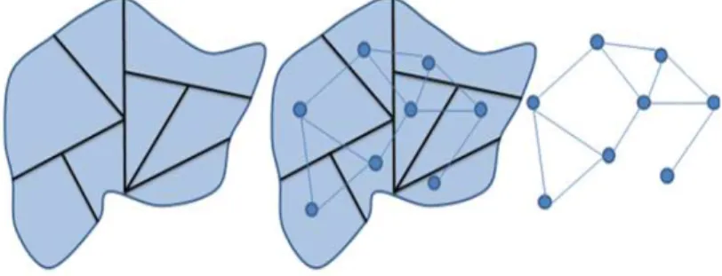
Figure 5 shows a scheme of the procedure.
Figure 5: Procedure Skater
We are going to explain the procedure in more details in the following
section.
2.3.1. Pruning the MST
After construction of the MST, we move to a step in which we are going
necessary to remove c−1 edges of the tree. Each cluster will be a resulting
tree connected to all sites, without cycles.
To create a partition ofnsites inctrees, we use a strategy of hierarchical
division. Initially, all sites belong to a single tree. As the edges of the MST
are removed, a set of trees appears disconnected. At each iteration, a tree
is divided into two trees by cutting an edge, until we reach the number of
clusters previously stipulated.
In this step, to allow more homogeneous and balanced regions in terms
of number of sites, the cost is given by:
Edge cost l=SSDTM ST −SSDl,
where
SSDM ST is the sum of squares of deviations associated with the MST,
given by:
SSDM ST = m
∑
j=1
nM ST
∑
i=1
d(bij −¯bj),
where nM ST is the number of sites the MST, bji is the value of the j
-th attribute of -the site i; m is the number of attributes considered in the
analysis and ¯bj is the average value of j -th attribute in all sites of MST.
SSDl is the sum of two parts, M ST1 and M ST2, of the two sub-trees
generated by the removal of the edge l oh the MST:
SSDl=SSDM ST1 +SSDM ST2
calcu-lated the average values of mattributes in the same way as in the calculation
of SSDM ST but considering only attributes related to objects belonging to
each sub-tree of M ST,M ST1 and M ST2.
After finding each edge cost we remove the one that has minimum cost.
Then we repeat the process on each of the sub-tree until a stopping criterion
is reached (for example, the desired number of classes).
2.3.2. Dissimilarity between PCN’s
The SKATER method is used to make a regionalization of the sample into
sub regions. We note that it is possible to work with a vectorb={b1, . . . , bm}
for each site. In our work, we will consider as an attribute a sub-PCN as
defined in section 2. Thus for each sitei,i= 1, ..., nwe define a PCN Ti such
that
• Ti represents a PCN for a sub-lattice centered in the siteiwith a square
geometric shape and base equal to m.
• Ti has the same properties of the PCN previously defined.
After setting the attribute of each site we define a dissimilarity measure
between them given by.
d(Ti,Tj) = w1ds(Ti,Tj) +w2dp(Ti,Tj) +w3dc(Ti,Tj) (9)
where 0≤ wk ≤1 , ∑3k=1wk = 1 , ds(Ti,Tj) represents the difference in
structure,dp(Ti,Tj) the difference in probability, anddc(Ti,Tj), the difference
ds(Ti,Tj) =
{a(∂
1,...,k)∈ T
i}∆{a(∂1,...,l)∈ Tj}
|{a(∂1,...,k)∈ T
i}|+|{a(∂1,...,l)∈ Tj}|
, (10)
dp(Ti,Tj) =
1 2|A||{a(∂1,...,l)∈(T
i∪ Tj)}|
×
∑
a(k)∈A,a(∂1,...,l)∈(Ti∪Tj) (
Nni(a(∂1,...,l, k))−Nnj(a(∂1,...,l, k)) m
)2
(11)
and finally
dC(Ti,Ti,) =
CTi−CTj
Cmax
, (12)
whereCTi is the complexity of thei-th tree:
CTi=
∑
a(∂1,...,k)∈Ti
k2{a(∂1,...,k)∈ Ti}
. (13)
In two-dimensional lattices we have:
Cmax= D(n)
∑
k=1
k2|A|k, (14)
andD(n) is the maximal order forj. In this work we considerD(n) = log(|λn|).
Finally, we denote the average value of the attribute as ¯T, and define it as:
¯
T = argminTi
nM ST
∑
j=1
d(Tj,Ti). (15)
3. Simulation - NHPCN
In this section we present simulations focusing on two goals
• Generating a lattice from a Probabilistic Context Neighborhood;
Our simulations are all based on the Bivariate Ising Model [29], due to its simple for-mulation and exact solutions on regular lattices. The Ising Model considers an interaction system of particles (sites), located on a regular lattice. Each site can have one of two orientations, labeled as magnetic spin up (+1) and down (-1).
In this model, each particle interacts only with its nearest neighbors. The contribution of each particle in the total energy of the system depends on the orientation of its spin when compared with its neighbors. Adjacent particles that have the same spin, either both −1 or +1, are in a state of lower energy than those with opposite spins. The likelihood of
a site being white is a function of the number of neighboring sites black and the parameter
β:
P(
X(i) = 1|X(Z2\i))
= 1
1 +e−2βsi,
where si is the number of black neighbors minus the number of white neighbors of
the site i, i inR2, X(i) is a random variable that can assume the values {−1,1} and
X(i) :i∈R2 is a random field.
The neighborhood of the Ising Model is fixed and can be observed in Figures 2 and 3. Thus, ifβ >0 , the more black neighbors, the higher the probability of being black. Furthermore, the higher β is, more neighbors are going to be similar.
3.1. Generating samples
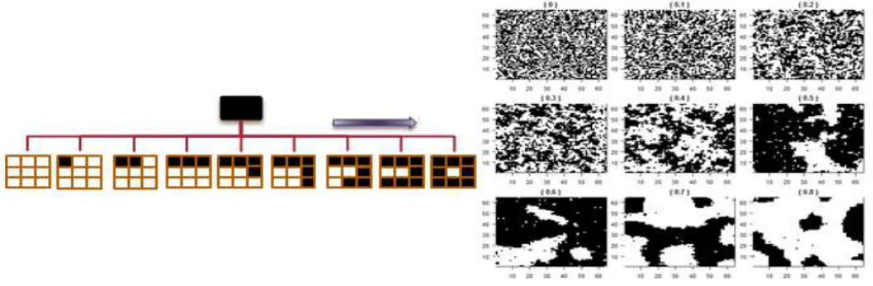
As an example, Figure 6 shows the simulation results for 9 PCT with same tree structure but different transition probabilities. We considered 64×64 sites of a regular lattice and burn-in of 500 and 1000 iterations. The PCN tree used to generate the sample lattice is represented in the left side.
In the right side of Figure 6 each scenario represents a sample generated with a given value of the parameterβ ∈ {0,0.1,0.2,0.3,0.4,0.5}.
3.2. Estimating the PCN
Figure 6: Simulation of Lattices from a Probabilistic Context Neighborhood based on the Ising Model withβ ∈ {0,0.1,0.2,0.3,0.4,0.5}.
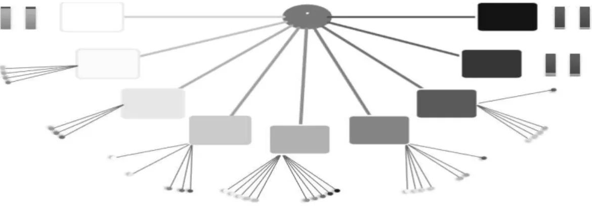
We can observe that our methodology could recover the same neighborhood structure behind the sample (as shown in the right side of the Figure 7). The two bars that appears below each leaf have an area equal to one and represent the conditional probabilities given the observed neighborhoods. The first bar represents the true conditional probability and the second bar represents the estimation of the conditional probability. Thus, the larger the black portion of the bar, the greater the probability of observing a black site i, given the observed neighborhoods. Concluding, the more similar the two bars are, better is the model and closest are the estimates. Thus our methodology has recovered the true model very well.
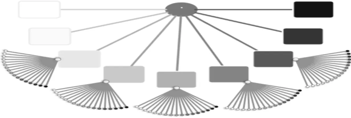
In the second simulation, we generated a sample with 50×50 sites andβ= 0.25. Figure 8 shows the PCN. Due to space limitation, we chose not to draw all context neighborhoods in the PCN of Figure 8. In their place, we created a grey scale that corresponds to the ratio of black in the context neighborhood. Thus, the whiter is the color, the less black sites exist in the context neighborhood. On the contrary, darker the color, the bigger the amount of black sites. Figure 9 shows the scale explained above based on few examples of first and second neighborhoods order.
Figure 8: True NHPCN -order one and two- with conditional probabilities based on the Ising Model andβ = 0.25
Figure 9: Grey scale representing the proportion of black sites in the context neighborhood.
the second-order neighborhood were omitted, but it is important to say that they follow the same trend of the first order.
10
20
30
40
50
10
30
50
Figure 10: Sample obtained in the second order structure.
4. Analysis Via Monte Carlo Simulation
In this section, we are going to analyze the behavior of the estimation method through Monte Carlo Simulation. We generated 100 samples described in section as 3.2 and esti-mated 100 PCN models. The results are exhibited in Table 1. The first column corresponds to context neighborhoods of first order, using values ofs(the number of black sites, minus the number of whites sites). The second and third columns show the true conditional prob-ability and the average estimated conditional probprob-ability in each simulation. Finally, the last column represents the standard deviation of the estimated conditional probabilities.
Figure 11: PCN estimated.
Table 1: Results of simulation
Black-White True probability Estimates S.d
0 0.0180 0.0181 0.0057
1 0.0474 0.0454 0.0185
2 0.1192 0.1235 0.0369
3 0.2689 0.2718 0.0552
4 0.5000 0.4955 0.0517
5 0.7311 0.7359 0.0521
6 0.8808 0.8782 0.0356
7 0.9526 0.9531 0.0177
8 0.9821 0.9813 0.0065
5. Discussion
This tree representation is crucial to understand data interactive behavior.
We are able to calculate for this new model named Probabilistic Context Neighbor-hood the cardinality of the set of context neighborNeighbor-hoods and consequently the number of free parameters because the geometric form of the neighborhoods in this model is fixed. Furthermore we propose an algorithm to estimate the PCN based on the PIC estimator proposed in [23], which uses pseudo-likelihood instead of the likelihood for MRF.
Another contribution of this work is a regionalization scheme based on dissimilarity between Probabilistic Context Neighborhoods. We propose dissimilarity measures that can be more efficient than [28] to capture differences, because it takes into account several characteristics of the PCN’s. In addition to the dissimilarity in probability (commonly used), we also include dissimilarity in structure and complexity. These three dissimilarities are the foundation of our method for regionalization if we consider that the lattice is not homogeneous and have different PCN depending on the sub region. We call this process as Non Homogeneous Probabilistic Context Neighborhood. The regionalization method is based on the SKATER procedure, using the PCN as attributes of each site.
Finally, we tested the method in different scenarios. First, we generated a sample from PCN, evaluating the performance of the method using conditional probabilities based on two dimension Ising Model [29]. Second, we analyze the recovery of a NHPCN with two different neighborhood dependencies in two sub regions with order one and order two PCN. We have found that the estimates were very close to the real source in both cases.
We conclude then that our methodology provides good estimates for PCNs and it is also capable to identify sub regions on a two dimensional lattice.
References
[1] S. Geman, D. Geman, Stochastic relaxation, Gibbs distributions, and the Bayesian restoration of images Pattern Analysis and Machine Intelligence, IEEE Transactions on IEEE 4 (1984) 721-741.
[3] R. Kindermann, J. L. Snell, Markov random fields and their applications, American Mathematical Society Providence RI 1, 1980.
[4] S. K. Kopparapu, U. B. Desai, Bayesian approach to image interpretation, Springer, Powai India, 2001.
[5] S. Z. Li, Markov random field modeling in image analysis, Springer-Verlag London Limited, 2009.
[6] P. L. Dobruschin, The description of a random field by means of conditional proba-bilities and conditions of its regularity, Th. Prob. and Its Appl. 13 (1968) 197-224.
[7] O. Frank, D. Strauss, Markov graphs, Journal of the american Statistical association, Taylor and Francis Group 81 (1986) 832-842.
[8] S. Parise, M. Welling, Structure learning in markov random fields Advances in Neural Information Processing Systems, Citeseer 29 (2006) 54.
[9] J. Rissanen, A universal data compression system Information Theory, Transactions on IEEE 29 (1983) 656-664.
[10] F. Ferrari,A. J. Wyner, Estimation of general stationary processes by variable length markov chains, Scandinavian Journal of Statistics 30 (2003) 459-480.
[11] I. Csisz´ar, P. C. Shields, The consistency of the BIC Markov order estimator, The Annals of Statistics, Institute of Mathematical Statistics 28 (2000) 1601-1619.
[12] I. Csisz´ar, Z. Talata, Context tree estimation for not necessarily finite memory pro-cesses, via BIC and MDL, Information Theory, IEEE Transactions on, IEEE 52 (2006) 1007-1016.
[14] Z. Talata, T. Duncan, Unrestricted BIC context tree estimation for not necessarily finite memory processes Information Theory, ISIT , IEEE International Symposium on, 2009, 724-728.
[15] A. Akimov, A. Kolesnikov, P. Fr¨a nti, Lossless compression of map contours by con-text tree modeling of chain codes, Pattern Recognition, Elsevier 40 (2007) 944-952.
[16] P. B¨uhlmann, Efficient and adaptive post-model-selection estimators, Journal of sta-tistical planning and inference, Elsevier 79 (1999) 1-9.
[17] P. B¨uhlmann, Model selection for variable length Markov chains and tuning the context algorithm, Annals of the Institute of Statistical Mathematics, Springer 52 (2000) 287-315.
[18] A. Garivier, F. Leonardi, Context tree selection: A unifying view, Stochastic Pro-cesses and their Applications, Elsevier 121 (2011) 2488-2506.
[19] G. Bejerano, G. Yona, Variations on probabilistic suffix trees: statistical modeling and prediction of protein families, Bioinformatics, Oxford Univ Press 17 (2001) 23-43.
[20] J. R. Busch, P. A. Ferrari, A. G. Flesia, R. Fraiman, S. P. Grynberg, F. Leonardi, Testing statistical hypothesis on random trees and applications to the protein classi-fication problem, The Annals of Applied Statistics, JSTOR 3 (2009) 542-563.
[21] A. Galves, C. Galves, J. E. Garcia, N. L. Garcia, F. Leonardi, Context tree selection and linguistic rhythm retrieval from written texts, The Annals of Applied Statistics, Institute of Mathematical Statistics 6 (2012) 186-209.
[22] F. M. J. Willems, Y. M. Shtarkov, T. J. Tjalkens, The context-tree weighting method: Basic properties, Information Theory, IEEE Transactions on, IEEE 41 (1995) 653-664.
[24] E. L¨ocherbach, E. Orlandi, Neighborhood radius estimation for variable-neighborhood random fields, Stochastic Processes and their Applications, Elsevier 121 (2011) 2151-2185.
[25] J. P. Lage, R. M. Assun¸c˜ao, E. A. Reis, A minimal spanning tree algorithm applied to spatial cluster analysis, Electronic Notes in Discrete Mathematics, Elsevier 7 (2001) 162-165.
[26] R. M. Assun¸c˜ao, M. C. Neves, G. Cˆamara, C. Da Costa Freitas, Efficient region-alization techniques for socio-economic geographical units using minimum spanning trees, International Journal of Geographical Information Science, Taylor and Francis 20 (2006) 797-811.
[27] M. Bernard, L. Boyer, A. Habrard, M. Sebban, Learning probabilistic models of tree edit distance, Pattern Recognition, Elsevier 41 (2008) 2611-2629.
[28] G. Mazeroff, V. De, C. Jens, G. Michael, G. Thomason, Probabilistic trees and au-tomata for application behavior modeling, 41st ACM Southeast Regional Conference Proceedings, 2003.
[29] R. Peierls, On Isings model of ferromagnetism, Proc. Camb. Phil. Soc 32 (1936) 477-481.
[30] F. M. Willems, Y. M. Shtarkov, T. J. Tjalkens, Context-tree maximizing, Proc., Conf. Information Sciences and Systems, 2000, 7-12.
[31] M. Maravalle, B. Simeone, R. Naldini, Clustering on trees Computational Statistics and Data Analysis, Elsevier 24 (1997) 217-234.
[32] A. V. Aho, J. E. Hopcroft, J. D. Ullman, Estructura de datos y algoritmos, Addison Wesley Iberoamericana, SA Washington. Cap 6 (1988) 200-251.
Vizinhan¸cas a priori em Campos de Markov
Aline Piroutek, Renato Assun¸c˜ao e Denise Duarte
25 de setembro de 2013
Resumo
1
Introdu¸
c˜
ao
O mapeamento de doen¸cas tem sido amplamente usado em an´alises epidemiol´ogicas e nas interven¸c˜oes realizadas no ˆambito da sa´ude p´ublica. Essa ferramenta ´e bastante utilizada para descrever varia¸c˜oes espaciais das taxas de incidˆencias de doen¸cas, identificar ´areas com risco inesperadamente altos e apresentar um mapa de risco de uma regi˜ao permitindo a ado¸c˜ao de pol´ıticas p´ublicas mais eficientes. Uma recente revis˜ao de mapeamento de doen¸cas pode ser visto em [1], [2] e [3], e aplica¸c˜oes em variadas patologias podem ser vistas em [4], [5], [6],[7], [8], [9], [10] e [11].
O modelo mais popular para estimar os riscos relativos foi proposto por Besag, York e Molli´e [12]. Esse modelo tem sido estudado em diversos campos da estat´ıstica, sendo estendido em m´etodos de sobrevivˆencia ([13], [14]), modelos multivariados ( [14], [15], [16], [17]), modelos espa¸co-tempo [18], [19], [20], [21]), entre outros. Em seu trabalho, Besag et al. utiliza a decomposi¸c˜ao do risco relativo em dois efeitos aleat´orios: espacialmente estruturado e espacialmente n˜ao estruturado. O primeiro efeito ´e baseado no modelo conditional autoregressivo (CAR), no qual a dependˆencia espacial ´e expressa atrav´es de uma estrutura Markoviana. Isso significa que o valor do efeito aleat´orio de uma ´area, dado o valor de todas as outras, dependente somente de um conjunto reduzido de ´areas chamado vizinhan¸ca. O segundo efeito assume v.a’s iid normal multivariada. Uma caracter´ıstica desse modelo, assim como da maioria dos modelos focados no mapeamento de doen¸cas, ´e a fixa¸c˜ao de uma estrutura de vizinhan¸cas. Mais especificamente, essa estrutura determin´ıstica ´e expressa atrav´es de uma matriz pouco flex´ıvel e comumente baseada somente em vizinhan¸ca de adjacˆencia. A raz˜ao para esta escolha inclue sua simplicidade, conveniˆencia e f´acil obten¸c˜ao atrav´es de rotinas do GIS (Geographic information system).
Muitos exemplos podem ser levantados apresentando rela¸c˜oes entre a taxa de incidˆencia de uma doen¸ca e fatores n˜ao espaciais ([22], [23],[24] e [25]) , o que torna inadequada a utiliza¸c˜ao apenas da vizinhan¸ca de adjacˆencia.
Em particular, daremos ˆenfase, neste trabalho, `a an´alise dos casos bronquite e bronquilite aguda devido `a cren¸ca na rela¸c˜ao entre taxa de mortalidade e o tamanho da popula¸c˜ao,uma vez que, quanto maior a cidade, maior ´e n´ıvel de polui¸c˜ao do ar ([26],[27] e [28]).
Com o fim de motivar, dividimos as cidades em 4 grupos, e plotamos os box-plots dos logaritmos naturais das taxas de mortalidade. O primeiro grupo, representado no primeiro box-plot da Figura
1, ´e formado pelas microrregi¸coes com o tamanho da popula¸c˜ao pertencente ao primeiro quartil. O segundo grupo, representado no segundo box-plot da Figura 1, ´e constitu´ıdo por microrregi˜oes com popula¸c˜ao pertencente ao segundo quartil, e assim sucessivamente.
1 2 3 4
−11
−10
−9
−8
−7
Figura 1: Box-plots do logaritmo natural das taxas de bronquite e bronquilite aguda. Os grupos 1,2,3 e 4 s˜ao formados pelas microrregi˜oes com a popula¸c˜ao pertecente ao primeiro, segundo, terceiro e quarto quartil, respectivamente.
Analisando os dados, fica f´acil concluir que, quanto maior a popula¸c˜ao da cidade, maior ´e taxa de mortalidade de bronquite e bronquilite agudas.
´
E de se suspeitar que, nesse caso, a vizinhan¸ca baseada na adjacˆencia n˜ao seja uma boa op¸c˜ao. Portanto, seria muito ´util dispor de um modelo que permite que a estrutura de vizinhan¸ca adapta-se automaticamente de acordo com a evidˆencia de dados observado.
De acordo com abordagens em redes bayesianas, aprender a estrutura de um grafo (uma repre-senta¸c˜ao da matriz de vizinhan¸ca) ´e uma tarefa onerosa devido ao grande n´umero de grafos poss´ıveis em um conjunto de n´os (ou vari´aveis). Uma das solu¸c˜oes nesse cen´ario ´e a utiliza¸c˜ao de m´etodos de optimiza¸c˜ao segundo alguma m´etrica ( [29], [30], [31], [32], [33]). Outro tipo de procedimento tem como base a d-separa¸c˜ao (Judea Pearl, [34]), na qual, atrav´es do uso de testes estat´ısticos, as rela¸c˜oes condicionais entre n´os s˜ao identificadas. A partir desse ponto, torna-se indispens´avel o uso de algoritmos baseados na restri¸c˜ao do n´umero de arestas ou vari´aveis.
Ainda nessa linha, podemos citar o trabalho de Born and Caron [35] no qual ´e abordado o problema da aprendizagem estrutural em grafos n˜ao direcionados. Eles utilizam modelos de parti¸c˜ao produto para encontrar clusters a partir de grafos desconexos. Al´em disso, eles prop˜oem uma classe de grafos
a priori baseados no controle de clusteriza¸c˜ao e n´ıvel de separa¸c˜ao do grafo.
No presente trabalho, propomos um modelo de mapeamento de doen¸cas mais flex´ıvel em termos da estrutura de vizinhan¸ca. Nossa maior contribui¸c˜ao est´a nas propostas para as classes de matrizes de vizinhan¸cas a priori. Para permitir ainda mais abrangˆencia, propomos tamb´em a combina¸c˜oes entre elas. Adicionado a esse fato, usamos a abordagem bayesiana e m´etodos computacionais (MCM) para encontrar amostras da matriz de vizinhan¸ca. Por fim, propusemos dois estimadoresa posteriori para as amostras das matrizes permitindo, al´em da estima¸c˜ao do risco relativo, uma an´alise de influˆencia entre ´areas.
2
Mapeamento de doen¸
cas
Considere uma regi˜ao D ⊂ ℜ2. A regi˜ao D ´e um conjunto finito e enumer´avel de s´ıtios geogr´aficos (´areas) D1, D2, . . . , Dn onde D = D1 ∪D2 ∪. . . ,∪Dn com Di∩Dj = ∅ se i ̸= j. Para facilitar a
nota¸c˜ao vamos denotar a regi˜aoDiporicomi= 1, . . . , n. Denotamosyio n´umero observado de casos
na regi˜aoi.
Condicionadas ao vetor de parˆametros ψ, modelamos as contagens como vari´aveis aleat´oias inde-pendentes segundo uma distribui¸c˜ao de Poisson(ψiEi), onde:
Ei = ∑jpopijrj ´e o n´umero esperado de ocorrˆencias na ´area i sob a hip´otese de que risco na
´
areai seja igual ao risco na regi˜ao total
rj = n
∑
i=1
yij n
∑
i=1
popij
´e taxa de incidˆencia da doen¸ca em toda regi˜ao de estudo na faixa et´ariaj para o
sexo feminino/masculino;
popij ´e a popula¸c˜ao em risco da ´area ina faixa et´ariaj.
´
E importante salientar que o risco relativo subjacente ´e representados porψ= (ψ1, . . . , ψn) e, segundo
a abordagem Bayesiana, ser´a considerado como um vetor aleat´orio. Dessa forma, o m´etodo ´e baseado na distribui¸c˜aoa posteriori de ψi:
f(ψ|y)∝l(y1, . . . , yn)f(ψ), (1)
onde l(y1, . . . , yn) ´e a fun¸c˜ao de verossimilhan¸ca e f(ψ) a distribui¸c˜ao a priori do vetor de
parˆametros ψ= (ψ1, . . . , ψn).
A modelagem da distribui¸c˜ao a priori f(ψ) permite introduzir caracter´ısticas dos riscos relativos. A modelagem mais comum ´e feita a partir de um modelo de efeitos aleat´orios, da seguinte maneira:
logψi =µ+ϵi, (2)
em queµrepresenta a m´edia global do risco relativo eϵirepresenta o risco espec´ıfico dai-´esima regi˜ao.
Uma das distribui¸c˜oes mais utilizada nos estudos estat´ısticos foi proposto em Besag et al.(1991) [12] no qual o efeito aleat´orio ϵ´e decomposto em duas componentes, uma n˜ao estruturada espacialmente (φ) e outra estruturada espacialmente (θ):
O primeiro efeito, denotado pela componente φ= (ϕ1, . . . , ϕn), pode decorrer das caracter´ısticas
individuais das ´areas cuja influˆencia se restringe `as fronteiras geogr´aficas e podem ser modeladas como efeitos aleat´orios independentes (por exemplo, a¸c˜oes de sa´ude p´ublica n˜ao compartilhadas entre regi˜oes). Al´em disso, ´e atribu´ıdo ao vetor φuma distribui¸c˜ao conjunta a priori normal multivariada independente, com m´edia 0 e variˆancia 1/τφ. O grau de dispers˜ao dos efeitos aleat´orios n˜ao
estru-turados espacialmente ´e controlado pelo parˆametro desconhecido τφ. Se τφ´e relativamente pequeno,
a variabilidade dos efeitos aleat´orios (ϕ1, . . . , ϕn) ser´a grande em torno de sua m´edia comum igual
a zero, significando grande variabilidade dos riscos relativos. Por outro lado, se τφ ´e relativamente
grande, haver´a uma pequena varia¸c˜ao desses efeitos em torno de zero.
O segundo efeito, representado pela componenteθ= (θ1, . . . , θn), pode ser considerado como efeito
aleat´orio devido `a correla¸c˜ao espacial entre ´areas. Assim, uma ´area tende a ser semelhante `as ´areas vizinhas em termos do risco relativo (por exemplo, ´ındices pluviom´etricos e temperatura em casos de dengue). As componentes desse vetor possuem distribui¸c˜oes condicionais escolhidas como campos aleat´orios de Markov [37] chamado condicional autoregressivo CAR (Besag et al.)[38]:
θi|(θ−i,W, τθ, ρ)∼N
( ρ∑
jwijθj
∑
jwij
, τ
−1
θ
∑
jwij
)
comi= 1, ..., n. (3)
Aqui, ρ∈(0,1) e τθ denota um hiperparˆametro relacionado com a variˆancia de θi dado os valores
dos outros elementos deθ. O elementowij da matrizWrepresenta a estrutura (grau) de dependˆencia
espaciais fixado pelo usu´ario, o que define quais regi˜oes i e j s˜ao vizinhas. A nota¸c˜ao i∼j significa que as ´areas i e j s˜ao vizinhas sendo que wij = 0 quando essas ´areas n˜ao vizinhas. Por conven¸c˜ao,
consideramoswii= 0 para todo i, ou seja, nenhuma regi˜ao ´e vizinha de si mesma. Muitas aplica¸c˜oes
consideram essa estrutura de vizinhan¸ca baseada em adjacˆencia, ondewij = 1 se a regi˜aoj´e adjacente
`a regi˜ao i, ewij = 0 caso contr´ario.
Segundo o Lemma de Brook [39], a densidade conjunta do vetor de parˆametros θ = (θ1, . . . , θn)
toma a forma:
θ|(τθ, W, ρ)∼N(0,(1−ρW∗)−1τθ−1Dτθ), (4)
ondeρ∈(0,1), Dτθ ´e uma matriz diagonal com elementosdii= 1/ni eni =
∑n
j=1wij. No caso do uso da matriz de adjacˆencia, ni representa o n´umero de vizinhos da ´area i. A matriz W∗ representa
a matriz estoc´astica constru´ıda a partir deW, onde w∗
ij =wij/ni.
Como visto na equa¸c˜ao 3, a distribui¸c˜ao dos θ’s depende n˜ao somente de uma estrutura de viz-inhan¸ca espacial mas tamb´em de um parˆametro desconhecido adicional τθ, inversamente relacionado
com a variabilidade de (θ1, . . . , θn).
3
Metodologia
dados. Al´em disso, tamb´em existe a dificuldade ao ter que escolher uma ´unica matriz a ser usada na an´alise com seus parˆametros e caracter´ısticas. Estamos dizendo que essa matriz pode ser considerada um objeto aleat´orio e que temos que trata-lo como tal. Por esse motivo, nossa proposta ´e atribuir `a matriz aleat´oriaW uma classe de distribui¸c˜aoa priori. Dessa forma, atrav´es dos m´etodos Bayesianos, encontraremos as distribui¸c˜oes a posteriori e as distribui¸c˜oes condicionais completas.
3.1 Mapas como Grafos
Os grafos s˜ao estruturas matem´aticas utilizadas para modelar pares de relacionamentos entre objetos de uma certa cole¸c˜ao e podem representar a estrutura de vizinhan¸ca de uma regi˜ao.
Assim, cada ´area ´e um n´o (ou um v´ertice) do grafo, geralmente localizado no centr´oide da ´area. Pares de ´areas com wij >0 s˜ao conectadas por uma aresta. Se wij = 0, nenhuma aresta ´e desenhada.
A largura das arestas ´e proporcional ao valor de wij . Quando a matriz W ´e bin´aria, somente s˜ao
desenhadas as arestas diferentes de zero. Podemos ver na figura 2um exemplo de grafo construido a partir de um mapa no qual somente ligamos ´areas adjacentes (que compartilham fronteira).
Figura 2: Representa¸c˜ao de uma mapa a partir de um grafo.
O mapa em estudo ´e identificado por um grafo G que consiste em dois conjuntosV e E, tamb´em denotado por G = (V, E). O espa¸co de ´ındicesV(G) ´e o conjuto de v´ertices (ou ´areas) de G e E(G) ´e um conjunto de pares n˜ao ordenados de v´ertices deG, chamado de arestas: v´erticesv e v′ s˜ao ligados por uma aresta se e somente se eles s˜ao vizinhos, isto ´e,wvv′ >0.
Um subgrafo de um grafo G ´e um grafo G′ tal que V(G′) ⊆ V(G) e E(G′) ⊆E(G). Um grafo ´e
dito n˜ao direcionado se suas arestas n˜ao tem dire¸c˜ao definida.
Um grafo ´e dito conexo quando existe um caminho (sequˆencia de v´ertices) ligando cada par de v´ertices distintos, caso contr´ario o grafo ´e dito desconexo. Um ciclo ´e um caminho v1,· · ·, vk, vk+1 , ondev1 =vk+1,k≥3. O grafo que n˜ao possui ciclos ´e dito ac´ıclico.
Dado um grafo G conexo e n˜ao direcionado, uma ´arvore geradora T ´e um subgrafo ac´ıclico que conecta todos os v´ertices. Assim, em uma ´arvore, quaisquer dois n´os s˜ao unidos por um ´unico caminho. Al´em disso, o n´umero de arestas ´e igual ao n´umero de n´os menos 1. Isso implica que, se qualquer aresta for apagada, a ´arvore estar´a desmembrada em duas sub´arvores desconectadas. Um ´unico grafo pode formar mais de uma ´arvore geradora.
N´os dizemos que T ´e compat´ıvel com G, se T pode ser obtida a partir da poda de arestas de G. Representamos essa defini¸c˜ao comoT ≺G quandoT ´e compat´ıvel comG e T ̸≺Gcaso contr´ario.
3.2 Classe de distribui¸c˜ao de W
A classe de matrizes W ser´a denotada porW;
A matriz aleat´oria ser´a denotada porW;
Os elementos da matrizW s˜ao representados por Wij;
Seguem alguns exemplos de classes de matrizes que podem ser utilizadas.
1. W1 ={W:W∈ {T :T ≺Wcompleto}},
ondeT representa uma ´arvore geradora do grafo G e Wcompleto representa um grafo completo, no qual todas as ´areas s˜ao vizinhas entre si. N´os dizemos que T) ´e compat´ıvel com Wcompleto, seT pode ser obtida a partir da poda de arestas de Wcompleto. ComoT ´e uma ´avore geradora, devem sem podadas exatamente n(n−1)/2−(n−1) arestas.
O Teorema da Matriz-´arvore, provado por Kirchhoff em 1847 [40], resolveu o problema de de-termina¸c˜ao do n´umero de ´arvores geradoras de um grafo regular.
Duas exemplos de ´arvores geradoras poss´ıvies a partir de um grafo com 20 ´areas pode ser na figura3.
Figura 3: Duas ´avores geradoras poss´ıveis em um grafo com 20 n´os.
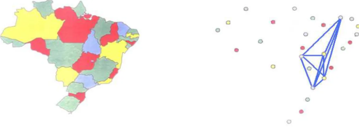
2. W2 ={W(k) :Wij(k) = 1 sej∈ {l:dj(i)≤d(k)(i)}, Wij(k) = 0 c.c.}.
onde dl(i) = ||i−l|| com l ̸= i e d(k)(i) ´e a k-´esima estat´ıstica de ordem. Essa classe cont´em `
aqueles grafos que ligam somente osk∈ {1,2, . . . , n−1}vizinhos mais pr´oximos de cada ´area. A figura4 apresenta exemplos dessa classe em um mapa transformado em grafo no qual variamos os valores dek.
A seguir, apresentamos duas alternativas para distribui¸c˜oes dek :
k∼Ud(1,(n−1)) ,
k= 1 +k∗, com k∗∼Bin(
(n−2), p)
e p∈(0,1),
onde Ud representa a distribui¸c˜ao uniforme discreta. O hiperparˆametro p varia de acordo
Figura 4: Poss´ıveis grafos a partir da classe 2.
3. W3 ={W(d) :Wij(d) = 1 se dj(i)≤d; Wij(d) = 0 c.c.}.
Essa classe tamb´em incorpora um hiperˆametro desconhecido de distˆancia d∈R+ .
A figura5apresenta exemplos dessa classe em um mapa transformado em grafo no qual variamos os valores de d. Observe que, mesmo variando o valor de d entre duas estat´ısticas de ordem consecutivas, o mapa n˜ao se modifica, ou seja, n˜ao ´e acrescentado nenhuma aresta. Dessa forma, o grafo apresenta somente uma aresta quando o valor de d permanece entre d(1)(•) e
d(2)(•). Para que seja acrescentado exatamente uma outra aresta, o valore deddeve se localizar necessariamente no intervalo [d(2)(•), d(3)(•)].
Figura 5: Poss´ıveis grafos a partir da classe 3.
Pode-se, por exemplo, atribuir uma distribui¸c˜ao para o hiperparˆametro dda seguinte forma:
d∼U(d(1)(•), d(n)(•)), ou seja, a distˆancia m´ınima e m´axima entre todos os poss´ıveis pares de v´ertices do grafo.
d=d(n)(•)×d∗, comd∗∼Beta(α, β)
Os hiperparˆametros α e β permitem maior flexibilidade na escolha de d. Se α for igual a um, daremos mais peso para pequenos valores de d. Se tamb´em fixarmos β igual a um, estaremos no caso onde todos os valores poss´ıveis dep tem o mesmo peso.
4. (a) W4 ={W(C) :TAG≺W(C)≺Wadj},
ondeW(C) representa matriz compat´ıvel com Wadj na qual ´e obtida a partir da poda de