Assessment of glacier melt-model transferability: comparison of temperature-index and energy-balance models

(1)

TCD

4, 2143–2167, 2010

Glacier melt-model transferability

A. H. MacDougall et al.

Title Page

Abstract Introduction

Conclusions References

Tables Figures

◭ ◮

Back Close

Full Screen / Esc

Printer-friendly Version Interactive Discussion

Discussion

P

a

per

|

Dis

cussion

P

a

per

|

Discussion

P

a

per

|

Discussio

n

P

a

per

The Cryosphere Discuss., 4, 2143–2167, 2010 www.the-cryosphere-discuss.net/4/2143/2010/ doi:10.5194/tcd-4-2143-2010

The Cryosphere Discussions

This discussion paper is/has been under review for the journal The Cryosphere (TC). Please refer to the corresponding final paper in TC if available.

Assessment of glacier melt-model

transferability: comparison of

temperature-index and energy-balance

models

A. H. MacDougall1, B. A. Wheler1,*, and G. E. Flowers1

1

Department of Earth Sciences, Simon Fraser University, Burnaby, British Columbia, Canada

*

now at: Wek’ `eezh`ıi Land and Water Board, Northwest Territories, Canada

Received: 14 September 2010 – Accepted: 6 October 2010 – Published: 20 October 2010

Correspondence to: G. E. Flowers (gflowers@sfu.ca)

(2)

TCD

4, 2143–2167, 2010

Title Page

Tables Figures

◭ ◮

Back Close

Full Screen / Esc

Discussion

P

a

per

|

Dis

cussion

P

a

per

|

Discussion

P

a

per

|

Discussio

n

P

a

per

|

Abstract

Transferability of glacier melt models is necessary for reliable projections of melt over large glacierized regions and over long time-scales. The transferability of such models has been examined for individual model types, but inter-comparison has been hin-dered by the diversity of validation statistics used to quantify transferability. We apply

5

four common types of melt models – the classical degree-day model, an enhanced temperature-index model, a simplified energy-balance model and a full energy-balance model – to two glaciers in the same small mountain range. The transferability of each model is examined in space and over two melt seasons. We find that the full energy bal-ance model is consistently the most transferable, with deviations in estimated

glacier-10

wide surface ablation of635% when the model is forced with parameters derived from the other glacier and/or melt season. The other three models have deviations in glacier-wide surface ablation of>100% under the same forcings. In addition, we find that there is no simple relationship between model complexity and model transferability.

1 Introduction

15

Climate warming is expected to reduce the extent of the Earth’s mountain glaciers and ice caps during the 21st century, raising eustatic sea level and diminishing fresh water resources (Lemke et al., 2007). Recently there have been attempts to project the mag-nitude of glacier loss using glacier melt models applied over large regions or globally (e.g. de Woul and Hock, 2005; Oerlemans et al., 2005; Raper and Braithwaite, 2006;

20

Schneeberger et al., 2003). Such studies have produced a wide range of projected contributions of mountain glaciers and ice caps to 21st century sea-level rise, from 4 cm Sea Level Equivalent (SLE) (Raper and Braithwaite, 2006) to 36 cm SLE (Bahr et al., 2009), motivating a reexamination of the assumptions necessary to apply these models over large regions. Glacier melt models can be broadly divided into empirical

25

(3)

TCD

4, 2143–2167, 2010

Title Page

Tables Figures

◭ ◮

Back Close

Full Screen / Esc

Discussion

P

a

per

|

Dis

cussion

P

a

per

|

Discussion

P

a

per

|

Discussio

n

P

a

per

use energy-balance theory to solve for the energy available to melt snow or ice (e.g. Hock, 2003, 2005). Although melt-model transferability may not be universally possible (Hock, 2003; Hock et al., 2007), limited mass-balance data make it necessary to apply melt models to large regions without site-specific recalibration.

Several studies have previously investigated the transferability of glacier melt

mod-5

els at regional scales (e.g. Carenzo et al., 2009; MacDougall and Flowers, 2010; Shea et al., 2009). Each of these studies uses a different melt model and each finds certain conditions under which the authors consider the respective model to be transferable. However, direct comparison of previously published studies is complicated by the in-consistency of performance metrics authors use to evaluate model transferability. In an

10

attempt assess the relative transferability of di_fferent model types, we apply the clas-sical temperature-index model (Braun et al., 1993), the enhanced temperature-index model of Hock (1999), a simplified energy-balance model based on that of Oerlemans (2001), and the distributed energy-balance model of MacDougall and Flowers (2010) to two small glaciers in the Donjek Range of the St. Elias Mountains. We conduct

15

a series of experiments to quantify the transferability of each model between our two study glaciers and across the 2008 and 2009 melt seasons. Because of the proximity of our study sites in space and the short duration of our data sets (two seasons), this assessment of transferability should be interpreted as an optimistic one.

1.1 Study site

20

The St. Elias Mountains, located in Northwestern North America, are characterized by extreme topographic gradients (Clarke and Holdsworth, 1984) and host one of the largest glacierized regions outside of the Arctic or Antarctic (Arendt et al., 2008). Dur-ing the latter decades of the 20th century, glaciers in Southeastern Alaska and the Coast Mountains of Northwestern North America contributed more to sea-level rise

25

(4)

TCD

4, 2143–2167, 2010

Title Page

Tables Figures

◭ ◮

Back Close

Full Screen / Esc

Discussion

P

a

per

|

Dis

cussion

P

a

per

|

Discussion

P

a

per

|

Discussio

n

P

a

per

|

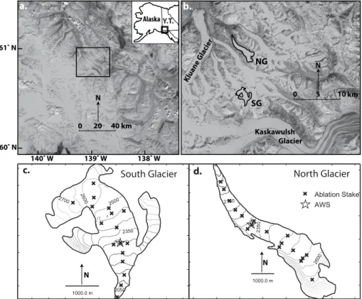
of the St. Elias Mountains in the Southwestern Yukon Territory of Canada (Fig. 1a.). The range is separated from the Gulf of Alaska by less than 100 km, yet experiences a continental climate due to the orographic barriers between the range and the coast (L’Heureux et al., 2004).

This study is conducted on two unnamed mountain glaciers 10 km apart (Fig. 1b).

5

The study glaciers are of similar size and are located on opposing sides of the range crest. One glacier has a predominantly southerly aspect and a surge-type dynamic regime (De Paoli and Flowers, 2009) and is henceforth referred to as “South Glacier” (Fig . 1c). The other has a northwesterly aspect and is referred to as “North Glacier” (Fig. 1d). South Glacier is thought to have a polythermal structure (De Paoli and

Flow-10

ers, 2009) similar to that of Storglaci ¨aren in Northern Sweden (Pettersson et al., 2004). The thermal regime of North Glacier is also presumed to be polythermal but has not been studied. These glaciers were chosen as focussed study sites among the >20 mountain glaciers of the Donjek Range due to their geometric similarities and oppos-ing aspects. The two glaciers have been studied in detail since 2007, with the full

15

complement of instruments required for this study deployed in the 2008 and 2009 field seasons.

2 Methods

2.1 Field methods

2.1.1 Instrumentation and measurements

20

Parallel meteorological and mass-balance measurements were made on each glacier in 2008 and 2009. Automatic weather stations (AWSs) are located in the central ab-lation zones of each glacier at _∼2300 m above sea level (a.s.l.). The AWSs are in-strumented to measure typical meteorological variables, as well as net radiation, and incoming and reflected shortwave radiation (Table 1). An Ultra Sonic Depth Gauge

(5)

TCD

4, 2143–2167, 2010

Title Page

Tables Figures

◭ ◮

Back Close

Full Screen / Esc

Discussion

P

a

per

|

Dis

cussion

P

a

per

|

Discussion

P

a

per

|

Discussio

n

P

a

per

(USDG), which measures surface lowering, is deployed several meters from each AWS. Summer and winter balance is measured at an array of 18 (17) ablation stakes deployed on South (North) Glacier (Fig. 1c,d). Snow-pits are excavated near the AWSs and in the accumulation zones of the glaciers each May, in order to evaluate the density and structure of the snowpack.

5

2.1.2 Data processing

Meteorological data are gap-filled using linear interpolation. No gap in the 2007– 2009 record is longer than 30 min for deployed and undamaged instruments (see Mac-Dougall and Flowers (2010) for details). The USDG record is used to estimate the time and magnitude of snowfall events, and based on measurments fresh snow is assumed

10

to have a density of 200 kg m−3. The ablation stake measurements are used to estimate mass balance following the method of Østrem and Brugman (1991). Initial snow-depth across the glacier is calculated by interpolating measured May snow-depths from the ablation stake locations to all grid points using linear regressions on slope and elevation for South Glacier, and linear regression on elevation for North Glacier (Wheler, 2009;

15

MacDougall, 2010). Snowfall events at the AWS are extrapolated to the rest of the glacier using an empirical precipitation lapse rate (Table 2), a temperature melt/freeze threshold of 1◦C, and the rainfall records from the AWS.

2.2 Modelling methods

Four melt models are used to examine the relationship between model

transferabil-20

ity and model complexity: (1) the Classical Temperature-Index Model (CTIM) (Braun et al., 1993); (2) the Enhanced Temperature-Index Model of Hock (1999) (ETIM); (3) a Simplified Energy-Balance Model based on that of Oerlemans (2001) (SEBM); (4) the Distributed Energy-Balance Model of MacDougall and Flowers (2010) (DEBM). This suite of models is similar to that used by Hock et al. (2007) to inter-compare the

25

(6)

TCD

4, 2143–2167, 2010

Title Page

Tables Figures

◭ ◮

Back Close

Full Screen / Esc

Discussion

P

a

per

|

Dis

cussion

P

a

per

|

Discussion

P

a

per

|

Discussio

n

P

a

per

|

temperature-index model of Pellicciotti et al. (2005) from this study, as it is designed to be tuned with the output of an energy balance model rather than with observations directly. Such tuning would present a methodological inconsistency for the purposes of our model inter-comparison study.

2.2.1 Classical temperature-index model (CTIM)

5

The CTIM is the simplest melt model considered and correlates temperature to melt with an empirical degree-day factor. As for most other implementations of this model, different degree-day factors are used for ice and snow (e.g. Braun et al., 1993). The model takes the form:

M=

DDF_snow_/_iceTa:Ta>0

0 :Ta≤0

(1)

10

where DDFsnow/ice is the degree-day factor for snow or ice. The CTIM is driven with air

temperatureTaand snowfall.

2.2.2 Enhanced temperature-index model (ETIM)

The ETIM is an extension of the classical temperature-index model, where both tem-perature and potential shortwave radiation are correlated to melt. Firn is treated as

15

snow in the model by assigning an arbitrarily deep snow depth above the firn line (Hock, 1999). This model has been widely used and exhibits significant improvements in model skill over the clasical temperature-index approach, with a minimal increase in data requirements (e.g. Hock, 1999; Huss et al., 2008). The model takes the form:

M=

MF+rsnow/iceIp

Ta:Ta>0

0 :Ta≤0

(2)

20

whereM is melt rate, MF is a temperature melt factor, rsnow/ice is the radiation melt

(7)

TCD

4, 2143–2167, 2010

Title Page

Tables Figures

◭ ◮

Back Close

Full Screen / Esc

Discussion

P

a

per

|

Dis

cussion

P

a

per

|

Discussion

P

a

per

|

Discussio

n

P

a

per

space due to the combined effects of the position of the sun and surface slope, surface aspect, and shading from the surrounding topography. The model is driven with air temperature and snowfall.

2.2.3 Simplified energy-balance model (SEBM)

The the simplified energy-balance model of Oerlemans (2001) takes the form:

5

QM=(Sin(1−α))+C0+C1Ta, (3)

where Ta is air temperature, C0 and C1 are empirical factors that together take into

account net longwave radiation and the turbulent heat fluxes. The incoming shortwave radiation (Sin) and albedo (α) are treated in an identical fashion as in the DEBM

de-scribed below. The SEBM differs from the original simplified energy-balance model of

10

Oerlemans (2001) only in its treatment of albedo. The model is driven with air temper-ature, incoming shortwave radiation, and snowfall.

2.2.4 Distributed energy-balance melt model (DEBM)

Energy-balance models parameterize or utilize measurements of all of the components of the surface energy balance of ice or snow to solve for the energy available for melt as

15

a residual. Distributed energy-balance models extrapolate the surface energy balance across a grid on the glacier surface. A full description of the DEBM and model validation is given in MacDougall and Flowers (2010). A brief description of the model is recalled below.

The energy balance is written as:

20

QM=(Sin(1−α)+Lin−Lout)+QH+QL−Qg, (4)

(8)

TCD

4, 2143–2167, 2010

Title Page

Tables Figures

◭ ◮

Back Close

Full Screen / Esc

Discussion

P

a

per

|

Dis

cussion

P

a

per

|

Discussion

P

a

per

|

Discussio

n

P

a

per

|

is the sensible heat flux, the energy exchanged between the glacier and the atmo-sphere. QL is the latent heat flux, the heat transferred to or from the glacier through

sublimation, deposition, evaporation or condensation.Qgis the heat transferred to and

from the glacier subsurface when the subsurface changes temperature. QMis the

en-ergy available to melt ice or snow. The sensible heat flux from rain was found to be

5

negligible and is therefore disregarded.

To extrapolate measured incoming shortwave radiation (Sin) to each grid point,Sinis

broken into direct and di_ffuse components following Collares-Pereira and Rabl (1979) and Hock and Holmgren (2005). Direct shortwave radiation is only incident on the frac-tion of the glacier unshaded by surrounded terrain, while diffuse radiation is assumed

10

to originate from all parts of the sky equally and is therefore applied to all grid cells. If the AWS is shaded by surrounding topography all measured incoming shortwave radi-ation is diffuse (Hock and Holmgren, 2005); in this situation the ratio of direct to diffuse shortwave radiation from the most recent time where the AWS was unshaded is used to approximate direct shortwave radiation at unshaded grid cells.

15

Albedo (α), is parameterized following Hock and Holmgren (2005):

αt=

  

 

αt₋1−a1(ln(Ta+1))e(

a₂√n_d_{) if}

nd>0 and Ta>0 αt₋1−a3e(

a₂√n_d₎

if nd>0 and Ta<0 αt−1+a4Ps if nd=0

(5)

whereαt₋1is the albedo at the previous time step, αt is the albedo at the current time

step,ndis the number of days since the last snow fall,Psis the measured rate of snow

fall,Tais air temperature anda1:4are constants that must be found through calibration

20

(Hock and Holmgren, 2005). A constant elevation firn-line was assigned based on field observations (Table 2). Ice is assumed to have a constant albedo (e.g. Hock and Holmgren, 2005; Oerlemans and Knap, 1998).

Outgoing longwave radiation (Lout) is calculated from the temperature of the ice or

snow surface (Ts) according to the Stefan-Boltzmann relationship. The surface

temper-25

(9)

TCD

4, 2143–2167, 2010

Title Page

Tables Figures

◭ ◮

Back Close

Full Screen / Esc

Discussion

P

a

per

|

Dis

cussion

P

a

per

|

Discussion

P

a

per

|

Discussio

n

P

a

per

scheme, in whichQgis taken as the residual of the energy balance when it is negative.

The subsurface flux is then forced into a thin subsurface layer such that

△Ts= Qg ρscsh△

t, (6)

where△t is the model time-step in seconds,ρs is the surface material density, cs is

the specific heat capacity of ice, and his the thickness of the subsurface layer. This

5

subsurface scheme is a compromise between a more complicated multi-layer subsur-face model and simpler constant temperature or iterative approximations. The scheme allows for temporary heat storage in the subsurface with minimal data requirements (Wheler and Flowers, 2010). Incoming longwave radiation (Lin) is computed as the

residual of the radiative energy balance at the AWS location and is assumed to be

10

constant over the entire glacier, following Hock and Holmgren (2005).

Sensible (QH) and latent heat fluxes (QL) are calculated using the bulk aerodynamic

approach as in other recent DEBM studies (e.g. Anderson et al., 2010; Anslow et al., 2008; Brock et al., 2000; Hock and Holmgren, 2005). The aerodynamic roughness-length (zo) used in the bulk aerodynamic approach is estimated using the snow aero-15

dynamic roughness length evolution parameterization of Brock et al. (2006):

ln(zo)=b1

arctan

₍_P

dd−b2) b3

−b4, (7)

wherePdd is the base 10 logarithm of the sum of daily maximum temperatures since

the last snow fall event andb1:4are empirical constants. We use the mean value of the

measured roughness of ice for each glacier. Firn is treated simply as very old snow

20

by settingPdd to be arbitrarily large. The DEBM is driven by air temperature, incoming

(10)

TCD

4, 2143–2167, 2010

Title Page

Tables Figures

◭ ◮

Back Close

Full Screen / Esc

Discussion

P

a

per

|

Dis

cussion

P

a

per

|

Discussion

P

a

per

|

Discussio

n

P

a

per

|

2.2.5 Model calibration and tuning

The three models with empirical melt factors (CTIM, ETIM and SEBM) are tuned by minimizing the root mean square error (RMSE) between measured and modelled ab-lation at the stake locations. The DEBM is calibrated using the record of albedo at the AWSs to solve for albedo parameters separately for each glacier and for each summer.

5

The snow roughness-length evolution parameters are calibrated to roughness-length measurements that were taken only in the summer of 2009. The roughness-length measurements from both glaciers were used together for the calibration, as insu_ffi -cient data exist to calibrate independently for each glacier. The mass-balance data are not used to calibrate the DEBM. See MacDougall and Flowers (2010) for details. The

10

albedo parameterization for the SEBM is calibrated in an identical fashion to that for the DEBM.

2.3 Model transferability experiment design

To evaluate relative model skill, control runs were performed in which each model was run for each glacier and year using locally derived parameter values. Control runs are

15

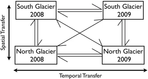
also used a reference against which to evaluate the results of the transferability tests. Model transferability is the ability of a model calibrated for one time and location to produce realistic results for another time and/or location. Here we describe transferabil-ity in terms of model parameter values: that is, the abiltransferabil-ity of parameters calibrated for one time or location to describe another. We assess parameter transferability in time,

20

in space and in space and time together for each model (Fig. 2). In each of these tests the parameter values derived for one glacier and year are used in place of those locally derived for the other glacier and/or year. We use the RMSE between the simulated and the measured cumulative ablation at the stake locations to evaluate the success of the model transfer. An additional experiment is carried out to test the robustness of the

25

(11)

TCD

4, 2143–2167, 2010

Title Page

Tables Figures

◭ ◮

Back Close

Full Screen / Esc

Discussion

P

a

per

|

Dis

cussion

P

a

per

|

Discussion

P

a

per

|

Discussio

n

P

a

per

3 Results

3.1 Comparison to ablation stakes

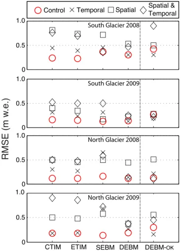
The RMSE values for the control runs relative to the ablation stake measurements are shown in Fig. 3 for each model and data set (symbol). For both glaciers the model with the highest model skill is the ETIM for the 2008 simulations and the SEBM for the

5

2009 simulations. The lowest model skill is achieved by the SEBM for both glaciers in 2008, the CTIM for South Glacier 2009, and the DEBM for North Glacier 2009.

In 11 of 16 temporal transferability tests (×symbol in Fig. 3) the results more closely resemble the control runs than do those of any of the other transferability tests. This is particularly true for the DEBM (see DEBM in Fig. 3), where all of the temporal

trans-10

ferability tests are close to the control run, though untrue for the SEBM where none of the temporal transferability tests are closest to the control. There is a high variability in the results from spatial and spatial-temporal model transfer tests ( and♦symbols,

respectively in Fig. 3) but these transfers frequently produce much larger errors than the control runs.

15

The comparison between model results in Fig. 3 demonstrates that the DEBM is the most transferable of the models considered, as assessed by the spread of transferabil-ity test results. The SEBM is the second most transferable model for the North Glacier 2009 experiments, yet the least transferable for the North Glacier 2008 experiment. The ETIM performs better than the CTIM, but more poorly than the DEBM in each

ex-20

periment. The only exceptions to the DEBM exhibiting the highest transferability are: the spatial transfer on North Glacier in 2008, where all of the models achieve similar RMSEs, the spatial-temporal transfer on South Glacier in 2008 where the SEBM per-forms best, and the spatial transfer on South Glacier in 2009 where the SEBM perper-forms better than all of the other models.

(12)

TCD

4, 2143–2167, 2010

Title Page

Tables Figures

◭ ◮

Back Close

Full Screen / Esc

Discussion

P

a

per

|

Dis

cussion

P

a

per

|

Discussion

P

a

per

|

Discussio

n

P

a

per

|

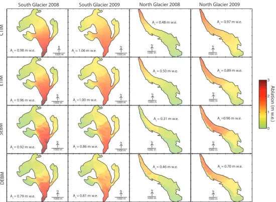
3.2 Comparison between control runs

Glacier melt models are typically applied beyond the stake locations to estimate surface ablation for an entire glacierized basin. Such estimates are shown for each of the control runs in Fig. 4. The spatial patterns of surface ablation in Fig. 4 testify to the increasing complexity of model output with increasing model sophistication. The more

5

complex models estimate higher glacier-wide surface ablation (A_s) than the simpler models. The difference between the highest and lowest estimates ofAsfor each glacier

and year are considerable, ranging between 24% and 41% of the value ofAsestimated

by the DEBM. This large variability is disconcerting, as each of these modelled values of ablation can justifiably be considered a valid estimate.

10

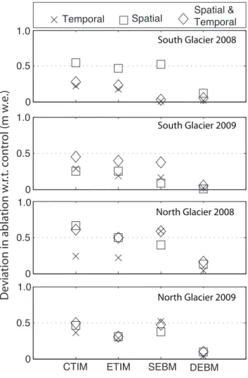
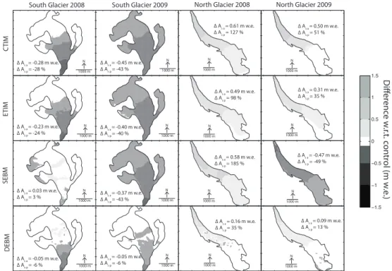
3.3 Comparison of transfer experiments to control runs

The absolute deviations between values ofAs estimated in each transfer test and

es-timated in the control run for a given model (Fig. 5) clearly demonstrate that only the DEBM transfer tests consistently produce estimated ablation anywhere close to the control run. The greatest deviation for the CTIM is 0.66 m w.e. (137% relative to control

15

runAs), for the ETIM 0.50 m w.e. (100%), for the SEBM 0.58 m w.e. (185%), and for

the DEBM 0.16 m w.e. (35%). The spatial distributions of the di_fference in estimated surface ablation between the control run and each spatial-temporal transferability test for a given model are shown in Fig. 6. This figure demonstrates that the differences are proportional to the magnitude of ablation for the empirical models (CTIM and ETIM),

20

(13)

TCD

4, 2143–2167, 2010

Title Page

Tables Figures

◭ ◮

Back Close

Full Screen / Esc

Discussion

P

a

per

|

Dis

cussion

P

a

per

|

Discussion

P

a

per

|

Discussio

n

P

a

per

4 Discussion

The outcome that a physically-based glacier melt model is more transferable than em-pirical models is not a surprise (Hock, 2005). A model that better describes a physical system is expected to be more transferable than one that lumps site-specific properties and weather conditions together (Hock, 2005). This intuitive result has however, to our

5

knowledge, not been previously demonstrated beyond a single glacier study site. An intriguing outcome of these experiments is that, aside from the DEBM being more transferable than the other models, there is no simple relationship between model com-plexity and transferability. The relatively low transferability of the SEBM is surprising considering that the highest model sensitivity in the DEBM comes from the albedo

pa-10

rameterization (MacDougall and Flowers, 2010), which is treated in an identical fashion in the SEBM. This suggests that the SEBM’s transferability is affected by the model’s treatment of the turbulent and longwave heat fluxes, despite these fluxes generally being of secondary importance in our study area (MacDougall and Flowers, 2010).

Unlike the other models considered here, the DEBM has many subcomponents that

15

may differ from those found in other full energy balance models (Brock et al., 2000; Anslow et al., 2008; Hock and Holmgren, 2005; Anderson et al., 2010, e.g.). It is therefore valid to ask whether the high model transferability found in these experiments is unique to the DEBM or its application here, rather than being a general result for all energy balance models of similar or greater complexity. To investigate this question

20

the most sensitive component of the DEBM, the albedo evolution parameterization, was substituted and the transferability experiments repeated. The substitute albedo parameterization was that of Oerlemans and Knap (1998) which relates the albedo of snow to the snow depth and the time elapsed since the last snowfall. Firn and ice have constant albedos. The results of these tests (Fig. 3, DEBM-OK) demonstrate, with

25

(14)

TCD

4, 2143–2167, 2010

Title Page

Tables Figures

◭ ◮

Back Close

Full Screen / Esc

Discussion

P

a

per

|

Dis

cussion

P

a

per

|

Discussion

P

a

per

|

Discussio

n

P

a

per

|

choice of parameterizations is still important as results do not always follow the general pattern expected of the models.

5 Conclusions

We examined the transferability in space and time of four commonly used types of glacier melt models applied to two small glaciers in the St. Elias Mountains of

North-5

western Canada. Our results demonstrate that the physically-based energy-balance model is the most transferable model in space and time, exhibiting635% variation in estimated glacier-wide surface ablation when using model parameters calibrated for a di_fferent melt season and/or another nearby glacier. Under the same conditions, the other models produced variations in estimated glacier-wide surface ablation exceeding

10

100%. No simple relationship between model complexity and model transferability is observed. Deviations in estimated glacier-wide surface ablation between the models in the control runs themselves were 24–41%. These results suggest that physically-based models should be the first choice when applying a glacier melt model over large regions. If insu_fficient data exist to implement such models, enhanced

temperature-15

index models appear to be the next most appropriate choice. There is a need for similar experiments to be conducted in other glacierized regions and over longer time scales for a general confirmation of the conclusions presented here.

Acknowledgements. We are grateful to the Natural Science and Engineering Research Council

of Canada (NSERC), the Canada Foundation of Innovation (CFI), the Canada Research Chairs

20

(CRC) program, the Northern Scientific Training Program (NSTP), and Simon Fraser University for funding. AHMD is grateful for his support from NSERC PGS-M. Permission to conduct this research was granted by the Kluane First Nation, Parks Canada, and the Yukon Territorial Government. Support from the Kluane Lake Research Station (KLRS) and Kluane National Park and Reserve is greatly appreciated. We are indebted to Andy Williams, Sian Williams,

25

(15)

TCD

4, 2143–2167, 2010

Title Page

Tables Figures

◭ ◮

Back Close

Full Screen / Esc

Discussion

P

a

per

|

Dis

cussion

P

a

per

|

Discussion

P

a

per

|

Discussio

n

P

a

per

References

Anderson, B., MacKintosh, A., Stumm, D., George, L., Kerr, T., Winter-Billington, A., and Fitz-simons, S.: Climate sensitivity of a high-precipitation glacier in New Zealand, J. Glaciol., 56, 114–128, 2010. 2151, 2155

Anslow, F., Hostetler, S., Bidlake, W. R., and Clark, P. U.: Distributed energy balance modelling

5

of South Cascade Glacier, Washington and assessment of model uncertainty, J. Geophys. Res., 113, doi:10.1029/2007JF000850, 2008. 2151, 2155

Arendt, A., Luthcke, S., Larsen, C., Abdalati, W., Krabill, W., and Beedle, M.: Validation of high-resolution GRACE mascon estimates of glacier mass changes in the St. Elias Mountains, Alaska, USA, using aircraft laser altimetry, J. Glaciol., 256, 165–172, 2008. 2145

10

Bahr, D., Dyurgerov, M., and Meier, M.: Sea-level rise from glaciers and ice caps: a lower bound, Geophys. Res. Lett., 36, doi:10.1029/2008GL036309, 2009. 2144

Berthier, E., Schiefer, E., Clarke, G., Menounos, B., and R ´emy, F.: Contribution of Alaskan glaciers to sea-level rise derived from satellite imagery, Nat. Geosci., 3(2), 92–95, doi:10.1038/NGEO737, 2010. 2145

15

Braun, L., Grabs, W., and Rana, B.: Application of a conceptual precipitation-runo_ffmodel in the Langtang Khola Basin, Nepal Himalaya, in: Snow and Glacier Hydrology, Proceedings of the Kathmandu Symposium 1992, edited by: Young, G., 221–237, IAHS, Wallingford, England OX10 8BB, 1993. 2145, 2147, 2148

Brock, B., Willis, I., and Sharp, M. J.: Measurement and parameterization of albedo

20

variations at Haut Glacier d’Arolla, Switzerland, J. Glaciol., 46, 657–688, doi:10.3189/ 172756500781832675, 2000. 2151, 2155

Brock, B., Willis, I. C., and Sharp, M. J.: Measurement and parameterization of aerodynamic roughness length at Haut Glacier d’Arolla, Switzerland, J. Glaciol., 52, 281–297, 2006. 2151 Carenzo, M., Pellicciotti, F., Rimkus, S., and Burlando, P.: Assessing the transferability and

25

robustness of an enhanced temperature-index glacier-melt model, J. Glaciol., 55, 258–274, 2009. 2145

Clarke, G. and Holdsworth, G.: Glaciers of the St. Elias Mountains, US Geological Survey professional paper, Washington, DC, USA, ISSN 1044-9612, 1984. 2145

Collares-Pereira, M. and Rabl, A.: The average distribution of solar radiation: correlations

be-30

tween daily and hourly insolation values, Sol. Energy, 22, 155–164, 1979. 2150

(16)

TCD

4, 2143–2167, 2010

Title Page

Tables Figures

◭ ◮

Back Close

Full Screen / Esc

Discussion

P

a

per

|

Dis

cussion

P

a

per

|

Discussion

P

a

per

|

Discussio

n

P

a

per

|

geophysical inversion, J. Glaciol., 55, 1101–1112, 2009. 2146

de Woul, M. and Hock, R.: Static mass-balance sensitivity of Arctic glaciers and ice caps using a degree day approach, Ann. Glaciol., 42, 217–224, 2005. 2144

Hock, R.: A distributed temperature-index ice- and snowmelt model including potential direct solar radiation, J. Glaciol., 45(149), 101–111, 1999. 2145, 2147, 2148

5

Hock, R.: Temperature index melt modelling in mountain areas, J. Hydrol., 282, 104–115, 2003. 2145

Hock, R.: Glacier melt: a review of processes and their modelling, Prog. Phys. Geog., 29(3), 362–391, 2005. 2145, 2155

Hock, R. and Holmgren, B.: A distributed energy-balance model for complex topography

10

and its application to Storglaci ¨aren, Sweden, J. Glaciol., 51, 25–36, doi:10.3189/ 172756505781829566, 2005. 2150, 2151, 2155

Hock, R., Radi´c, V., and de Woul, M.: Climate sensitivity of Storglaci ¨aren, Sweden: an inter-comparison of mass-balance models using ERA-40 re-analysis and regional climate model data, Ann. Glaciol., 46, 342–348, 2007. 2145, 2147

15

Huss, M., Farinotti, D., Bauder, A., and Funk, M.: Modelling runofffrom highly glacierized alpine drainage basins in a changing climate, Hydrol. Process., 22, 3888–3902, 2008. 2148 Kaser, G., Cogley, J., Dyurgerov, M., Meier, M., and Ohmura, A.: Mass balance of glaciers

and ice caps: Consensus estimates for 1961–2004, Geophys. Res. Lett., 33, doi:10.1029/ 2006GL027511, 2006. 2145

20

Lemke, P., Ren, J., Alley, R., Allison, I., Carrasco, J., Flato, G., Fujii, Y., Kaser, G., Mote, P., Thomas, R., and Zhang, T.: Observations: changes in snow, ice and frozen ground, in: Climate Change 2007: The Physical Science Basis. Contribution of Working Group I to the Fourth Assessment Report of the Intergovernmental Panel on Climate Change, edited by: Solomon, S., Qin, D., Manning, M., Chen, Z., Marquis, M., Averyt, K., Tignor, M., and

25

Miller, H., Cambridge University Press, Washington, DC, USA, 2007. 2144, 2145

L’Heureux, M., Mann, M., Cook, B., Gleason, B., and Voss, R.: Atmospheric circulation influ-ences on seasonal precipitation patterns in Alaska during the latter 20th century, J. Geophys. Res., 109, doi:10.1029/2003JD003845, 2004. 2146

MacDougall, A.: Distributed energy-balance glacier melt-modelling in the Donjek Range of

30

(17)

TCD

4, 2143–2167, 2010

Title Page

Tables Figures

◭ ◮

Back Close

Full Screen / Esc

Discussion

P

a

per

|

Dis

cussion

P

a

per

|

Discussion

P

a

per

|

Discussio

n

P

a

per

MacDougall, A. and Flowers, G.: Spatial and temporal transferability of a distributed energy-blance glacier melt-model, submitted, J. Climate, 2010. 2145, 2147, 2149, 2152, 2155 Oerlemans, J.: Glaciers and Climate Change, 1st edn., Swets and Zeitlinger BV, Lisse, 2001.

2145, 2147, 2149

Oerlemans, J. and Knap, W. H.: A one year record of global radiation and albedo in the ablation

5

zone of Morteratschgletscher, Switzerland,, J. Glaciol., 44, 231–238, 1998. 2150, 2152, 2155, 2164

Oerlemans, J., Bassford, R., Chapman, W., Dowdeswell, J., Glazovsky, A., Hagen, J., Melvold, K., de Ruyter de Wildt, M., and van de Wal, R.: Estimating the contribution of Arctic glaciers to sea-level change in the next 100 years, Ann. Glaciol., 42, 230–236, 2005.

10

2144

Østrem, G. and Brugman, M.: Glacier mass-balance measurements: a manual for field and o_ffice work, National Hydrology Research Institute, Saskatoon Canada, 1991. 2147

Pellicciotti, F., Brock, B., Strasser, U., Burlando, P., Funk, M., and Corripio, J.: An enhanced temperature-index glacier melt model including the shortwave radiation balance:

develop-15

ment and testing for Haut Glacier d’Arolla, Switzerland, J. Glaciol., 51, 573–587, 2005. 2148 Pettersson, R., Jansson, P., and Blatter, H.: Spatial variability in water content at the cold– temperate transition surface of the polythermal Storglaci ¨aren, Sweden, J. Geophys. Res., 109, doi:10.1029/2003JF000110, 2004. 2146

Raper, S. and Braithwaite, R.: Low sea level rise projections from mountain glaciers and

ice-20

caps under global warming, Nature, 439, 311–313, 2006. 2144

Schneeberger, C., Blatter, H., Abe-Ouchi, A., and Wild, M.: Modelling changes in the mass balance of glaciers of the Northern Hemisphere for a transient 2_×CO₂scenario, J. Hydrol., 282, 145–263, 2003. 2144

Shea, J., Moore, R., and Stahl, K.: Derivation of melt factors from glacier mass-balance records

25

in Western Canada, J. Glaciol., 55, 123–130, 2009. 2145

Wheler, B.: Glacier melt modelling in the Donjek Range, St. Elias Mountains, Yukon Territory, Master’s thesis, Simon Fraser University, Burnaby, British Columbia, Canada, 2009. 2147 Wheler, B. and Flowers, G.: Glacier subsurface heat-flux characterizations for energy balance

modelling in the Donjek Range, Southwest Yukon Territory, Canada, accepted, J. Glaciol.,

30

(18)

TCD

4, 2143–2167, 2010

Title Page

Tables Figures

◭ ◮

Back Close

Full Screen / Esc

Discussion

P

a

per

|

Dis

cussion

P

a

per

|

Discussion

P

a

per

|

Discussio

n

P

a

per

|

Table 1. Instrumentation deployed at AWS locations on North Glacier and South Glacier. In-strument precision is taken from manufacturer’s documentation. Rainfall for South Glacier was measured 500 m from AWS.

Variable Instrument Precision

(19)

TCD

4, 2143–2167, 2010

Title Page

Tables Figures

◭ ◮

Back Close

Full Screen / Esc

Discussion

P

a

per

|

Dis

cussion

P

a

per

|

Discussion

P

a

per

|

Discussio

n

P

a

per

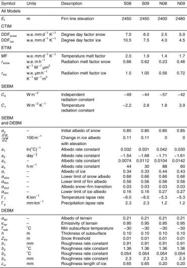
Table 2.Parameters used in each of the four melt models. S08 is South Glacier 2008, S09 is South Glacier 2009, N08 is North Glacier 2008 and N09 is North Glacier 2009.

Symbol Units Description S08 S09 N08 N09 All Models

E_f m Firn line elevation 2450 2450 2400 2480 CTIM

DDFsnow w.e. mm d−1K−1 Degree day factor snow 7.0 6.0 2.5 5.0

DDFice w.e. mm d−1K−1 Degree day factor ice 10.5 7.5 4.0 4.5

ETIM

MF w.e. mm d−1_K−1 _{Temperature melt factor} _2.0 _1.9 _1.4 _1.7

rsnow w.e. m h−1 Radiation melt factor snow 0.66 0.62 0.23 0.46

K−1W−1µm2

rice w.e. µm h−1 Radiation melt factor ice 1.5 1.05 0.56 0.72

K−1_W−1_m2

SEBM

C₀ W m−2

Independent −49 −44 −57 −42 radiation constant

C1 W m−2K−1 Temperature −2.2 2.8 1.8 3.9

radiation constant SEBM

and DEBM

αo – Initial albedo of snow 0.85 0.85 0.85 0.85

d αi

dZ 100 m−

1

Change in ice albedo 0.11 0.11 0 0 with elevation

a₁ ln(◦_C)−1 _{Albedo rate constant} _0.032 _0.031 _0.042 _0.030

a2 day−

1

2 _{Albedo rate constant} ₋_1.54 ₋_1.68 ₋_1.71 ₋_1.61

a3 – Albedo rate constant 0.0074 0.0112 0.0104 0.0142

a₄ h m−1 Albedo rate constant 44 30 88 60

α_i – Albedo of ice 0.34 0.33 0.44 0.43

α_slim – Lower limit of snow albedo 0.66 0.66 0.66 0.66

α_flim – Lower limit of firn albedo 0.56 0.56 0.56 0.56

α_stof – Albedo snow–firn transition 0.03 0.03 0.03 0.03

αilim – Lower limit of ice albedo 0.16 0.16 0.27 0.27

ΓT K km−1 Temperature lapse rate −6.0 −6.0 −5.3 −5.3

Γp mm km−1 Precipitation lapse rate 2.3 2.3 1.2 1.2

DEBM

α_ter – Albedo of terrain 0.21 0.21 0.21 0.21

ǫ_ter – Emissivity of terrain 0.95 0.95 0.95 0.95

T_sub ◦_C _{Min subsurface temperature} ₋₃₀ ₋₃₀ ₋₃₀ ₋₃₀

h m Thickness of subsurface 0.10 0.10 0.10 0.10

Zthr m Snow threshold 0.01 0.01 0.01 0.01

b1 mm Roughness rate constant 0.91 0.91 0.91 0.91

b2 ◦C Roughness rate constant 1.36 1.36 1.36 1.36

b3 ◦C Roughness rate constant 0.054 0.054 0.054 0.054

b4 mm Roughness rate constant 2.3 2.3 2.3 2.3

(20)

TCD

4, 2143–2167, 2010

Title Page

Tables Figures

◭ ◮

Back Close

Full Screen / Esc

Discussion

P

a

per

|

Dis

cussion

P

a

per

|

Discussion

P

a

per

|

Discussio

n

P

a

per

|

SG NG

0 5 10

N

km

Kaskawulsh Glacier

Kluane Glacier

0 20 40 km

N

139˚ W 138˚ W

140˚ W 60˚ N

61˚ N

b. a.

Alaska

2050

2350

2500

2600 2700

1000.0 m

2350

2600

2150

1000.0 m

Ablation Stake

AWS

c. d.

N

South Glacier North Glacier

Y.T.

(21)

TCD

4, 2143–2167, 2010

Title Page

Tables Figures

◭ ◮

Back Close

Full Screen / Esc

Discussion

P

a

per

|

Dis

cussion

P

a

per

|

Discussion

P

a

per

|

Discussio

n

P

a

per

South Glacier

2008

South Glacier

2009

North Glacier

2008

North Glacier

2009

Temporal Transfer

Spatial

Transf

er

(22)

TCD

4, 2143–2167, 2010

Title Page

Tables Figures

◭ ◮

Back Close

Full Screen / Esc

Discussion

P

a

per

|

Dis

cussion

P

a

per

|

Discussion

P

a

per

|

Discussio

n

P

a

per

|

0 0.5 1.0

Control Temporal Spatial Spatial & _Temporal

0 0.5 1.0

CTIM ETIM SEBM DEBM DEBM-OK

RMSE (m w

.e.)

South Glacier 2008

South Glacier 2009

North Glacier 2008

North Glacier 2009

(23)

TCD

4, 2143–2167, 2010

Title Page Abstract Introduction Conclusions References Tables Figures ◭ ◮ ◭ ◮ Back Close

Full Screen / Esc

Printer-friendly Version Interactive Discussion Discussion P a per | Dis cussion P a per | Discussion P a per | Discussio n P a per

South Glacier 2008 South Glacier 2009 North Glacier 2008 North Glacier 2009

C TIM E TIM SEBM DEBM 0 1 2 3 A bla

tion (m w

.e .) N 1000 m N 1000 m N 1000 m N 1000 m N 1000 m N 1000 m N 1000 m N 1000 m N 1000 m N 1000 m N 1000 m N 1000 m N 1000 m N 1000 m N 1000 m N 1000 m A

s = 0.98 m w.e.

A

s = 0.96 m w.e.

A

s = 0.92 m w.e.

A

s = 0.79 m w.e.

As = 1.06 m w.e.

A

s =1.00 m w.e.

A

s = 0.86 m w.e.

A

s = 0.81 m w.e.

A

s = 0.48 m w.e.

A

s = 0.50 m w.e.

A

s = 0.31 m w.e.

A

s = 0.46 m w.e.

A

s = 0.97 m w.e.

A

s = 0.89 m w.e.

A

s =0.96 m w.e.

A

s = 0.70 m w.e.

(24)

TCD

4, 2143–2167, 2010

Title Page

Tables Figures

◭ ◮

Back Close

Full Screen / Esc

Discussion

P

a

per

|

Dis

cussion

P

a

per

|

Discussion

P

a

per

|

Discussio

n

P

a

per

|

0 0.5 1.0

CTIM ETIM SEBM DEBM

0 0.5 1.0

Temporal Spatial Spatial & _Temporal

D

evia

tion in abla

tion w

.r

.t

. c

on

tr

ol (m w

.e

.)

South Glacier 2008

South Glacier 2009

North Glacier 2008

North Glacier 2009

(25)

TCD

4, 2143–2167, 2010

Title Page Abstract Introduction Conclusions References Tables Figures ◭ ◮ ◭ ◮ Back Close

Full Screen / Esc

Printer-friendly Version Interactive Discussion Discussion P a per | Dis cussion P a per | Discussion P a per | Discussio n P a per −1.5 −1 −0.5 0 0.5 1 1.5 South Glacier 2008 South Glacier 2009 North Glacier 2008 North Glacier 2009

C TIM E TIM SEBM DEBM Diff er enc e w .r .t . c on tr

ol (m w

.e .) N 1000 m N 1000 m N 1000 m N 1000 m N 1000 m N 1000 m N 1000 m N 1000 m N 1000 m N 1000 m N 1000 m N 1000 m N 1000 m N 1000 m N 1000 m N 1000 m

∆ As a = -0.28 m w.e.

∆ As p = -28 %

∆ As a = -0.23 m w.e.

∆ As p = -24 %

∆ As a = 0.03 m w.e.

∆ As p = 3 %

∆ As a = -0.05 m w.e.

∆ As p = -6 %

∆ As a = -0.45 m w.e.