TCD
5, 2115–2157, 2011The mass balance gradient method
M. M. Helsen et al.
Title Page
Abstract Introduction
Conclusions References
Tables Figures
◭ ◮
◭ ◮
Back Close
Full Screen / Esc
Printer-friendly Version Interactive Discussion
Discussion
P
a
per
|
Dis
cussion
P
a
per
|
Discussion
P
a
per
|
Discussio
n
P
a
per
|
The Cryosphere Discuss., 5, 2115–2157, 2011 www.the-cryosphere-discuss.net/5/2115/2011/ doi:10.5194/tcd-5-2115-2011
© Author(s) 2011. CC Attribution 3.0 License.
The Cryosphere Discussions
This discussion paper is/has been under review for the journal The Cryosphere (TC). Please refer to the corresponding final paper in TC if available.
Towards direct coupling of regional
climate models and ice sheet models by
mass balance gradients: application to
the Greenland Ice Sheet
M. M. Helsen, R. S. W. van de Wal, M. R. van den Broeke, W. J. van de Berg, and J. Oerlemans
Institute for Marine and Atmospheric Research Utrecht, P.O. Box 80000, 3508 TA Utrecht, The Netherlands
Received: 29 July 2011 – Accepted: 5 August 2011 – Published: 12 August 2011 Correspondence to: M. M. Helsen ([email protected])
Published by Copernicus Publications on behalf of the European Geosciences Union.
TCD
5, 2115–2157, 2011The mass balance gradient method
M. M. Helsen et al.
Title Page
Abstract Introduction
Conclusions References
Tables Figures
◭ ◮
◭ ◮
Back Close
Full Screen / Esc
Printer-friendly Version Interactive Discussion
Discussion
P
a
per
|
Dis
cussion
P
a
per
|
Discussion
P
a
per
|
Discussio
n
P
a
per
|
Abstract
It is notoriously difficult to couple surface mass balance (SMB) results from climate models to the changing geometry of an ice sheet model. This problem is traditionally avoided by using only accumulation fields from a climate model, and deriving SMB by parameterizing the run-offas a function of temperature, which is often related to surface 5
elevation. In this study, a new parameterization of SMB is presented, designed for use in ice dynamical models to allow a direct adjustment of SMB as a result of a change in elevation (Hs) or a change in climate forcing. This method is based on spatial gradients in the present-day SMB field as computed by a regional climate model. Separate linear relations are derived for ablation and accumulation regimes, using only those pairs of 10
Hs an SMB that are found within a minimum search radius. This approach enables a dynamic SMB forcing of ice sheet models, also for initially non-glaciated areas in the peripheral areas of an ice sheet, and circumvents traditional temperature lapse rate assumptions. The method is applied to the Greenland Ice Sheet (GrIS). Model ex-periments using both steady-state forcing and more realistic glacial-interglacial forcing 15
result in ice sheet reconstructions and behavior that compare favorably with present-day observations of ice thickness.
1 Introduction
Ice dynamical models are a valuable tool to test our understanding of the response of ice sheets to climate changes, and hence in constraining the contribution of large 20
ice sheets to observed fluctuations in sea level changes. In the past decades, various ice sheet model experiments have been carried out for Greenland, to reconstruct ice sheet volume on time scales ranging from centennial to glacial-interglacial scale (e.g. Huybrechts et al., 1991; Letr ´eguilly et al., 1991; Huybrechts, 1994; Van de Wal, 1999b; Marshall and Cuffey, 2000; Lhomme et al., 2005; Otto-Bliesner et al., 2006; Graversen 25
TCD
5, 2115–2157, 2011The mass balance gradient method
M. M. Helsen et al.
Title Page
Abstract Introduction
Conclusions References
Tables Figures
◭ ◮
◭ ◮
Back Close
Full Screen / Esc
Printer-friendly Version Interactive Discussion
Discussion
P
a
per
|
Dis
cussion
P
a
per
|
Discussion
P
a
per
|
Discussio
n
P
a
per
|
the coupling to the ice sheet model are of vital importance for the outcome of such experiments (e.g. Letr ´eguilly et al., 1991; Robinson et al., 2011).
However, it is notoriously difficult to constrain the forcing of ice sheet models, due to our limited knowledge of the spatial and temporal character of SMB, which is the complex net result of constantly adjusting fields of accumulation in the interior and melt 5
and subsequent run-offat the margins. Accumulation depends on atmospheric circu-lation, which changes with climate fluctuations, but also as a consequence of changes in ice sheet elevation and extent. The present-day accumulation pattern is reasonably constrained by both measurements (Bales et al., 2009) and regional climate modelling (Box et al., 2006; Fettweis et al., 2008; Ettema et al., 2009), though uncertainties re-10
main large in areas where measurements are sparse. Melt is a function of the surface energy balance components, which vary widely in space and time over the ice sheet (Van den Broeke et al., 2008b). Part of the melt refreezes in the firn layer as super-imposed ice, and thus the amount of run-offdepends on the local liquid water balance (Van den Broeke et al., 2008a).
15
To perform climate experiments with an ice sheet model, assumptions and simplifi-cations are unavoidable for the translation of a time-dependent climate record to spa-tially and temporally changing forcing fields of surface temperature (Ts) and SMB. With respect to SMB, the classical way to deal with this problem is to separate SMB into ac-cumulation and run-offand estimate both fields separately (e.g. Letr ´eguilly et al., 1991; 20
Huybrechts, 1994; Ritz et al., 1997; Van de Wal, 1999b). The snow accumulation is prescribed by using either a compilation of measurements (e.g. Ohmura and Reeh, 1991; Bales et al., 2009), reanalysis (e.g. Uppala et al., 2005; Robinson et al., 2010), time slice products (e.g. Kiehl and Gent, 2004; Huybrechts et al., 2004; Otto-Bliesner et al., 2006) or scenario runs (e.g. Graversen et al., 2010) from global climate mod-25
els. To account for climate-related changes in precipitation, a thermodynamic scaling of the accumulation is often applied as a function of a temperature proxy. Run-offis then calculated separately, but highly simplified. The most-often used positive degree-day (PDD) approach relies on a statistical relation between the number of degree-days above
TCD
5, 2115–2157, 2011The mass balance gradient method
M. M. Helsen et al.
Title Page
Abstract Introduction
Conclusions References
Tables Figures
◭ ◮
◭ ◮
Back Close
Full Screen / Esc
Printer-friendly Version Interactive Discussion
Discussion
P
a
per
|
Dis
cussion
P
a
per
|
Discussion
P
a
per
|
Discussio
n
P
a
per
|
the melting point to the amount of melt (Braithwaite and Olesen, 1989; Reeh, 1991). Combined with assumptions on the amount of superimposed ice formation, run-offis calculated. However, the use of a PDD-model to derive ablation generally leads to overestimation of the climate sensitivity (Van de Wal, 1996), due to non-stationarity of the degree-day factors (Van den Broeke et al., 2010) and not explicitly accounting for 5
changes in e.g. lapse rates and albedo feedbacks in a transient climate (Bougamont et al., 2007). Considering the complexities that determine the spatial and temporal evo-lution of SMB, the approach to estimate SMB in ice sheet models needs improvement. Recently the output from climate models is increasingly used as a forcing for numeri-cal ice sheet models. In the process of simulating ice sheet-climate interaction, it would 10
be ideal to have a fully coupled ice sheet-climate model system, but such a coupling set-up is still not feasible due to the large difference in spatial scales and in length of the required model simulations. Ice sheet model experiments describe at least a few millennia of ice sheet evolution, whereas climate models are typically used for a few decades of climate reconstruction. Given these different time scales of the numeri-15
cal models, asynchronous coupling strategies (e.g. Charbit et al., 2002) are required. Moreover, downscaling techniques (e.g. Robinson et al., 2010; Vizca´ıno et al., 2010) are developed to translate climate model fields (often only available on a lower reso-lution than ice sheet model grids) into useful forcing fields for ice dynamical models. However, SMB is usually not a product of climate models and hence a parameterized 20
calculation of SMB is still required.
Hence, ice sheet-climate interaction simulations will strongly benefit from an unam-biguous calculation and use of SMB in a coupled atmosphere-ice sheet model. Here we suggest an alternative approach where SMB fields of a regional climate model are directly coupled, which circumvents assumptions regarding the calculation of run-25
TCD
5, 2115–2157, 2011The mass balance gradient method
M. M. Helsen et al.
Title Page
Abstract Introduction
Conclusions References
Tables Figures
◭ ◮
◭ ◮
Back Close
Full Screen / Esc
Printer-friendly Version Interactive Discussion
Discussion
P
a
per
|
Dis
cussion
P
a
per
|
Discussion
P
a
per
|
Discussio
n
P
a
per
|
sheet geometry changes over time, by using spatial SMB gradients as a function of elevation that exist in the present-day distribution over the GrIS.
In Sect. 2 a description is given of the method. Section 3 presents the results ob-tained for both steady-state experiments and a long climate run for the GrIS over a glacial-interglacial cycle. A discussion follows in Sect. 4 and conclusions are drawn in 5
Sect. 5.
2 Methods
Net SMB would be a very useful forcing field for an ice sheet model. However, the simulated ice sheet will instantly react on its forcings by either advancing or retreat-ing, thereby changing its areal extent and surface elevation (Hs). In turn, this modi-10
fied ice geometry will have consequences for the SMB pattern via processes such as temperature change, atmospheric circulation, orographic effects, albedo changes, etc. Therefore, using a fixed SMB field as a forcing for an ice sheet model is not realistic for simulations longer than several decades. Similarly as for e.g. the surface temperature (Ts), a lapse rate could be used to make a correction of SMB as a function ofHs. 15
In the ablation zone we expect the SMB to become less negative with increasing
Hs, but the rate of change will vary depending on the partitioning of the surface en-ergy balance during melt, i.e. the sum of net short- and net longwave radiation, and the sensible, latent and subsurface heat fluxes, all evaluated at the surface (Van den Broeke et al., 2008a, 2011). Here we assume that the variability in these terms can be 20
accurately predicted by the local SMB gradient, instead of making it a function of sur-face temperature as is usually the case in PDD models. In the accumulation zone the behavior of SMB as a function ofHsis even less predictable: SMB can increase due to less ablation, but moving further into the interior SMB will start to decrease with eleva-tion due to decreasing precipitaeleva-tion. To account for these regional differences in SMB 25
patterns, we use surroundingHs-SMB data for each location over the GrIS to find re-gional relations that can be applied locally to account for the local height-mass balance feedback. In this way we can account for spatial variability in the relation betweenHs
TCD
5, 2115–2157, 2011The mass balance gradient method
M. M. Helsen et al.
Title Page
Abstract Introduction
Conclusions References
Tables Figures
◭ ◮
◭ ◮
Back Close
Full Screen / Esc
Printer-friendly Version Interactive Discussion
Discussion
P
a
per
|
Dis
cussion
P
a
per
|
Discussion
P
a
per
|
Discussio
n
P
a
per
|
and SMB and it allows us to predict SMB values for locations that can become ice covered, while currently outside the present-day ice mask.
2.1 Spatial mass balance gradients
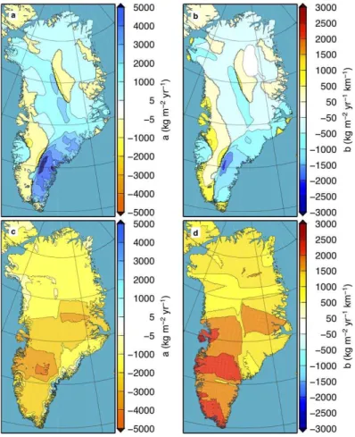
The climate data we use in this study is the 1958–2007 average SMB from the re-gional climate model RACMO2/GR (Fig. 1, Ettema et al., 2009). This rere-gional climate 5
model run is forced at its lateral boundaries by 6-hourly data from the global model of ECMWF, using ERA-40 reanalysis (Uppala et al., 2005) up to September 2002 and the operational analysis thereafter. The SMB field is calculated using a physical snow model, allowing an accurate description of refreezing of meltwater and the thermody-namic evolution of the upper snow/firn/ice layers, yielding a realistic reproduction of the 10
present-day SMB distribution with a high horizontal resolution (11×11 km). Note that
SMB is only calculated in RACMO2/GR for the area within the ice mask.
For each grid point, pairs ofHsand SMB are determined by selecting the data within a search radius of at least 150 km. A distinction is made between accumulation area and ablation area, and for each regime the search radius is extended in steps of 5 km 15
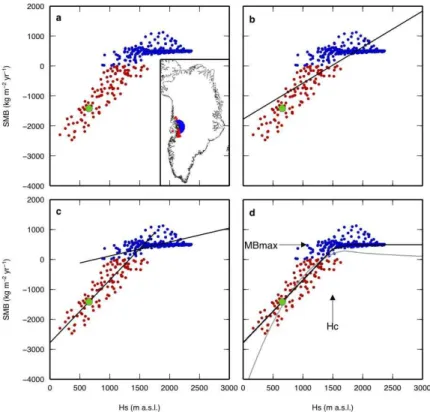
until a minimum amount ofHs-SMB pairs (n=100) is found. An example of a scatter plot ofHs and SMB data is shown in Fig. 2a, for a location in the ablation zone on the western margin of the GrIS. In this case, a search radius of 150 km is sufficient to find enough grid points in the accumulation area, but for the ablation area the search radius had to be extended to 225 km.
20
As shown in Fig. 2b, a simple linear regression through all (ablation and accumula-tion) points does not lead to a useful relation of SMB as a function ofHs. The SMB will then be largely overestimated at high values ofHs, especially forHs>2000 m. There-fore, we split the accumulation area and the ablation area, and construct separate linear relations for both regimes (Fig. 2c). Furthermore, as one of the boundary conditions 25
TCD
5, 2115–2157, 2011The mass balance gradient method
M. M. Helsen et al.
Title Page
Abstract Introduction
Conclusions References
Tables Figures
◭ ◮
◭ ◮
Back Close
Full Screen / Esc
Printer-friendly Version Interactive Discussion
Discussion
P
a
per
|
Dis
cussion
P
a
per
|
Discussion
P
a
per
|
Discussio
n
P
a
per
|
SMB(Hs,ref)=SMBref (1)
To this end, the linear regression line is forced through its reference value (green dot in Fig. 2) by adjusting the intercept of the lineafter the regression, without changing its slope. This method ensures a better representation of the SMB gradients then would be obtained with a regression that forces the line through the referenceHs-SMB point, 5
although the linear fits become slightly worse in a statistical sense by this treatment. Due to the scatter in theHs-SMB data, an ordinary linear regression does not always result in a good reconstruction of the transition from ablation area to accumulation area, nor does it lead to regression lines that are a good physical representation of the actualHs-SMB pattern. This is illustrated in Fig. 3, where the dashed lines are the linear 10
regression lines that follow from minimizing the vertical offsets between the data points and the regression line. The reconstructed equilibrium line altitude (ELA) is∼100 m
too high, and the transition height at which the ablation fit crosses the accumulation fit is also much too high. To improve this, instead of minimizing thevertical distances, we minimize theperpendicular distances between data points and regression line. This 15
method can only be used in scatter plots of data with equal units. To enable this, we first normalize the data on both axes, and then perform a linear regression by minimizing the perpendicular offsets (Fig. 3). Hereafter, regression equations are again rewritten to non-normalized form, such that SMB is predicted by:
SMB(Hs)= a
acc+baccHs if Hs> Hc
aabl+bablHs if Hs< Hc (2)
20
whereHcis the elevation of intersection between the two lines.
This method works well for a steady-state model run using the present-day climate forcing, when only small SMB adjustments are applied as a function of ice geometry changes. However, when temperature perturbation experiments are performed (see below), SMB patterns in the accumulation area are vulnerable to large changes. This 25
TCD
5, 2115–2157, 2011The mass balance gradient method
M. M. Helsen et al.
Title Page
Abstract Introduction
Conclusions References
Tables Figures
◭ ◮
◭ ◮
Back Close
Full Screen / Esc
Printer-friendly Version Interactive Discussion
Discussion
P
a
per
|
Dis
cussion
P
a
per
|
Discussion
P
a
per
|
Discussio
n
P
a
per
|
SMB, that becomes unrealistic with increasingHs(Figs. 2c and 3a). Negative values of
bacccan also lead to problematic SMB values, since these eventually lead to negative SMB values with increasingHs, which is not likely to occur in Greenland (Fig. 3c). To keep SMB within reasonable boundaries, several minimum and maximum constraints have been tested, and the following were considered most suitable and are introduced 5
for the accumulation regime:
SMBmax=max(SMBpos,SMBref) (3)
SMBmin= (
0.25×SMBpos if SMBref<0
0.25×SMBref if SMBref>0
(4)
The black lines in Figs. 2d, 3b and d are examples of the relations that are used to calculate SMB as a function of localHs. These regressions have been calculated for 10
each grid point within the domain, and results are shown in Fig. 4. The SMB gradients for the accumulation regime (baccin Eq. 2, Fig. 4b) are generally small (<0.001 yr−1), and mostly negative over the interior part of the ice sheet, apart from an area in the central north. bacc is positive along the western margin, implying decreasing run-off and/or an increase in accumulation with increasing elevation. The high accumulation 15
in the southeast is reflected by large positive values of the regression constantaacc in this area. Values ofbabl show a pattern from high values in the south(-west), to lower values in the north. The gradient of SMB in the western ablation zone is in the order of
∼2.5 m i.e. yr−1km−1.
This SBM parameterization allows us to calculate a continuous SMB field over the 20
entire domain, as a function of Hs, also for areas outside the present-day ice mask. This is required to provide the ice sheet model with a continuous SMB forcing, since ice-free areas along the periphery of the ice sheet quickly become ice covered if no negative SMB forcing is applied. Once grid points outside the present-day ice mask becomes ice covered, an SMB value is calculated based on data from currently ice-25
TCD
5, 2115–2157, 2011The mass balance gradient method
M. M. Helsen et al.
Title Page
Abstract Introduction
Conclusions References
Tables Figures
◭ ◮
◭ ◮
Back Close
Full Screen / Esc
Printer-friendly Version Interactive Discussion
Discussion
P
a
per
|
Dis
cussion
P
a
per
|
Discussion
P
a
per
|
Discussio
n
P
a
per
|
ice covered, a lower SMB value should be assigned than the value that follows from the parameterization, due to the influence of e.g. a much lower albedo of tundra compared to ice. To account for the influence of the tundra and hence correct for this possible flaw in SMB pattern, we subtract 1 m i.e. yr−1 from the calculated SMB when ice thickness is below 1 m. Different values for the treatment of SMB at the ice margin have been 5
tested, and these values prevented an unrealistic expansion of the simulated ice sheet over the entire mainland of Greenland under the present-day SMB forcing.
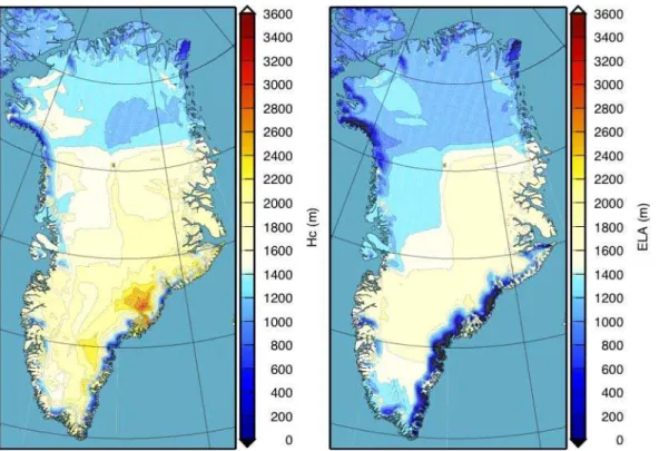
With this SMB parameterization it is possible to calculate the elevation of intersection (Hc) and the ELA for each individual grid point, assuming a fully ice-covered Greenland mainland for the SMB calculations (Fig. 5). As expected, a north-south gradient is 10
present in both patterns, of decreasing ELA with increasing latitude as this is present in the RACMO2/GR fields. The area with low ELA in the southeast is caused by the high accumulation in this area, prohibiting net ablation on the 11 km ice sheet mask (in reality the ablation zone is 1-several km wide). The east-west gradient over the north-ern part of the domain is due to the higher accumulation in the northwest compared to 15
the northeast.
2.2 Temperature adjustment by refreezing
Due to the temperature-dependence of the ice viscosity it is of great importance for the ice flow velocity to calculate the ice temperature by solving the thermodynamic equation. The temperature of the ice is determined by the ice advection, diffusion, 20
geothermal heat flux at the bottom, heat production due to ice deformation, friction of the ice at the bottom when its sliding over its bed, and the mean annual temperature at the surface (Ts). Here we use the RACMO2/GR 1958–2007 mean Ts for this lat-ter lat-term, and we correct for elevation changes using the atmospheric lapse rateγatm
(Table 1). Another process that will change the ice temperature is refreezing (R) of 25
percolating meltwater in firn layers. In the more classical treatment of SMB calculation in ice sheet models,R is often calculated on-line as a fraction of the annual ablation by making assumptions about the seasonal cycle of surface temperature and snowpack
TCD
5, 2115–2157, 2011The mass balance gradient method
M. M. Helsen et al.
Title Page
Abstract Introduction
Conclusions References
Tables Figures
◭ ◮
◭ ◮
Back Close
Full Screen / Esc
Printer-friendly Version Interactive Discussion
Discussion
P
a
per
|
Dis
cussion
P
a
per
|
Discussion
P
a
per
|
Discussio
n
P
a
per
|
characteristics. Hence the heat release that is associated byR can be taken into ac-count inTs.
In our modelling set up, the effect ofR on SMB is already taken into account in the regional climate model, so this effect is included in the net SMB values as we use here. However, we still need to take into account the thermodynamic effect ofR for the 5
calculation of ice temperatures. Thus, we can use the refreezing as a separate forcing field (Fig. 6), by applying a relation between R and the associated ice temperature warming as suggested by Reeh (1991):
∆Ts(R)=26.6R (5)
withR in m w.e. yr−1. 10
However, using a fixed field of R poses a comparable problem as for SMB, since
R will likely change with a changing ice geometry. Hence, we treat this problem in a similar way as we do for SMB, by calculating the gradients ofR as a function of Hs, using the same set of data points for each location as were used for the calculation of the SMB(Hs) relations. Figure 7 shows an example of such a relation for a location in 15
the northeast. As constraint for thisR(Hs) relation, we demand a positive gradient in the ablation regime, and a negative gradient in the accumulation regime.
2.3 SMB perturbations in climate change experiments
The SMB method as described above is well suited to be used in an asynchronously coupled climate-ice sheet model set-up: the SMB gradients method is used each time 20
step to account for changes in SMB field as a result of ice sheet elevation changes and extent. After a certain integration time of the ice sheet model, the ice sheet surface elevation and extent in the climate model should then be updated by the newHs field of the ice sheet model, such that the climate model can generate a new climatology over the ice sheet again, which can consequently be used as forcing for the ice sheet 25
TCD
5, 2115–2157, 2011The mass balance gradient method
M. M. Helsen et al.
Title Page
Abstract Introduction
Conclusions References
Tables Figures
◭ ◮
◭ ◮
Back Close
Full Screen / Esc
Printer-friendly Version Interactive Discussion
Discussion
P
a
per
|
Dis
cussion
P
a
per
|
Discussion
P
a
per
|
Discussio
n
P
a
per
|
However, ice sheet model experiments are often used to simulate the effect of climate perturbations, or reconstruct ice sheet behavior over glacial-interglacial time scale. Therefore, we also intend to test whether the SMB gradients as calculated here can be used to translate a climatic surface temperature perturbation that is applied uniformly over the ice sheet into a spatially differentiated change in SMB. To this end, we extend 5
our method by introducing an extra term in Eq. (2) that accounts for a SMB change as a function of a climate perturbation. Instead of using the actual ice sheet elevation (Hs) in Eq. (2), we use a climatic elevation (H∆T) that is adjusted as a function of a surface temperature perturbation (∆Tclimate):
H∆T=Hs+∆Tclimate
γatm (6)
10
Hence, for example a climate perturbation of+1◦C and usingγ
atm=−7.4 K km−1will
lead to a decrease ofH∆T of 135 m. With a typical SMB gradient of 2 m i.e. yr−1km−1 in the ablation regime this leads to a drop in SMB of 0.27 m i.e. yr−1. Note that since SMB gradients differ spatially, an identical temperature change will lead to regionally different SMB adjustments.
15
2.4 Ice sheet model
To test this new method of SMB forcing on an ice sheet model for the GrIS, we use the 3-D thermomechanical model ANICE (e.g. Van de Wal, 1999a,b; Bintanja et al., 2005; Bintanja and Van de Wal, 2008; Van den Berg et al., 2008; Graversen et al., 2010) based on the shallow ice approximation (SIA, Hutter, 1983), and including ther-20
modynamics to explicitly account for the temperature-dependent stiffness of the ice. Hence, ice temperature is calculated based on the 3-D advection, diffusion, friction, geothermal heat flux (G) at the bottom and annual surface temperature (Ts) adjusted for the effect of refreezing (Sect. 2.2). The vertical dimension is scaled with the local ice thickness, and consists of 15 layers with increasing resolution near the bed, to ac-25
TCD
5, 2115–2157, 2011The mass balance gradient method
M. M. Helsen et al.
Title Page
Abstract Introduction
Conclusions References
Tables Figures
◭ ◮
◭ ◮
Back Close
Full Screen / Esc
Printer-friendly Version Interactive Discussion
Discussion
P
a
per
|
Dis
cussion
P
a
per
|
Discussion
P
a
per
|
Discussio
n
P
a
per
|
basal temperatures reach the pressure melting point we allow the ice to slide over its bed, by using a Weertman-type sliding law (Weertman, 1964), corrected for the effect of subglacial water pressure (Bindschadler, 1983). Formation of ice shelves is not al-lowed; as soon as the ice thickness becomes small enough that it will go afloat and ice is in contact with the ocean, the ice breaks off. As such, calving by means of a flotation 5
criterion is included, but more detailed calving physics are not incorporated explicitly, since model resolution and dynamics are not suited for a more realistic treatment of calving of outlet glaciers. The response of a changing ice load on bedrock elevation is taken into account using an Elastic Litosphere-Relaxing Astenosphere (ELRA) model (Le Meur and Huybrechts, 1996). As such, the ice sheet model is a traditional SIA 10
model including thermodynamics and bedrock adjustment. Table 1 summarizes the values for different parameters used in all components of the ice sheet model.
2.5 Model set up
The different model components (ice flow, thermodynamics, SMB, and bedrock re-sponse) are coupled and applied on a rectangular domain of 141×77 grid points with
15
a grid spacing of 20 km. Bedrock elevation (Hb) and ice thickness (Hi) fields are from Bamber et al. (2001b), and these fields are interpolated to our ice model grid using the mapping package OBLIMAP (Reerink et al., 2010), using an oblique stereographic projection centered at 72◦N, 40◦W, with projection angleα
=7.5◦. The same mapping configuration is used to interpolate fields of SMB,Ts and R from the regional climate 20
model RACMO2/GR, and the spatially differentiated functions for SMB(Hs) andR(Hs) are interpolated likewise.
A difference exists between the areal extent of the GrIS ice thickness data as pre-sented in Bamber et al. (2001b) and the arial extent of the ice mask in Bamber et al. (2001a), the latter also containing the spatial distribution of numerous small ice caps 25
TCD
5, 2115–2157, 2011The mass balance gradient method
M. M. Helsen et al.
Title Page
Abstract Introduction
Conclusions References
Tables Figures
◭ ◮
◭ ◮
Back Close
Full Screen / Esc
Printer-friendly Version Interactive Discussion
Discussion
P
a
per
|
Dis
cussion
P
a
per
|
Discussion
P
a
per
|
Discussio
n
P
a
per
|
ice thickness. Since SMB from Ettema et al. (2009) is available for the ice mask from Bamber et al. (2001a), we apply a correction to our initial ice thickness field from Bam-ber et al. (2001b) by assigning a 10 m thick ice layer to all grid points within the ice mask but where ice thickness data is missing, and let the model freely evolve from there.
5
Initialization of the 3-D temperature field is done by using the Robin solution based onTs,Gand SMB in the accumulation zone. Ice temperatures in the ablation zone are initialized as a linear profile betweenTs and the pressure melting point.
3 Results
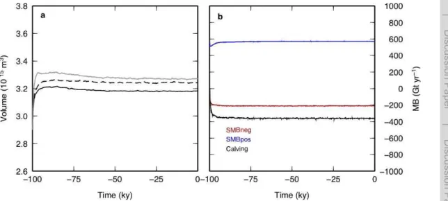
3.1 Reference experiment 10
To test the performance of our parameterizations for SMB andR, we start with a steady-state run of 100 ky using constant present-day forcing, so no additional climate change forcing. Figure 8a shows the evolution of ice volume during this simulation. The ice vol-ume initially quickly increases, from the present-day observed value of 2.90×10¹⁵m3
to 3.20×10¹⁵m3within 10 ky. After∼30 ky the ice volume has leveled offto its
steady-15
state value of 3.18×10¹⁵m3, 10 % above the observed GrIS volume. It should be
noted that only ice on the Greenland mainland has been taken into account; the ice on Ellesmere Island has been removed from this summation.
The dashed black line in Fig. 8a illustrates the results obtained when the effect of refreezing is neglected. This results in a slightly larger ice sheet, due to slightly lower 20
ice temperatures, that influence both deformation rate and the occurrence of sliding. Hence, ice velocity is slightly lower in the non-refreezing experiment, resulting in a slightly higher steady-state ice volume.
Figure 9a shows ice sheet extent andHs of the steady-state ice sheet after 100 ky, and Fig. 9b illustrates the difference inHs compared to the present-day state. The ice 25
sheet has advanced along large parts of its margin, especially in the southwest, along its eastern margin and in the north.
TCD
5, 2115–2157, 2011The mass balance gradient method
M. M. Helsen et al.
Title Page
Abstract Introduction
Conclusions References
Tables Figures
◭ ◮
◭ ◮
Back Close
Full Screen / Esc
Printer-friendly Version Interactive Discussion
Discussion
P
a
per
|
Dis
cussion
P
a
per
|
Discussion
P
a
per
|
Discussio
n
P
a
per
|
Figure 8b shows the different mass balance terms as a function of time. The term SMBpos and SMBnegcontain the integrated values of SMB over the accumulation area and ablation area, respectively. Hence these terms cannot be compared with the ice-sheet integrated accumulation and run-off terms. The steady-state integrated SMB equals 362 Gt yr−1, and is in balance with the calving flux. This is 23 % lower than 5
the total ice sheet SMB value of 469 Gt yr−1 from RACMO2/GR (Ettema et al., 2009), and this large difference can be explained by an expansion of the total ablation area, reducing the integrated ice sheet SMB.
The expansion of the ice sheet in the south inevitably occurs due to the high accu-mulation in combination with the (initial) absence of a significant ablation zone along 10
large stretches of the margin, for example in the southeast (Fig. 1). In reality, most of the ice in this area is lost by calving of fast-flowing outlet glaciers, that export ice to the ocean where it is released by calving. These glaciers flow through deep, narrow fjords that characterize the topography in this area. This process is not well-described in our simulations, due to two reasons: (1) these narrow fjords are not resolved in the 15
20 km grid, effectively leading to a seaward displacement of the model coastline; and (2) our SIA-type model does neither accurately describe fast flowing glaciers, nor the calving process. This leads to an ice margin advance towards the coast in our simu-lation, increasing the calving flux, and also allows the formation of an ablation zone in areas that were previously ice-free (Fig. 10). It should be noted here that increasing 20
the resolution to 10 km does not improve the results; outlet glaciers in these fjords have typical widths of less than 5 km.
The pattern of a margin closer to the coast in combination with a slightly thinner interior ice sheet is a typical phenomena that has been found in many ice sheet mod-elling studies (e.g. Greve, 2005; Graversen et al., 2010; Robinson et al., 2010). The 25
TCD
5, 2115–2157, 2011The mass balance gradient method
M. M. Helsen et al.
Title Page
Abstract Introduction
Conclusions References
Tables Figures
◭ ◮
◭ ◮
Back Close
Full Screen / Esc
Printer-friendly Version Interactive Discussion
Discussion
P
a
per
|
Dis
cussion
P
a
per
|
Discussion
P
a
per
|
Discussio
n
P
a
per
|
The resulting mass balance pattern (Fig. 10) is in good agreement with the origi-nal fields (Fig. 1), which is not surprising as it is based on the RACMO2/GR run for present-day SMB, though elevations are slightly different. Differences occur along the eastern margin where lower SMB values are reconstructed due to higher elevations in combination with negative SMB gradients in the accumulation area. Reconstructed 5
SMB is higher than the original values in the western ablation area, where ice sheet elevations are again higher, but here the SMB gradients are positive.
3.2 Temperature perturbations
As a first indication of the performance of our method, the ice-sheet integrated SMB is assessed as a function of∆Tclimate (Table 2). Obviously, decreasing SMB values are 10
obtained with increasing temperature perturbations. Net SMB becomes negative only at climate perturbations of 4 K and higher, but also for smaller climate perturbations the ice sheet will shrink, as is described below.
A set of temperature-perturbation experiments was carried out, for which the results are shown in Fig. 11. The steady-state ice sheet is perturbed with a certain∆Tclimate, for 15
another 100 ky, to reach a new equilibrium state. The perturbation has a direct SMB ef-fect and an indirect (thermo-)dynamic effect on ice volume. The effect of a temperature perturbation on SMB is controlled by Eqs. (2) and (6), and the dominant mechanism is that (obviously) a cooler climate will results in a more extensive accumulation area and smaller ablation rates in the ablation area. However, accumulation areas with negative 20
SMB gradients (bacc) will effectively receive less accumulation, which can regionally result in a net decrease of the integrated SMB.
Both ice sheet extent (Fig. 11a) and ice volume (Fig. 11b) show a clear nonlinear relation with the applied temperature perturbation, with much stronger effects with pos-itive values of∆Tclimate. The ice sheet extent hardly increases with lower temperatures, 25
since it almost entirely fills the island of Greenland. Increased ice volume is thus mainly due to thickening of the ice sheet. A slight decrease in ice volume can be identified in the experiments with a temperature perturbations in the range of∆Tclimate=−5−0 K.
TCD
5, 2115–2157, 2011The mass balance gradient method
M. M. Helsen et al.
Title Page
Abstract Introduction
Conclusions References
Tables Figures
◭ ◮
◭ ◮
Back Close
Full Screen / Esc
Printer-friendly Version Interactive Discussion
Discussion
P
a
per
|
Dis
cussion
P
a
per
|
Discussion
P
a
per
|
Discussio
n
P
a
per
|
This is due to the decreasing SMB values in the accumulation area, which outweighs the effect of enlargement of the accumulation area.
A huge difference in ice sheet size occurs between the +1 and +2 K experiments. Care must be taken with the quantitative robustness of this result, since it is highly dependent on the the value of γatm in Eq. (6). However, in a qualitative sense this 5
nonlinear behavior of the GrIS is likely realistic, i.e. that a threshold value exists for the SMB perturbation, above which the GrIS will eventually retreat to only a fraction of its current size. This is in agreement with Van de Wal (e.g. 1999a), who did a set of similar experiments using the same ice dynamical model, but using a different approach to estimate the SMB forcing.
10
This set of temperature perturbation experiments has also been carried out for a model set-up neglecting the effect of refreezing (not shown). Although the temperature adjustment due to refreezing can be substantial (Fig. 6), the influence of this effect on the final results in terms of ice volume are mostly only minor (see e.g. Fig. 8). However, for certain values of∆Tclimate steady-state ice volume is significantly higher when the 15
effect of refreezing on ice temperature is not taken into account. 3.3 Simulating a full glacial cycle
In analogy with e.g. Letr ´eguilly et al. (1991); Van de Wal (1999a); Greve (2005), we also performed an experiment that aims to describe the GrIS evolution through a full glacial cycle. The climate record used as a proxy for∆Tclimate is based on the GRIP 20
δ18O record (Johnsen et al., 2001), and converted into a surface temperature deviation following Johnsen et al. (1995). Prior to 105 ky, the GRIP record is not a valid climate proxy due to ice-flow irregularities (North Greenland Ice Core Project members, 2004), so for this period we use the VostokδDrecord and blend the two records in a similar may as described in Greve (2005). This temperature forcing is applied uniformly over 25
TCD
5, 2115–2157, 2011The mass balance gradient method
M. M. Helsen et al.
Title Page
Abstract Introduction
Conclusions References
Tables Figures
◭ ◮
◭ ◮
Back Close
Full Screen / Esc
Printer-friendly Version Interactive Discussion
Discussion
P
a
per
|
Dis
cussion
P
a
per
|
Discussion
P
a
per
|
Discussio
n
P
a
per
|
climate optimum, using the present-day ice thickness as initial conditions, just as in the reference experiment (Sect. 3.1).
Figure 12 shows ice sheet volume as a response on the climate forcing through the glacial cycle. We do not show minimum Eemian ice volume, since no value should be attributed to this value considering the dependence on initial conditions. The simulated 5
increase in ice volume through the glacial culminates in a peak LGM ice volume of 3.56×10¹⁵m3, which is in the lower range of most earlier reconstructions obtained by
ice flow models (e.g. Van de Wal, 1999a; Huybrechts, 2002; Robinson et al., 2010) and paleoclimatic evidence (Fleming and Lambeck, 2004), but slightly higher than the reconstruction by Greve (2005). This low LGM ice volume is a least partly caused by 10
the lack of ice shelf dynamics in our model, prohibiting merging of the GrIS and the Ellesmere Island section of the Laurentide Ice Sheet during the last glacial, which did occur in reality (England, 1999; Alley et al., 2010).
The simulated deglaciation results in a present-day ice sheet volume close to the steady-state volume. Also ice sheet elevation and extent resulting from this climate 15
experiment (Fig. 13) is in reasonable agreement with the observed present-day ele-vation. Comparison with the steady-state experiment (Fig. 9) shows that a realistic climatic forcing results in an improved ice sheet elevation in the interior. The location of the summit is slightly shifted towards the north, but inland elevations are not under-estimated anymore (like in the steady-state experiment, Fig. 9) due to the presence of 20
colder ice and its effect on ice stiffness. Two marginal areas in the southwest and north-west stand out (arrows in Fig. 13) because they are thinner than presently observed, and also contain wide ablation areas with SMB values lower than present (Fig. 14). These areas presently also contain wide ablation areas, which highlights the sensitivity of these areas to surface melting.
25
TCD
5, 2115–2157, 2011The mass balance gradient method
M. M. Helsen et al.
Title Page
Abstract Introduction
Conclusions References
Tables Figures
◭ ◮
◭ ◮
Back Close
Full Screen / Esc
Printer-friendly Version Interactive Discussion
Discussion
P
a
per
|
Dis
cussion
P
a
per
|
Discussion
P
a
per
|
Discussio
n
P
a
per
|
4 Discussion
The SMB method as presented here is in principle designed as a tool to improve asyn-chronous coupling between climate models and ice sheet models, but as shown here it can also be used as a stand-alone SMB forcing module, without multiple couplings to a climate model. To assess the performance of the method, the spatial SMB gradi-5
ents as used here should ideally be compared with temporal SMB gradients that can be reconstructed from multiple climate model runs using different fields of ice sheet elevation and extent. This is beyond the scope of this study, but will be assessed in future work.
To illustrate the influence of the SMB forcing on the outcome of ice sheet reconstruc-10
tions, we can however compare this method with the performance of a PDD model. Choices of parameterizations in the PDD model are made such that the resulting ice sheet integrated value of SMBPDDis in good agreement with the present-day observed value reported by Ettema et al. (2009) (Appendix A). The grey lines in Figs. 2d, 3b and 3d show SMB functions resulting from this PDD method. Values of SMBPDD are 15
calculated using different values of mean annual temperature as input for the PDD model, but to facilitate comparison with the SMB gradient method, the results are plot-ted as a function of elevation, using γatm to translate ∆Ts to Hs. Generally, the PDD method results in steeper SMB gradients in the ablation regimes, which results in larger ablation rates with decreasing elevation. The example of Fig. 2d also shows that the 20
PDD method does not reproduce the higher positive SMB values as currently found higher up in the accumulation regime, due to a too strong decrease of the accumula-tion with increasing elevaaccumula-tion.
Figure 15 shows a comparison of the SMB pattern calculated by the PDD model (Appendix A) as obtained for the present-day ice sheet with the SMB field from Ettema 25
TCD
5, 2115–2157, 2011The mass balance gradient method
M. M. Helsen et al.
Title Page
Abstract Introduction
Conclusions References
Tables Figures
◭ ◮
◭ ◮
Back Close
Full Screen / Esc
Printer-friendly Version Interactive Discussion
Discussion
P
a
per
|
Dis
cussion
P
a
per
|
Discussion
P
a
per
|
Discussio
n
P
a
per
|
SMB field from Ettema et al. (2009) (Fig. 15b) suggest that the PDD method results in steeper SMB gradients. This has consequences for any applied climate perturba-tion, as can also be concluded from Table 2, that shows that differences in ice-sheet integrated SMB values increase with increasing magnitude of the climate perturbation. When the steady-state climate perturbation experiments are repeated using the PDD 5
method (crosses in Fig. 11), several differences can be identified. Maximum ice sheet volumes are found for smaller negative values of ∆Tclimate, while the SMB gradient method results in a slight decrease of ice volume for these∆Tclimateexperiments due to decreasing SMB in the accumulation area. A decrease of ice volume due to decreasing precipitation also occurs in the PDD method, but only becomes the dominant effect at 10
large negative temperature perturbations. Results for the positive temperature pertur-bations are particularly different for the+2 K scenario, where the PDD forcing allows for a steady-state GrIS volume of intermediate size (∼1.7×10¹⁵m3), whereas using the
SMB gradient forcing results in a nearly total GrIS retreat. Not surprisingly, applying the PDD forcing for the glacial cycle experiment also results in a different reconstruction 15
(grey line in Fig. 13).
Comparing the results obtained by the different SMB methods cannot distinguish which of the methods gives best results, but it merely illustrates the large importance of the SMB forcing on the outcome of GrIS model simulations. Therefore, the best approach for correct estimation of changes in the SMB as a result of changes in ice 20
sheet elevation and extent is to use frequent coupling between the ice sheet model and a (regional) climate model. The SMB gradient method is designed to be used in between these couplings, with the assumption that regional SMB variability is a better predictor of the adjustment in SMB due to ice sheet geometry changes, rather then a correlation between temperature and SMB (as is done in the PDD approach).
25
Simulated ice sheet volume and extent resulting from this study are within the range of known reconstructions with similar ice sheet models. A note on the excess of ice along the (predominantly eastern) margin is warranted here. It seems a persisting feature in ice sheet model reconstructions (e.g. Greve, 2005; Graversen et al., 2010;
TCD
5, 2115–2157, 2011The mass balance gradient method
M. M. Helsen et al.
Title Page
Abstract Introduction
Conclusions References
Tables Figures
◭ ◮
◭ ◮
Back Close
Full Screen / Esc
Printer-friendly Version Interactive Discussion
Discussion
P
a
per
|
Dis
cussion
P
a
per
|
Discussion
P
a
per
|
Discussio
n
P
a
per
|
Robinson et al., 2010), which has become more prominent since improved bedrock topography (Bamber et al., 2001b) and improved climate fields (e.g. Ettema et al., 2009) have become available. The east coast of Greenland consists of rugged terrain, and receives relatively high amounts of precipitation. The narrow ablation area is too small to be properly resolved and to keep the ice margin in place, inducing glacial advance 5
in the model in the direction of the coast. Once glaciated, this area remains covered with ice. Improvements can be expected from model grids that have<1 km resolution, resolving the narrow fjords, in combination with higher order ice sheet models, with better description of fast outlet glacier dynamics, and possibly resolving steeper SMB gradients near the ice margin.
10
5 Conclusions
We have presented a novel approach to use SMB fields from regional climate models as a forcing for ice sheet models, accounting for the height-mass balance feedback within an ice sheet model simulation. Using the spatial relation between elevation and SMB, a distributed field of SMB gradients is calculated, both for the accumulation 15
regime and the ablation regime, such that SMB values can be retrieved as a function of elevation for each regime, and over the entire domain. It enables a dynamic SMB forcing of ice sheet models, also for initially non-glaciated areas in the peripheral areas of an ice sheet. The method is applied to the Greenland Ice Sheet (GrIS). Model ex-periments using both steady-state forcing and more realistic glacial-interglacial forcing 20
TCD
5, 2115–2157, 2011The mass balance gradient method
M. M. Helsen et al.
Title Page
Abstract Introduction
Conclusions References
Tables Figures
◭ ◮
◭ ◮
Back Close
Full Screen / Esc
Printer-friendly Version Interactive Discussion
Discussion
P
a
per
|
Dis
cussion
P
a
per
|
Discussion
P
a
per
|
Discussio
n
P
a
per
|
Appendix A
PDD method
To facilitate comparison of our results obtained with the SMB gradient method with results from a PDD model, we also performed experiments driven with SMB fields 5
from a PDD-model, which is briefly described here. This method relies on a statistical relationship between positive air temperatures and melt rates of snow and ice (e.g. Braithwaite and Olesen, 1989; Reeh, 1991). When using a PDD model, a suite of choices exist in parameterizations that can be used to drive the model. Here we made these choices such that the PDD model produced an ice sheet integrated SMB value 10
in close agreement with the SMB from RACMO2/GR on the initial ice sheet mask. We allow the degree-day factors to be different for snow and ice, and also for warm and cold climate conditions, using the expressions from Tarasov and Peltier (2002). Following Greve (2005), we assume warm climate conditions south of 72◦N. PDDs are calculated on a monthly basis, based on a sinusoidal temperature cycle over a 15
year, in combination with a statistical air temperature fluctuation (σ=5.2, Tarasov and Peltier, 2002) to account for random temperature fluctuations and the daily cycle. The semi-analytical solution by Calov and Greve (2005) is used to calculated the positive degree-day integral.
To avoid any discrepancy in forcing, we also use RACMO2/GR 1958–2007 mean 20
Ts to drive the PDD model. Superimposed on this the seasonal temperature cycle is estimated using the parameterization from Huybrechts and de Wolde (1999). Recently Fausto et al. (2009) suggested improved parameterizations of surface temperature over Greenland, but using these resulted in large deviations of the resulting SMB values with respect to the RACMO2/GR fields.
25
For accumulation we use 1958–2007 mean precipitation fields (Ettema et al., 2009), from which we calculate a rain fraction based on the time near-surface temperature is above+2◦C (Huybrechts and de Wolde, 1999). To account for precipitation changes
TCD
5, 2115–2157, 2011The mass balance gradient method
M. M. Helsen et al.
Title Page
Abstract Introduction
Conclusions References
Tables Figures
◭ ◮
◭ ◮
Back Close
Full Screen / Esc
Printer-friendly Version Interactive Discussion
Discussion
P
a
per
|
Dis
cussion
P
a
per
|
Discussion
P
a
per
|
Discussio
n
P
a
per
|
in different climate settings, the present-day precipitation climatology is adjusted as a function of∆Ts(Huybrechts and de Wolde, 1999).
The liquid water that is formed (rain and meltwater) is allowed to refreeze, to form superimposed ice, with a maximum based on the cold content of the surface snow layer (Huybrechts and de Wolde, 1999).
5
Acknowledgements. We would like to thank Thomas Reerink for his role in the development of the ANICE ice sheet model.
References
Alley, R. B., Andrews, J. T., Brigham-Grette, J., Clarke, G. K. C., Cuffey, K. M., Fitzpatrick, J. J., Funder, S., Marshall, S. J., Miller, G. H., Mitrovica, J. X., Muhs, D. R., Otto-Bliesner, B. L.,
10
Polyak, L., and White, J. W. C.: History of the Greenland Ice Sheet: Paleoclimatic insights, Quaternary Sci. Rev., 29, 1674–1790, 2010. 2131
Bales, R. C., Guo, Q., Shen, D., McConnell, J. R., Du, G., Burkhart, J. F., Spikes, V. B., Hanna, E., and Cappelen, J.: Annual accumulation for Greenland updated using ice core data devel-oped during 2000–2006 and analysis of daily coastal meteorological data, J. Geophys. Res.,
15
114, D06116, doi:10.1029/2008JD011208, 2009. 2117
Bamber, J. L., Ekholm, S., and Krabill, W.: A new, high-resolution digital elevation model of Greenland fully validated with airborne laser altimeter data, J. Geophys. Res., 106, 6733– 6745, 2001a. 2126, 2127
Bamber, J. L., Layberry, R. L., and Gogineni, S. P.: A new ice thickness and bed data set for
20
the Greenland ice sheet 1. Measurement, data reduction, and errors, J. Geophys. Res., 106, 33773–33780, 2001b. 2126, 2127, 2134
Bindschadler, R.: The importance of pressurized subglacial water in separation and sliding and the glacial bed, J. Glaciol., 29, 3–19, 1983. 2126
Bintanja, R. and Van de Wal, R. S. W.: North American ice-sheet dynamics and the onset of
25
100,000-year glacial cycles, Nature, 454, 869–872, 2008. 2125, 2130
TCD
5, 2115–2157, 2011The mass balance gradient method
M. M. Helsen et al.
Title Page
Abstract Introduction
Conclusions References
Tables Figures
◭ ◮
◭ ◮
Back Close
Full Screen / Esc
Printer-friendly Version Interactive Discussion
Discussion
P
a
per
|
Dis
cussion
P
a
per
|
Discussion
P
a
per
|
Discussio
n
P
a
per
|
Bougamont, M., Bamber, J. L., Ridley, J. K., Gladstone, R. M., Greuell, W., Hanna, E., Payne, A. J., and Rutt, I.: Impact of model physics on estimating the surface mass balance of the Greenland ice sheet, Geophys. Res. Lett., 34, L17501, doi:10.1029/2007GL030700, 2007. 2118
Box, J. E., Bromwich, D. H., Veenhuis, B. A., Bai, L.-E., Stroeve, J. C., Rogers, J. C., Steffen, K.,
5
Haran, T., and Wang, S.-H.: Greenland Ice Sheet Surface Mass Balance Variability (1988– 2004) from Calibrated Polar MM5 Output, J. Climate, 19, 2783–2800, 2006. 2117
Braithwaite, R. J. and Olesen, O. B.: Glacier fluctuations and climatic change, chap. Calcula-tion of glacier ablaCalcula-tion from air temperature, West Greenland, Kluwer Academic Publishers, Dordrecht, 219–233, 1989. 2118, 2135
10
Calov, R. and Greve, R.: A semi-analytical solution for the positive degree-day model with stochastic temperature variations, J. Glaciol., 51, 173–175, 2005. 2135
Charbit, S., Ritz, C., and Ramstein, G.: Simulations of Northern Hemisphere ice-sheet retreat: sensitivity to physical mechanisms involved during the Last Deglaciation, Quaternary Sci. Rev., 21, 243–265, 2002. 2118
15
England, J.: Coalescent Greenland and Innuitian ice during the Last Glacial Maximum – rivising the Quaternary of the Canadian High Arctic, Quaternary Sci. Rev., 18, 421–456, 1999. 2131 Ettema, J., Van den Broeke, M. R., van Meijgaard, E., van de Berg, W. J., Bamber, J. L., Box, J. E., and Bales, R. C.: Higher surface mass balance of the Greenland ice sheet revealed by high-resolution climate modeling, Geophys. Res. Lett., 36, L12501,
20
doi:10.1029/2009GL038110, 2009. 2117, 2118, 2120, 2127, 2128, 2132, 2133, 2134, 2135, 2143, 2148, 2152, 2156, 2157
Fausto, R., Ahlstrøm, A. P., Van As, D., Bøggild, C. E., and Johnsen, S. J.: A new present-day temperature parameterization for Greenland, J. Glaciol., 55, 95–105, 2009. 2135
Fettweis, X., Hanna, E., Gall ´ee, H., Huybrechts, P., and Erpicum, M.: Estimation of the
Green-25
land ice sheet surface mass balance for the 20th and 21st centuries, The Cryosphere, 2, 117–129, doi:10.5194/tc-2-117-2008, 2008. 2117
Fleming, K. and Lambeck, K.: Constraints on the Greenland Ice Sheet since the Last Glacial Maximum from sea-level observations and glacial-rebound models, Quaternary Sci. Rev., 23, 1053–1077, 2004. 2131
30
Graversen, R. G., Drijfhout, S., Hazeleger, W., Van de Wal, R., Bintanja, R., and Helsen, M.: Greenland’s contribution to global sea-level rise by the end of the 21st century, Clim. Dynam., 1–16, 2010. 2116, 2117, 2125, 2128, 2133
TCD
5, 2115–2157, 2011The mass balance gradient method
M. M. Helsen et al.
Title Page
Abstract Introduction
Conclusions References
Tables Figures
◭ ◮
◭ ◮
Back Close
Full Screen / Esc
Printer-friendly Version Interactive Discussion
Discussion
P
a
per
|
Dis
cussion
P
a
per
|
Discussion
P
a
per
|
Discussio
n
P
a
per
|
Greve, R.: Relation of measured basal temperatures and the spatial distribution of the geothermal heat flux for the Greenland ice sheet, Ann. Glaciol., 42, 424–432, 2005. 2128, 2130, 2131, 2133, 2135
Hutter, K.: Theoretical glaciology: material science of ice and the mechanics of glaciers and ice sheets, Reidel Publ. Co., Dordrecht, 1983. 2125
5
Huybrechts, P.: The present evolution of the Greenland ice sheet:an assessment by modelling, Global Planet. Change, 9, 39–51, 1994. 2116, 2117
Huybrechts, P.: Sea-level changes at the LGM from ice-dynamic reconstructions of the Green-land and Antarctic ice sheets during the glacial cycles, Quaternary Sci. Rev., 21, 203–231, 2002. 2131
10
Huybrechts, P. and de Wolde, J.: The dynamic responce of the Greenland and Antarctic ice sheets to multiple century climate warming, J. Climate, 12, 2169–2188, 1999. 2135, 2136 Huybrechts, P., Letr ´eguilly, A., and Reeh, N.: The Greenland ice sheet and greenhouse
warm-ing, Palaeogeogr. Palaeocl., 89, 399–412, 1991. 2116
Huybrechts, P., Gregory, J., Janssens, I., and Wild, M.: Modelling Antarctic and Greenland
15
volume changes during the 20th and 21st centuries forced by GCM time slice integrations, Global Planet. Change, 42, 83–105, 2004. 2117
Johnsen, S. J., Dahl-Jensen, D., Dansgaard, W., and Gundestrup, N.: Greenland palaeotem-peratures derived from GRIP bore hole temperature and ice core isotope profiles, Tellus, 47B, 624–629, 1995. 2130
20
Johnsen, S. J., Dahl-Jensen, D., Gundestrup, N., Steffensen, J. P., Clausen, H. B., Miller, H., Masson-Delmotte, V., Sveinbj ¨orndottir, A. E., and White, J.: Oxygen isotope and palaeotem-perature records from six Greenland ice-core stations: Camp Century, Dye-3, GRIP, GISP2, Renland and NorthGRIP, J. Quaternary Sci., 16, 299–307, 2001. 2130
Kiehl, J. T. and Gent, P. R.: The Community Climate System Model, Version 2, J. Climate, 17,
25
3666–3682, 2004. 2117
Le Meur, E. and Huybrechts, P.: A comparison of different ways of dealing with isostasy: ex-amples from modelling the Antarctic ice sheet during the last glacial cycle, Ann. Glaciol., 23, 309–317, 1996. 2126
Letr ´eguilly, A., Huybrechts, P., and Reeh, N.: Steady-state characteristics of the Greenland ice
30
sheet under different climate states, J. Glaciol., 37, 149–157, 1991. 2116, 2117, 2130 Lhomme, N., Clarke, G. K. C., and Marshall, S. J.: Tracer transport in the Greenland ice sheet:
TCD
5, 2115–2157, 2011The mass balance gradient method
M. M. Helsen et al.
Title Page
Abstract Introduction
Conclusions References
Tables Figures
◭ ◮
◭ ◮
Back Close
Full Screen / Esc
Printer-friendly Version Interactive Discussion
Discussion
P
a
per
|
Dis
cussion
P
a
per
|
Discussion
P
a
per
|
Discussio
n
P
a
per
|
Marshall, S. J. and Cuffey, K. M.: Peregrinations of the Greenland Ice Sheet divide in the last glacial cycle: implications for central Greenland ice cores, Earth Planet. Sc. Lett., 179, 73– 90, 2000. 2116
North Greenland Ice Core Project members: High-resolution record of Northern Hemisphere climate extending into the last interglacial period, Nature, 431, 147–151, 2004. 2130
5
Ohmura, A. and Reeh, N.: New precipitation and accumulation maps for Greenland, J. Glaciol., 37, 140–148, 1991. 2117
Otto-Bliesner, B., Marshall, S. J., Overpeck, J. T., Miller, G. H., Hu, A., and Members, C. L. I. P.: Simulating Arctic climate warmth and icefield retreat in the last interglaciation, Science, 311, 1751–1753, 2006. 2116, 2117
10
Reeh, N.: Parameterization of melt rate and surface temperature on the Greenland ice sheet, Polarforschung, 59, 113–128, 1991. 2118, 2124, 2135, 2148
Reerink, T. J., Kliphuis, M. A., and van de Wal, R. S. W.: Mapping technique of climate fields between GCM’s and ice models, Geosci. Model Dev., 3, 13–41, doi:10.5194/gmd-3-13-2010, 2010. 2126
15
Ritz, C., Fabre, A., and Letr ´eguilly, A.: Sensitivity of a Greenland ice sheet model to ice flow and ablation parameters: consequences for the evolution through the last climatic cycle, Clim. Dynamics, 13, 11–24, 1997. 2117
Robinson, A., Calov, R., and Ganopolski, A.: An efficient regional energy-moisture bal-ance model for simulation of the Greenland Ice Sheet response to climate change, The
20
Cryosphere, 4, 129–144, doi:10.5194/tc-4-129-2010, 2010. 2117, 2118, 2128, 2131, 2134 Robinson, A., Calov, R., and Ganopolski, A.: Greenland ice sheet model parameters
con-strained using simulations of the Eemian Interglacial, Clim. Past, 7, 381–396, doi:10.5194/cp-7-381-2011, 2011. 2116, 2117
Tarasov, L. and Peltier, W. R.: Greenland glacial history and local geodynamic consequences,
25
Geophys. J. Int., 150, 198–229, 2002. 2135
Uppala, S. M., K ˚Allberg, P. W., Simmons, A. J., Andrae, U., Bechtold, V. D. C., Fiorino, M., Gibson, J. K., Haseler, J., Hernandez, A., Kelly, G. A., Li, X., Onogi, K., Saarinen, S., Sokka, N., Allan, R. P., Andersson, E., Arpe, K., Balmaseda, M. A., Beljaars, A. C. M., Berg, L. V. D., Bidlot, J., Bormann, N., Caires, S., Chevallier, F., Dethof, A., Dragosavac, M., Fisher,
30
M., Fuentes, M., Hagemann, S., H ´olm, E., Hoskins, B. J., Isaksen, L., Janssen, P. A. E. M., Jenne, R., Mcnally, A. P., Mahfouf, J.-F., Morcrette, J.-J., Rayner, N. A., Saunders, R. W., Simon, P., Sterl, A., Trenberth, K. E., Untch, A., Vasiljevic, D., Viterbo, P., and Woollen, J.:
TCD
5, 2115–2157, 2011The mass balance gradient method
M. M. Helsen et al.
Title Page
Abstract Introduction
Conclusions References
Tables Figures
◭ ◮
◭ ◮
Back Close
Full Screen / Esc
Printer-friendly Version Interactive Discussion
Discussion
P
a
per
|
Dis
cussion
P
a
per
|
Discussion
P
a
per
|
Discussio
n
P
a
per
|
The ERA-40 re-analysis, Q. J. Roy. Meteorol. Soc., 131, 2961–3012, doi:10.1256/qj.04.176, 2005. 2117, 2120
Van de Wal, R. S. W.: Mass-balance modelling of the Greenland ice sheet: a comparison of an energy-balance and a degree-day model, Ann. Glaciol., 23, 36–45, 1996. 2118
Van de Wal, R. S. W.: The importance of thermodynamics for modeling the volume of the
5
Greenland ice sheet, J. Geophys. Res., 104, 3889–3898, 1999a. 2125, 2130, 2131
Van de Wal, R. S. W.: Processes of buildup and retreat of the Greenland ice sheet, J. Geophys. Res., 104, 3899–3906, 1999b. 2116, 2117, 2125
Van den Berg, J., Van de Wal, R. S. W., Milne, G. A., and Oerlemans, J.: Effect of isostasy on dynamical ice sheet modeling: A case study for Eurasia, J. Geophys. Res., 113, B05412,
10
doi:10.1029/2007JB004994, 2008. 2125
Van den Broeke, M., Smeets, P., Ettema, J., and Kuipers Munneke, P.: Surface radiation bal-ance in the ablation zone of the west Greenland ice sheet, J. Geophys. Res., 113, D13105, doi:10.1029/2007JD009283, 2008a. 2117, 2119
Van den Broeke, M., Smeets, P., Ettema, J., van der Veen, C., van de Wal, R., and Oerlemans,
15
J.: Partitioning of melt energy and meltwater fluxes in the ablation zone of the west Greenland ice sheet, The Cryosphere, 2, 179–189, doi:10.5194/tc-2-179-2008, 2008b. 2117
Van den Broeke, M. R., Bus, C., Ettema, J., and Smeets, P.: Temperature thresholds for degree-day modelling of Greenland ice sheet melt rates, Geophys. Res. Lett., 37, L18501, doi:10.1029/2010GL044123, 2010. 2118
20
Van den Broeke, M. R., Smeets, C. J. P. P., and van de Wal, R. S. W.: The seasonal cycle and interannual variability of surface energy balance and melt in the ablation zone of the west Greenland ice sheet, The Cryosphere, 5, 377–390, doi:10.5194/tc-5-377-2011, 2011. 2119 Vizca´ıno, M., Mikolajewicz, U., Jungclaus, J., and Schurgers, G.: Climate modification by future
ice sheet changes and consequences for ice sheet mass balance, Clim. Dynam., 34, 301–
25
324, doi:10.1007/s00382-009-0591-y, 2010. 2118
TCD
5, 2115–2157, 2011The mass balance gradient method
M. M. Helsen et al.
Title Page
Abstract Introduction
Conclusions References
Tables Figures
◭ ◮
◭ ◮
Back Close
Full Screen / Esc
Printer-friendly Version Interactive Discussion
Discussion
P
a
per
|
Dis
cussion
P
a
per
|
Discussion
P
a
per
|
Discussio
n
P
a
per
|
Table 1.Ice sheet model parameter values.
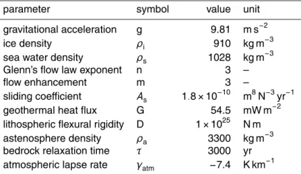
parameter symbol value unit
gravitational acceleration g 9.81 m s−2
ice density ρi 910 kg m−3
sea water density ρs 1028 kg m− 3
Glenn’s flow law exponent n 3 –
flow enhancement m 3 –
sliding coefficient As 1.8×10⁻¹⁰ m8N−3yr−1
geothermal heat flux G 54.5 mW m−2 lithospheric flexural rigidity D 1×1025 N m
astenosphere density ρa 3300 kg m−3
bedrock relaxation time τ 3000 yr atmospheric lapse rate γatm −7.4 K km−1