Vigilância espaço-temporal com superfícies acumuladas

(1)

Tha´ıs Viana Paiva

Vigilˆancia espac¸o-temporal com Superf´ıcies Acumuladas

(2)

Tha´ıs Viana Paiva

Vigilˆancia espac¸o-temporal com Superf´ıcies Acumuladas

Dissertação apresentada como requisito parcial para obtenção de grau de Mestre em Estat´ıstica pela Universidade Federal de Minas Gerais.

Orientador: Prof. Dr. Renato Martins Assunc¸˜ao

Programa deP ós-Graduaç ão emEstat´ıstica Departamento deEstat´ıstica

Instituto deCienciasˆ Exatas UniversidadeFederal deMinasGerais

(3)

Agradecimentos

Agradec¸o primeiramente a Deus por ter me iluminado durante toda a minha caminhada at´e essa conquista.

Aos meus pais Alcy e Beatriz, pelo amor e apoio e por serem meus exemplos a serem seguidos. Devo tudo isso à dedicação de vocês. Ao meu irmão Leandro, pelos momentos de descontração e alegria. Aos meus av ós tão carinhosos, pelos conselhos sábios e experientes. Ao Galletti, pelo amor, compreensão, paciência e tranquilidade.

Ao meu orientador, Professor Renato Assunção, pelas oportunidades, ensinamentos e explica-ç ões durante esses quatro anos, e também por ser o principal motivador para definir o meu destino nos pr óximos quatro anos.

Aos meus professores no curso de Mestrado em Estat´ıstica, pelo conhecimento e convivência durante esse per´ıodo. Aos funcionários da secretaria de Estat´ıstica da UFMG e à FAPEMIG pelo apoio financeiro.

Aos amigos e amigas do Leste, em especial a Érica, Aline, Márcia, Let´ıcia, Gabi e Alessandra, por tanta ajuda e apoio e por escutarem todas as minhas reclamações e hist órias. Às amigas do bonde, Ju, Naty, Bárbara, Joana, Suelen e Taci, e às amigas eternas, Amanda, Amanda, Iara e Ana Luisa, pelos momentos de diversão e conversas intermináveis. A todos os amigos e familiares que de alguma maneira contribuiram para a realização desse trabalho. Muito Obrigada!

(4)

Resumo

O mapeamento de crimes e doenças fornece informações sobre o padrão espacial e temporal de ocorrência dos eventos. É de interesse o monitoramento dos eventos para a detecção precoce de mudanças no seu padrão espacial. Esta dissertação apresenta um método de vigilância espaço-temporal prospectiva de dados pontuais, verificando se há um cluster emergente. A cada novo evento, o escore local de Knox é calculado e suavizado de maneira a formar uma superf´ıcie estocástica. Essas superf´ıcies são então acumuladas sequencialmente até que ultrapassem um limiar estabelecido, quando o alarme soa, identificando a região do provável cluster. As vantagens estão em exigir pouca informação prévia do usuário e em fornecer uma maneira de identificar a localização de poss´ıveis clusters, através da visualização da superf´ıcie acumulada. A performance do método foi avaliada a partir de resultados de simulações em diferentes cenários. O método foi aplicado a um conjunto de dados de casos de meningite em Belo Horizonte.

Palavras-chaves: Sistema de Vigilˆancia, Dados Pontuais, Espac¸o-Temporal, Escore de Knox Local,

Su-perf´ıcies Acumuladas.

(5)

Abstract

Mapping crime and disease events provides information about the spatial and the temporal pattern of these events. To guide actions based on such information, it is necessary to use a statistical method to identify when there is a change in the pattern of events. We developed a space-time prospective surveillance method when the data are point events, monitoring if there is an emerging cluster. At each new event, a local Knox score is calculated and spatially spread to form a stochastic surface. The surfaces are accumulated sequentially until it overcomes a specified threshold, when an alarm goes off, identifying the region of the probable cluster. The advantages are to require little prior knowledge from the user and to provide a way to identify the locations of the possible clusters, through the visualization of the cumulative surface. A simulation study is presented for different scenarios and a dataset of meningitis cases in Belo Horizonte was monitored.

Keywords: Surveillance, Point Pattern, Space-Time, Local Knox Score, Cumulative Surfaces.

(6)

Sum´ario

Lista de Figuras v

Lista de Tabelas vii

1 Introduc¸˜ao 1

1.1 Objetivos . . . 4

1.2 Organizac¸˜ao do Trabalho . . . 4

2 Prospective space-time surveillance 5 2.1 Introduction . . . 5

2.2 Review of the local Knox method . . . 7

2.3 Methodology . . . 11

2.3.1 Cumulative Surfaces . . . 11

2.3.2 Determining the thresholdh. . . 13

2.3.3 Overview of the surveillance method . . . 17

2.4 Simulations . . . 18

2.4.1 Scenario without clusters . . . 20

2.4.2 Scenario with clusters . . . 22

2.4.3 Scenario with cluster - Non-homogeneous Poisson Process . . . 29

2.5 Application . . . 32

2.6 Discussion . . . 36

Referˆencias Bibliogr´aficas 37

(7)

Lista de Figuras

1.1 Visualizac¸˜ao da superf´ıcie acumulada em n´ıveis de contorno, para os casos de meningite . . . 3

2.1 View of the neighborhood ofi-th event . . . . 10

2.2 Three-dimensional visualization of the score zi and its respective surface, for a

random set of points . . . 12

2.3 Time series of the scoresz+_i obtained in an illustrative example . . . 13

2.4 QQ-Plot of the theoretical quantiles of the Gumbel distribution versus the observed quantiles of the maxima of the surfaces, in an illustrative example . . . 16

2.5 Histogram of the maxima of the surfaces, with the Gumbel density and the thresh-olds highlighted, in an illustrative example . . . 16

2.6 View of the coordinates of events generated in the scenario without cluster . . . 20

2.7 Comparative graphs of empirical and theoretical thresholds, for the scenario without clusters . . . 21

2.8 View of the events’ coordinates generated in the scenario with clusters with different intensities . . . 23

2.9 Comparative graphs of empirical and theoretical thresholds, for the clusters with different intensities . . . 23

2.10 View of the events’ coordinates generated in the scenario with clusters with different extents . . . 25

2.11 Comparative graphs of empirical and theoretical thresholds, for the clusters with different extents . . . 26

(8)

LISTA DE FIGURAS vi

2.12 View of the events’ coordinates generated in the scenario with clusters with different shapes . . . 28

2.13 Comparative graphs of empirical and theoretical thresholds, for the clusters with different shapes . . . 29

2.14 View of the events’ coordinates generated in the scenario with clusters, with the events distributed according to a homogeneous and a non-homogeneous Poisson process . . . 30

2.15 Comparative graphs of empirical and theoretical thresholds, in the scenarios with homogeneous and non-homogeneous Poisson process . . . 31

2.16 Spatial coordinates of the meningitis cases in Belo Horizonte . . . 32

2.17 View of a surfacewi(x,y), with the spatial coordinates of the meningitis cases in Belo

Horizonte . . . 33

2.18 Histogram of the maxima of the cumulative surfaces obtained in the permutations, for the meningitis cases . . . 33

2.19 Cumulative surface at the moment that the alarm sounded, for the meningitis cases 34

2.20 View of the cumulative surface in contour levels, for the meningitis cases . . . 34

2.21 Time series of theziscores, of the meningitis cases . . . 35

(9)

Lista de Tabelas

2.1 Results of the scenario without cluster: (a) surveillance for all events; (b) surveillance for the last 100 events . . . 21

2.2 Results in the scenario with cluster, with different intensities: (a) cluster with 10 events; (b) cluster with 25 events; (c) cluster with 50 events . . . 24

2.3 Results in the scenario with cluster, with different cluster extents: (a) cluster in region [5,5.5]2 ×[9,10]; (b) cluster in region [5,6]2 ×[9,10]; (c) cluster in region [4,7]2×[9,10] . . . 27

2.4 Results in the scenario with cluster, with different shapes: (a) square cluster in region [5,6]2_{; (b) rectangular cluster in region [5,}_5.25]_×_[3,_{7] . . . .} ₂₉

2.5 Results in the scenario with cluster: (a) events distributed according to a homo-geneous Poisson process, (b) events distributed according to a non-homohomo-geneous Poisson process . . . 31

(10)

Cap´ıtulo 1

Introduc¸˜ao

A consideração simultânea dos padr ões espaciais e temporais da ocorrência dos eventos é importante para identificar clusters ou conglomerados espaço-temporais. Definimos um cluster espaço-temporal como uma região geograficamente pequena em relação à região em estudo e que concentra um n úmero excessivo de eventos durante um per´ıodo limitado de tempo.

Os métodos de detecção de clusters espaço-temporais são, em sua maioria, retrospectivos. Esses métodos procuram por evidências da presença de um cluster em um banco de dados de eventos já ocorridos. O teste de detecção de conglomerados espaço-temporais mais popular foi desenvolvido por Knox (1964), e ele testa se há interação espaço-temporal. Ou seja, ele testa se casos pr óximos no espaço tendem a estar próximos no tempo também. Mantel (1967) estendeu o teste de Knox, usando as distâncias espaciais e temporais entre os pares de eventos ao invés dos indicadores binários de proximidade. Jacquez (1996) propôs um teste para interação espaço-temporal dek vizinhos mais pr óximos e compara os resultados com os testes de Knox e Mantel, mostrando que o seu teste tem maior poder que os outros. Esses três testes podem ser viciados se a população de risco subjacente muda diferencialmente. Kulldorff(1999) prop ôs uma modificação para solucionar esse problema, mas ela exige informação da população sob risco.

Ao analisar eventos como crimes e doenças, um objetivo importante é detectar um cluster emergente, através da vigilância prospectiva. O desafio é desenvolver métodos de vigilância eficientes e que detectem rapidamente os clusters, além de minimizar o n úmero de alarmes falsos. O interesse é focado em aç ões que possam mitigar os efeitos dos clusters se realizadas rapidamente. Recentemente, pode-se observar um grande desenvolvimento de métodos prospectivos pu-ramente temporais, especialmente na área epidemiol ógica. Os métodos mais usados para fazer vigilância prospectiva epidemiol ógica foram resumidos e avaliados em Sonesson and Bock (2003).

(11)

CAPÍTULO 1. INTRODUÇ ÃO 2

H öhle (2007) desenvolveu um pacote para o software R para fazer a vigilância prospectiva para dados epidemiol ógicos.

Poucos métodos para vigilância prospectiva espaço-temporal foram desenvolvidos até o mo-mento. Um desses métodos foi apresentado por Kulldorff (2001) e calcula uma estat´ıstica de scan espaço-temporal contando o n úmero de eventos dentro de um cilindro de raio e altura pré-estabelecidos. Neill et al. (2005) também desenvolveram um método de detecção de clusters emergentes usando a estat´ıstica de scan espaço-temporal. Uma extensão do método de scan foi proposto por Kulldorffet al. (2005), que não precisa de informaç ões sobre a população em risco. Estes métodos são baseados em idéias de testes de hip óteses, que não são adequados no contexto de vigilância prospectiva (Woodall et al., 2008). Rodeiro and Lawson (2006) utilizam modelos Baye-sianos espaço-temporais para detectar um aumento do risco em mapas de doenças com dados de áreas. Diggle et al. (2005) também apresentam um modelo de vigilância para processos pontuais, monitorando se probabilidades preditivas, determinadas espacial e temporalmente, ultrapassam um limiar pré-estabelecido. A principal desvantagem desses métodos é que eles exigem muito do usuário em termos de modelagem estocástica e podem ter um custo computacional elevado ao se fazer vigilância espaço-temporal, já que é necessário reajustar o modelo à medida que novos eventos ocorrem.

Rogerson (2001) combina a estat´ıstica de Knox sob uma perspectiva local com somas acumu-ladas, de forma a detectar onde e quando ocorre uma interação espaço-temporal. Esse método, usando a estat´ıstica de Knox local, foi avaliado por Marshall et al. (2007), comparando os efeitos dos parâmetros e dos dados nos resultados, e observou-se que o método de Rogerson não teve um bom desempenho na detecção de clusters. Um método mais recente de vigilância prospectiva espaço-temporal é proposto por Assunção and Correa (2009), que utilizam martingales para fazer a vigilância de dados pontuais. Uma desvantagem desse método é assumir um cluster de formato espacial circular.

(12)

para a abordagem prospectiva e serão apresentadas neste trabalho. O escore local é distribu´ıdo no espaço através de uma densidade de kernel, formando uma superf´ıcie estocástica. As superf´ıcies são acumuladas sequencialmente à medida que os eventos ocorrem. Os picos dessas superf´ıcies identificam áreas que presenciaram recentemente um n úmero de eventos maior que o esperado. Se a superf´ıcie acumulada ultrapassar um limiar determinado, um alarme é soado e, um ou mais clusters localizados são identificados.

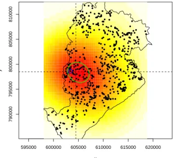
Com a utilização das superf´ıcies é poss´ıvel identificar os locais dos poss´ıveis clusters no mo-mento em que o alarme soa. Também é poss´ıvel visualizar os n´ıveis de interação espaço-temporal em toda a região, e captar a emergência de clusters de diferentes formatos. Analisando-se os valores dos escores locais de cada evento, também é poss´ıvel determinar quais eventos provém do cluster. Na Figura 1.1, podemos ver o resultado da aplicação do método para dados de meningite em Belo Horizonte. O gráfico apresenta a superf´ıcie acumulada até o momento em que o alarme soou, com os eventos que foram registrados e a região do poss´ıvel cluster destacada.

595000 600000 605000 610000 615000 620000

790000

795000

800000

805000

810000

x

y

Figura 1.1: Visualizac¸˜ao da superf´ıcie acumulada em n´ıveis de contorno, para os casos de meningite

(13)

1.1 Objetivos

O objetivo desta dissertação é a apresentação do método desenvolvido de vigilância espaço-temporal com superf´ıcies acumuladas, juntamente com as fórmulas corrigidas para a abordagem prospectiva, bem como avaliar a performance do método a partir de resultados de simulações e a aplicação a um banco de dados.

1.2 Organizac¸˜ao do Trabalho

(14)

Cap´ıtulo 2

Prospective space-time surveillance with geographical

iden-tification of the emerging cluster

2.1 Introduction

The simultaneous consideration of spatial and temporal patterns of occurrence of events is important to identify spatial-temporal clusters. We define a spatial-temporal cluster as a region geographically small in relation to the study area and concentrating an excessive number of events in a limited period of time.

The methods for detecting spatial-temporal clusters are mostly retrospective. These methods look for evidence of the presence of a cluster in a database of events that have already occurred. The interest is to understand the process that generated the events, and identify potential risk factors. The most popular test to detect spatial-temporal clusters was developed by Knox (1964). It tests if there is space-time interaction. That is, it tests whether cases near each other in space tend to be close in time as well. The Knox test is based on the number of pairs of events that are simultaneously close in space and time, with proximity being defined as a binary indicator variable based on numerical thresholds. Mantel (1967) extended the Knox test, using the spatial and temporal distances between pairs of events instead of binary indicators of proximity. Jacquez (1996) proposed a test for space-time interaction of the k nearest neighbors and compared the results with the Knox and Mantel tests, showing that his test had a greater power. The problem is that these three tests can be biased if the underlying population at risk changes differentially. Kulldorff(1999) proposed a modification to the Knox test to fix this problem, with a drawback of requiring information about the underlying population.

(15)

CAP´ITULO 2. PROSPECTIVE SPACE-TIME SURVEILLANCE 6

When dealing with events such as crimes and diseases, an important goal is to detect an emerg-ing cluster through prospective surveillance. The challenge is to develop efficient surveillance methods that rapidly detect clusters as soon as possible after their emergence, while controlling the number of false alarms. The interest is focused on actions that can mitigate the effects of the clusters if they are performed quickly enough.

There is a large number of purely temporal prospective methods, especially in epidemiol-ogy. The methods most used to make epidemiological prospective surveillance are summarized and evaluated in Sonesson and Bock (2003). H¨ohle (2007) developed a package for R to make epidemiological prospective surveillance.

Very few spatial-temporal prospective surveillance methods have been developed so far. One method was presented by Kulldorff(2001) and it calculates a space-time scan statistic counting the number of events within a cylinder of radius and height pre-established. Neill et al. (2005) also developed a method to detect emerging clusters using a space-time scan statistic. An extension for the scan method was proposed by Kulldorffet al. (2005), which does not require information about the population at risk. However, these methods are based on ideas of hypothesis testing, which are not appropriate in the context of prospective surveillance (Woodall et al., 2008). Rodeiro and Lawson (2006) used spatial-temporal Bayesian models to detect an increase in disease risk on maps with data areas. Diggle et al. (2005) also present a model to monitor point process, predicting spa-tially and temporally localised excursions over a pre-specified threshold. The main disadvantage of these methods is that they require a lot from the user regarding stochastic modelling and they can have a high computational cost when making space-time surveillance, since it is necessary to refit the model when new data arrive.

Rogerson (2001) combines the Knox statistic under a local perspective with accumulated sums in order to detect when a space-time cluster is emerging. This method, using the local Knox statistic defined by Rogerson (2001), was evaluated by Marshall et al. (2007). They compared the effects of parameters and data on the results, and concluded that the method of Rogerson did not have a satisfactory performance. A more recent prospective spatial-temporal surveillance method is proposed by Assunc¸˜ao and Correa (2009), using a martingale approach to monitor point patterns. The disadvantage of this method is that it assumes a spatially circular shaped cluster.

(16)

the prospective detection of clusters of space-time point patterns. For every new event that occurs, it is calculated a local Knox score, with the definition from Rogerson (2001) modified. This local score takes into account the number of events close in space and time. This local score is distributed in the space through a kernel density, forming a stochastic surface. The surfaces are accumulated sequentially as the events occur. The peaks of these surfaces identify areas where a number of events greater than expected recently happened. If the surface exceeds a certain threshold, an alarm is sounded, and one or more localized clusters are identified.

There are several advantages of using surfaces. In contrast with other methods of surveillance, it is possible to identify the locations of probable clusters, not only to signal its emergence. Using surfaces also enables to visualize the levels of space-time interaction all over the study region, and capture the emergence of clusters with different shapes. Analyzing the scores for each event, it is also possible to determine which events comes from the cluster.

Furthermore, the methodology is based on sequential inferencial procedures, unlike other methods, such as Kulldorff(2001) based on hypothesis testing. With this we avoid the problem of controlling multiple successive tests.

Another very important advantage of our methodology is that it does not require prior mod-eling of the spatial and temporal patterns of data. This makes the method accessible to users with little statistical knowledge, so it can be used directly by public agencies responsible to take necessary actions in the occurrence of a cluster.

2.2 Review of the local Knox method

Rogerson (2001) defined a local Knox statistic, decomposing the global measure of space-time interaction developed by Knox (1964) into local scores associated with each individual event. For each pair of events, we will define a dummy variable indicating if the two events are at a distance smaller than a critical space radiusrs. Following the notation of Rogerson (2001), letnsbe the total

number of pairs of events close in space. Similarly, we will define a binary variable indicating that the waiting time between two events is smaller than a critical timertand letntbe the total number

of such pairs. We will denote bynstthe total number of pairs of events that are close in space and

time. The test of Knox (1964) is based on this statistic.

(17)

in time and close in space and time from thei-th event, respectively, withi= 1, . . . ,n. The Knox statisticnstcan be decomposed in terms of local statisticsnst(i), sincenst=1/2Pn_i=1nst(i).

The local Knox score defined by Rogerson (2001) is:

zi = nst(i)

−E{Nst(i)} −0.5

p

Var{Nst(i)}

(2.1)

whereNst(i) is the random variable associated with the observed valuenst(i). To determine the

null distribution ofNst(i), Rogerson (2001) assumes that each random permutation of the times,

keeping the spatial coordinates fixed, is equally likely. He also considers that thei-th event can be any of thenevents observed, and his time is also permuted. So, the locationican be assigned to any of the times fromj=1, . . . ,n. The resulting distribution is a weighted sum of hypergeometric distributions, each one corresponding to the times that can be assigned to locationi. With this, he obtained:

E{Nst(i)}= 2ntns(i)

n(n−1) (2.2)

Var{Nst(i)}=

h

2(n−1)nt−Pnj=1nt(j)2

i

ns(i) (n−1−ns(i))

n(n−1)2_(n₋₂₎ (2.3)

Sim ões and Assunção (2005) and Marshall et al. (2007) found that (2.3), the variance proposed by Rogerson, was inaccurate and corrected it:

Var{Nst(i)} =

        n X

j=1

nt(j)2

       

ns(i)

n(n−1)2

"

−(n−1−ns(i)) n−2 +ns(i)

# +      

2ntns(i)

n(n−1)

n−1−ns(i)

n−2 −

2ntns(i)

n(n−1)

!2      =      2(n

−1)nt− n

P

j=1

nt(j)2

     ns(i) (n

−1−ns(i))

n(n−1)2_(n₋₂₎ +

ns(i)2 n

P

j=1

nt(j)−2nt

n

2

n(n−1)2 (2.4)

(18)

However, there is a serious problem in using these local scores in a prospective method. Since the goal is to make prospective surveillance, we are interested in measuring the local space-time interaction as each new event occurs. The statisticnst(i) is calculated for each new event that arises

and, at this moment, there are only those events that happened before the event in question. Future events have not occurred yet and can not be used in the calculation ofnst(i).

As defined by Rogerson (2001), the local scores are suitable for detection of clusters in retro-spective analysis, but are not appropriate for a proretro-spective use. The computation ofnst(i) in (2.2)

considers as possible neighbors of thei-th event both the events that occurred before thei-th, and those that occurred later. Consequently, the calculation of moments is not done correctly. This explains the disappointing results of the prospective Rogerson method found by Marshall et al. (2007). If the local score is defined appropriately under the prospective context, as explained ahead, the Rogerson method presents a very good performance (Piroutek, Assunc¸˜ao, and Paiva, 2010).

To correct the Rogerson method, we consider that thei-th event is the last one, so there are no events with times greater than it. We will defineN_st∗(i) as the random variable of the number of events close in space and time of thei-th event, considering only the events that happened before it. It is also necessary to define:

n∗s(i) number of events that are close in space of thei-th event, considering only those events that happened before it;

n∗_t(i) number of events that are close in time of thei-th event, considering only those events that happened before it;

n∗_st(i) number of events that are close simultaneously in space and time of thei-th event, considering only those events that happened before it;

To find the null distribution ofN∗_st(i), we permute the observed times across the spatial coor-dinates, but now we will keep the i-th event fixed. The resulting distribution will be only one hypergeometric distribution, instead of the weigthed sum of Rogerson (2001).

(19)

of thei-th event, and the remaining ones are of type B. So we will have a total of (i−1) arrows, of whichn∗_t(i) are of type A. We take a sample of sizen∗s(i) from the (i−1) arrows to distribute among

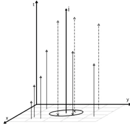
the events that happened close in the space of thei-th event. Figure 2.1 is an example of a set of points, with the spatial coordinates represented in the horizontal axis and the times of occurrence of the events represented on the vertical axis, with the time of the i-th event highlighted. The dotted arrows represent the events of type A, those who are close in time of thei-th event. The events with the locations within the circle are those who are neighbors in space of thei-th event.

y

x

t

i

Figure 2.1: View of the neighborhood ofi-th event

Hence,N∗_st(i) follows a hypergeometric distribution with parameters (i−1),n∗_t(i) en∗s(i). That is,

PnN_st∗(i)=ko= n∗

t(i) k

i−1−n∗_t(i)

n∗ s(i)−k

i−1

n∗ s(i)

The mean and the variance ofN_st∗(i) are given by:

EnN∗_st(i)o= n

∗

s(i)n∗t(i)

i−1 (2.5)

VarnN∗_st(i)o= n

∗

s(i)n∗t(i)(i−1−n

∗

s(i))(i−1−n∗t(i))

(i−2)(i−1)2 (2.6)

It is not possible to compare the variances (2.4) and (2.6), since they are based innst(i) en∗_st(i),

(20)

2.3 Methodology

2.3.1 Cumulative Surfaces

The Cumulative Surface method is based on the local Knox scores defined in (2.1), with mean and variance given by (2.5) and (2.6), respectively. For each event, it is counted the number of events that are close to him in space and that happened a little earlier in time. The local Knox score is then calculated by standardizing this number according to (2.1).

The score is spread around the position of the i-th event through a two-dimensional kernel function. The function used in the method is the bivariate Gaussian density function defined as:

K∗(x,y)= 1

2πexp

−1 2(x

2₊_y2₎ _(2.7)

The kernel functions modify the functions K∗(x,y), transferring them to a new center and changing its concavity with the bandwidth parameterτ. Namely, the positiveziscores are spread

around the coordinates (xi,yi) of thei-th event, forming surfaceswi(x,y) given by:

wi(x,y)=z+_i Ki(x,y)=

z+_i τ2K

∗x−xi

τ ,

y−yi

τ

(2.8)

wherez+_i =max{0,zi}.

Note that

x

wi(x,y)dxdy=z+_i

To form the surface of thei-th event denoted bywi, the region is divided into a grid with size

specified. This grid is determined by dividing the range of the events on the axisx andyin the size established. Coordinates (x,y) are then the points of the grid where the surface is calculated.

At the point (xi,yi) the surface has its maximum values equal towi(xi,yi) = z+_iK∗(0,0)/τ2 =

z+_i /2πτ2. As the distance between the grid point (x,y) and the event coordinates (x_i,y_i) increase,

K∗(x,y) becomes 1/2πmultiplied by a value between 0 and 1 getting smaller. The value of the

surface goes to zero for locations away from the event.

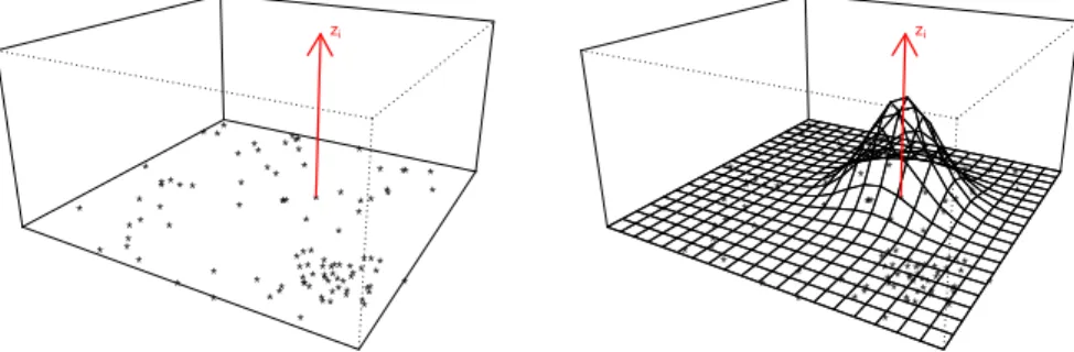
Figure 2.2 shows, for a random set of points, how the scorez+

i is spread around its position,

(21)

CAP´ITULO 2. PROSPECTIVE SPACE-TIME SURVEILLANCE 12 * * * _* * * * * * * * * * * * * * * * * * * * * * * * * * * * * * * * * * * ** * * * * * * * * * * * * * * * * * * * * * * * * * ** * * * * * * * * * ** * * * * * ** * *** * * * * * * * * * * * zi * * * _* * * * * * * * * * * * * * * * * * * * * * * * * * * * * * * * * * * ** * * * * * * * * * * * * * * * * * * * * * * * * * ** * * * * * * * * * ** * * * * * ** * *** * * * * * * * * * * * zi

Figure 2.2: Three-dimensional visualization of the scorezi and its respective surface, for a random set of

points

The bandwidthτaffects mainly the concavity of the surface. Small values for this parameter make the surface decays rapidly and abruptly, while higher values make the surface decays more slowly.

The bandwidth can be specified as a fixed value in order to get an specific view of the surfaces, if there is knowledge about the range and scale of the data coordinates. Otherwise, the bandwidth value can be estimated automatically. This is done through simulations, generating coordinates uniformly distributed between the minimum and maximum coordinates of the events. At each simulation, it is calculated a value ofτusing the following formula, suggested by H¨ardle (1990) for a random variableZand sample sizen:

τ= 1.06

n1/5 min

(

sd(Z),iqr(Z) 1.34

)

(2.9)

wheresd(Z) is the standard deviation andiqr(Z) is the interquartile range of the variableZ. In our case, the variable Zwill be replaced by the events’ coordinates (x,y), the value of sd(Z) will be the average betweensd(x) andsd(y) and the interquartile rangeiqr(Z) will be the average between iqr(x) andiqr(y). At the end of the simulations, the estimated bandwidth will be the average of the values obtained at each simulation.

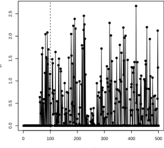
As the scoreszi take into account the information about the neighbors in space and time, we

(22)

[0,10]×[0,10] and times also uniformly distributed in [0,10]. In this case, a value of them∗window equal to or greater than 100 would be enough for the escores to stabilize.

events

zi

0 100 200 300 400 500

0.0

0.5

1.0

1.5

2.0

2.5

Figure 2.3:Time series of the scoresz+_i obtained in an illustrative example

We also define another windowm∗as the number of surfaces of events prior to thei-th event that are going to be accumulated. This window is defined because the oldest events do not help to detect an emerging cluster, causing only a noise in the variance.

At eachi-th event, we accumulated iteratively the lastm∗surfaceswj(x,y):

Si(x,y) = i

X

j=i−m∗₊₁

wj

= Si−1(x,y)−wi−m∗(x,y)+z+

iKi(x,y) withi=1,2, . . . ,n. (2.10)

2.3.2 Determining the thresholdh

The threshold h must be determined as a value of the distribution of the maxima of the cumulative surfaces, such that it is under control the false alarm probability. As we are looking at the maxima of stochastic surfaces that are accumulated over time, it is not immediate how to find a theoretical distribution to determine the thresholdh. However, we use two approaches to find this value, using in both the maxima of the maxima of the surfaces maxi{max(x,y)Si(x,y)}obtained

by permutations of the events’ times.

Let us define one more windowm∗∗ as the number of successive accumulated surfacesSi(x,y),

(23)

surfaces corresponding to the lastm∗∗events, that isi=n−m∗∗+1, . . . ,n.

Controlling the probability of false alarms with the windowm∗∗corresponds to determine the ARL, Average Run Length. It is the expected number of events to happen until the alarm goes off

falsely, used in other surveillance methods like Rogerson (2001) and Assunc¸˜ao and Correa (2009). The first step in the method is to test if the number of events in a training dataset is greater than or equal to the sum of the three windows, i.e.

n≥m+m∗+m∗∗

If this condition is met, then the data set is large enough so that the scoresziare stable and we

can use the windowsm∗andm∗∗.

At each permutation, the spatial positions are kept fixed and times are permuted. That is, we generate new configurations of events under the assumption that there is no space-time interaction. These simulated configurations follow the purely spatial and purely temporal pattern of the data. The surfaces are then accumulated and the maxima of the maxima of the surfaces of the lastm∗∗ events are stored. From now on, we will refer to the these values as the maxima of the surfaces.

In the first approach, we fit a Gumbel distribution to the maxima of the surfaces, and the threshold hteo is the value obtained through its distribution function. The reason for this is a

theorem of Piterbarg (1996). In the second approach, the thresholdhempis obtained as the percentile

of the empirical distribution function of the maxima. We detail below the two approaches.

Theoretical threshold

The stochastic process{S(x), x∈T}, whereT⊂Rk_and_x_∈_T_{represents a location, is a Gaussian}

field if, for any k ≥ 1 and any locations x1, . . . ,xk ∈ T, the vector (S(x1), . . . ,S(xk))T is normally

distributed (Rue and Held, 2005). LetS(x), withx ∈ Rn_{, be a homogeneous Gaussian field - i.e.,}

with constant moments over the region - with zero mean, covariance functionρ(x)=R

ke

ikx_Ψ₍_k_)d_k_, ρ(0)=σ2, and spectrumΨ(k).

(24)

direction of the propagation. In this case, let the unit volume be|V|=λ0λc, whereλ0is the mean

wavelength andλcthe mean crest length. That is, the unit volume is the mean volume that a wave

occupies.

Piterbarg’s theorem (1996, Theorem 14.1) determines the asymptotic extreme value distribution for the maximum of a Gaussian homogeneous field inRn_{. Let}_T_{be the subset}_T_⊂Rn_{with volume}

|T|, or with sizeN=|T|/|V|, where|V|is the unit volume defined above. According to the theorem, we have:

P

max

x∈T S(x)≤σu

∼exph−(2π)n−21e−u2/2H_n₋₁(u)Ni (2.11)

where Hn are Hermite polynomials with respect to the standard Gaussian density (H0(u) = 1,

H1(u) = u,H2(u) =u2−1, . . .). WhenNincreases, i.e. the number of waves within the subsetT

increases, the distribution tends asymptotically to a Gumbel distribution:

G(u)=exp −exp (−a(u−u0)) (2.12)

whereu0≈x0+

(n−1) log(x0)

x0 ,a

=u0− (n

−1)

u0 , andx0

= p2 logN+(n−1) log(2π).

In our case, we are considering the cumulative surface as the homogeneous Gaussian field as of thei-th event. To apply the approximation (2.12), we needN, the expected number of waves in the subsetT, which is not simple to calculate in our method. Thus, we use a theoretical approximation to the distribution of the maxima of the surfaces to determine the thresholdh.

Let us consider a Gumbel distribution with parametersαandβ, with the following density and distribution functions:

f(x)= 1

βexp

(

−(x−µ) β

)

exp

(

−exp

"

−(x−µ) β

#)

(2.13)

F(x)=exp

(

−exp

"

−(x−µ) β

#)

(2.14)

To verify the adequacy of our assumption about the Gumbel distribution, we analyzed the maxima of the maxima of the cumulative surfaces maxi{max(x,y)Si(x,y)}, obtained from 1000

(25)

statistics of the maxima of the maxima of the surfaces, obtained from 1000 permutations, and in the horizontal axis the theoretical quantiles of a standard Gumbel distribution, with parameters µ=0 andβ=1.

−2 0 2 4 6

50

100

150

200

theoretical quantiles

sample quantiles

Figure 2.4: QQ-Plot of the theoretical quantiles of the Gumbel distribution versus the observed quantiles of the maxima of the surfaces, in an illustrative example

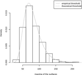
maxima of the surfaces

Density

50 100 150 200

0.000

0.005

0.010

0.015

empirical threshold theoretical threshold

Figure 2.5: Histogram of the maxima of the sur-faces, with the Gumbel density and the thresh-olds highlighted, in an illustrative example

Since the points plotted in the QQ-Plot of Figure 2.4 are very close to a straight line, one can consider that the observed and theoretical quantiles are linearly related. This suggests that, in the scenario where there is no space-time interaction, the observed values seems to follow a Gumbel distribution with different parameters of location and scale. As we will use this distribution of the maxima of the surfaces to find a thresholdhteo under the null hypothesis, it is sufficient to check

that this approximation is valid in this scenario.

The maximum likelihood estimators of the parametersµandβof the maxima’s distribution can not be found analytically. We find them numerically, with initial values obtained by the method of moments. With ˆµand ˆβ, we can determine, from the distribution function (2.14), the threshold hteo as the value such that the probability that at least one of the last m∗∗ cumulative surfaces

(26)

the probability of false alarm.

P max

x,y {Sn−m

∗∗₊₁(x,y)}>h_teo or max x,y {Sn−m

∗∗₊₂(x,y)}>h_teo or

. . . or max

x,y {Sn(x,y)}>hteo

!

=1−F(hteo)=1−exp

(

−exp

"

−(hteo−µ)ˆ ˆ β

#)

=α (2.15)

In Figure 2.5, we see how the density of a Gumbel distribution with parameters ˆµand ˆβ fits well the histogram of the maxima of the cumulative surfaces found in 1000 permutations under the assumption that there are no clusters. Moreover, we can see that the threshold valueshteoand

hemp, which will be described in the next section, are very close.

Empirical threshold

To determine the thresholdhemp, we will use again the windowm∗∗ to control the probability

of false alarm. A thresholdhis determined in order that the probability that at least one of the last m∗∗_{surfaces’ maxima is higher than}_h_{is equal to}_{α. This is the probability of a false alarm, given} by

P max

x,y {Sn−m

∗∗₊₁(x,y)}>h_emp or max x,y {Sn−m

∗∗₊₂(x,y)}>h_emp or

. . . or max

x,y {Sn(x,y)}>hemp

!

= α (2.16)

At the end of B random permutations of the events’ times, we have B maxima of surfaces’ maxima. The thresholdhempis the (1−α)-th percentile of the maxima distribution.

It is important to note that, since that we are observing maxima of surfaces, we are dealing with a very asymmetric distribution with heavy tail. Because of that, a sample percentile may not be adequate to estimate a theoretical percentile, if the sample size is not large enough.

2.3.3 Overview of the surveillance method

The cumulative surface method was implemented in C language, divided in two parts. The first part uses a training dataset to make the times’ permutations and determine the threshold value. Then, this value is used in the second part, where the surveillance is made.

(27)

bandwidthτ, and the grid size of the surface. The output is the value of the thresholdshteoehemp.

For a dataset of 500 events, the average running time of this part is 3.5 minutes, in a machine with 2.80 GHz and 2 Gb RAM.

After the thresholdhis determined, it is not necessary to repeat this step when new events are added to the database. Permutations must be done again only if its judged that the overall events’ incidence pattern has changed.

In the second part of the method, the necessary input is the dataset, along with the parameters already fixedm, m∗,m∗∗,rs,rt, α,τand the grid size. In our software, we allow the surveillance

to be run only for the last events in the input dataset. For that, the user specifies the numberaof new events to be monitored. At each new event, the method accumulates the surfaces taking into account the window ofm∗previous events.

Si(x,y) = i

X

j=i−m∗₊₁

wj

= Si−1(x,y)−wi−m∗(x,y)+z+ i Ki(x,y)

withi=n−a+1, . . . ,n. (2.17)

The alarm goes offimmediately after the i-th event if Si(x,y) > hfor some position (x,y). If

this happens, the method outputs the surface accumulated until this moment and thezi values.

With the view of the surface, it is possible to visualize other areas that may also have high levels of space-time interaction. We identify as the locations of possible clusters the regions where the surface was above the thresholdh. With the same computer configuration and 500 events, the average running time of the second part is less than one minute.

The plan for the future is to implement the two parts as an surveillance method in an R package, to allow that it becomes acessible to different users.

2.4 Simulations

(28)

permuting the temporal coordinates 1000 times, keeping the spatial coordinates fixed, as described in Section 2.3.2.

In all scenarios, we use the critical space radiusrsequal to 2 and critical timertequal to 1. Thus,

when data follow a uniform distribution in [0,10]3_{, the expected number of events in the critical}

region is equal to 6.28. The windowsmandm∗∗_{are set equal to 100. These values were determined} proportionally to the total number of events, such that the scores are stabilized and the probability of false alarm is controlled as 0.05 for the lastm∗∗ events. The windowm∗, which corresponds to how many previous events are accumulated to build the surface associated to thei-th event, took the values 10, 25 and 50. In this way, we can analyze its impact on the proportion of false alarms. The grid size to evaluate the continuous surface was set as 50×50. To obtain a better visualization of the surfaces, with distinguishable peaks, the bandwidth was fixed as 0.25.

After determining the threshold valueh, we can proceed to the second part of the surveillance. For each scenario, we ran 1000 simulations. At each simulation, data are generated according to the scenario pattern and the surveillance was carried out.

Let s be the number of total simulations and sA be the number of simulations in which the

alarm went off. LetIC(j) be the indicator variable signing whether the alarm went offcorrectly on

thej-th simulation. It only makes sense when there are clusters, and it indicates if the alarm went offfor a event that belongs to the cluster or occurred near it. Similarly, let IF(j) be the indicator

variable of a false alarm in the j-th simulation. In the scenario without clusters, it indicates the simulations in which the alarm went off. When there are clusters, it indicates the simulations in which the alarm went offfor events before the cluster’s emergence or for events that are far from the cluster’s location. Finally, letdjbe the delay of events that belong to the cluster that occurred

until the alarm went off, in the j-th simulation. With the results of simulations, we will analyze the following measures:

• FAR-False Alarm Rate:

FAR=

Ps

j=1IF(j)

sA

(29)

• AR-Alarm Rate:

AR= sA

s

It is the proportion of simulations in which the alarm went off. When there are no clusters, it corresponds toα, the false alarm probability.

• CED-Conditional Expected Delay:

CED=

Ps

j=1dj IC(j)

Ps

j=1IC(j)

It is the mean number of events from the cluster that happened before the alarm goes off

correctly. When there is no cluster, it is equal to zero.

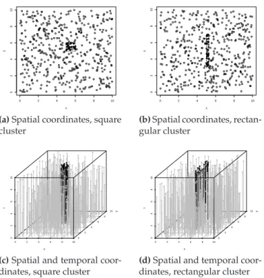
2.4.1 Scenario without clusters

This is the scenario under the null hypothesis, where there is no cluster. Events are generated with the coordinates uniformly distributed in the region [0,10]3. The typical data used to perform the permutations can be seen in Figure 2.6.

0 2 4 6 8 10

0

2

4

6

8

10

x

y

(a)Spatial coordinates

0 2 4 6 8 10

0

2

4

6

8

10

0 2

4 6

8 10

x

y

t

(b)Spatial and temporal coordinates

Figure 2.6: View of the coordinates of events generated in the scenario without cluster

The thresholdshempandhteoare given in Table 2.1(a) and were calculated by using the

permuta-tions and the maxima distribution, respectively. We can also see them in Figure 2.7. The threshold values do not differ much, which means that the results of simulations should be similar forhemp

andhteo.

(30)

Scenario without cluster

m*

h

10 25 50

60

80

100

120

hemp

hteo

Figure 2.7: Comparative graphs of empirical and theoretical thresholds, for the scenario without clusters

the firstm, the window of events needed for the scores’ stabilization. Table 2.1(a) shows the results of the simulations for each value ofm∗. As we are in the scenario without cluster,FARis equal to 1.0 andCEDis equal to 0.0.

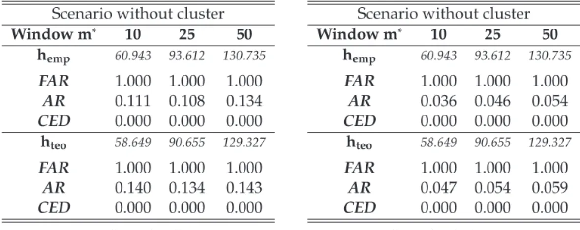
Scenario without cluster

Window m∗ 10 25 50

hemp 60.943 93.612 130.735

FAR _1.000 _1.000 _1.000

AR _0.111 _0.108 _0.134

CED _0.000 _0.000 _0.000

hteo 58.649 90.655 129.327

FAR _1.000 _1.000 _1.000

AR _0.140 _0.134 _0.143

CED _0.000 _0.000 _0.000

(a)Surveillance for all events

Scenario without cluster

Window m∗ 10 25 50

hemp 60.943 93.612 130.735

FAR _1.000 _1.000 _1.000

AR _0.036 _0.046 _0.054

CED _0.000 _0.000 _0.000

hteo 58.649 90.655 129.327

FAR _1.000 _1.000 _1.000

AR _0.047 _0.054 _0.059

CED _0.000 _0.000 _0.000

(b)Surveillance for the last 100 events

Table 2.1: Results of the scenario without cluster: (a) surveillance for all events; (b) surveillance for the last 100 events

Even under the assumption that there are no clusters, the proportionsARin Table 2.1(a) are larger than α fixed. This is due to the fact that in this case, the surveillance was made for all possible events, i.e. the last 400 events, and the empirical threshold was determined using the last m∗∗=100 events.

(31)

In the results in Table 2.1(b), we see that the proportions are very close to the value set ofα=0.05. Thus, even increasing from 100 to 400 the number of events to be analyzed, the proportion of times the alarm went offdid not increase in the same proportion, staying within the tolerance level αdetermined by user.

2.4.2 Scenario with clusters

In the scenarios with clusters, we generated 500 events. A cluster is formed generating a fixed number of events in a small region of space and a short time interval. The remaining events are generated uniformly distributed in the region [0,10]3. The values of the input parameters were the same as in the previous scenario.

For each scenario with cluster, we analyze the results for three different values of windowm∗=

10, 25 and 50, in order to measure the impact of the choice of this parameter in the results. The simulations were made with the thresholdshempandhteo. In each simulation, the surveillance was

made for all possible events, excluding only the initial windowmfor the scores’ stabilization. The performance of the method was evaluated for different scenarios varying the intensity of the cluster, its size and its format.

Clusters with diff_{erent intensities}

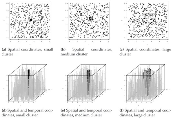
To see the impacts of different cluster intensities, we fixed the cluster region as [5,6]2×[9,10], adding 10, 25 or 50 events besides the underlying uniform intensity. An example of a dataset with the three cluster intensities can be viewed in Figure 2.8.

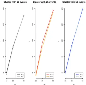
In Table 2.2 we see the thresholdshempandhteofound for each of the values ofm∗. The thresholds

found were very close, as we can see in the graphs of Figure 2.9 confirming the adequacy of the theoretical approach of the maxima distribution described in Section 2.3.2. Therefore, the results with the empirical and the theoretical threshold did not differ much.

Moreover, the thresholds are on the same level for the different intensities of the cluster. This behavior is acoording to the expectations, considering that the presence of a cluster with a different intensity should not change the threshold value.

(32)

0 2 4 6 8 10

0 2 4 6 8 10 x y

(a)Spatial coordinates, cluster

with 10 events

0 2 4 6 8 10

0 2 4 6 8 10 x y

(b)Spatial coordinates, cluster

with 25 events

0 2 4 6 8 10

0 2 4 6 8 10 x y

(c)Spatial coordinates, cluster

with 50 events

0 2 4 6 8 10

0 2 4 6 8 10 0 2 4 6 8 10 x y t

(d)Spatial and temporal

coor-dinates, cluster with 10 events

0 2 4 6 8 10

0 2 4 6 8 10 0 2 4 6 8 10 x y t

(e)Spatial and temporal

0 2 4 6 8 10

0 2 4 6 8 10 0 2 4 6 8 10 x y t

(f)Spatial and temporal

Figure 2.8:View of the events’ coordinates generated in the scenario with clusters with different intensities

Cluster with 10 events

m*

h

10 25 50

60 80 100 120 140 hemp hteo

m*

h

10 25 50

60 80 100 120 140 hemp hteo

m*

h

10 25 50

60 80 100 120 140 hemp hteo

Figure 2.9: Comparative graphs of empirical and theoretical thresholds, for the clusters with different intensities

did not change with the window m∗_{, remaining around eight events. Since we are in a cluster} originally consisted of only 10 events, the alarm sounded around 60% of the time, many of those times falsely.

(33)

Scenario with cluster

Window m∗ 10 25 50

hemp 59.669 92.043 131.408

FAR _0.273 _0.243 _0.282

AR _0.556 _0.600 _0.577

CED _7.953 _7.956 _8.145

hteo 57.693 91.297 131.655

FAR _0.300 _0.257 _0.275

AR _0.603 _0.607 _0.574

CED _7.502 _7.707 _8.036

(a)Cluster with 10 events

Window m∗ 10 25 50

hemp 57.219 97.391 137.832

FAR _0.170 _0.115 _0.103

AR _1.000 _1.000 _1.000

CED _8.997 _9.964 _11.205

hteo 56.204 92.029 135.511

FAR _0.187 _0.137 _0.107

AR _1.000 _1.000 _1.000

CED _8.877 _9.644 _11.113

(b)Cluster with 25 events

Window m∗ 10 25 50

hemp 59.969 94.217 138.982

FAR _0.122 _0.099 _0.078

AR _1.000 _1.000 _1.000

CED _8.641 _9.889 _11.607

hteo 58.278 92.839 140.562

FAR _0.121 _0.114 _0.079

AR _1.000 _1.000 _1.000

CED _8.498 _9.842 _11.661

(c)Cluster with 50 events

Table 2.2:Results in the scenario with cluster, with different intensities: (a) cluster with 10 events; (b) cluster with 25 events; (c) cluster with 50 events

ARwere equal to one, indicating that the alarm sounded in all simulations. As the windowm∗ increases, the false alarm rate decreased, which means that the more information is accumulated, the more the alarm sounds correctly. The mean time expected until the cluster is detected has increased in about one event, with respect to the cluster with 10 events, which means that, pro-portionally, the alarm sounded more quickly. But there is a trade-offbetweenFARandCED, since theCEDincreased directly with the windowm∗. This is due to the fact that accumulating more information, the thresholdhwill increase, decreasing the number of surfaces that would overcome it before the cluster actually starts. Thus, the surface corresponding to the cluster will also take slightly longer to overcome the threshold.

(34)

simulations. The values ofCED have not changed with respect to the scenario with 25 events, again, meaning that the cluster is detected more quickly. We must consider whether the gain in reducingFARis better than the delay of some events when detecting a cluster, according to the type of event and the actions to be taken facing an alarm.

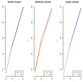
Clusters with diff_{erent extents}

To evaluate the detection power for different cluster extents, we fixed the number of events belonging to the cluster as 25 and vary the spatial region of the cluster as [5,5.5]2, [5,6]2and [4,7]2, while maintaining the temporal coordinates uniformly distributed between [9,10]. The spatial and temporal coordinates of a typical dataset can be viewed in Figure 2.10.

0 2 4 6 8 10

0 2 4 6 8 10 x y

(a) Spatial coordinates, small

cluster

0 2 4 6 8 10

0 2 4 6 8 10 x y

(b) Spatial coordinates,

medium cluster

0 2 4 6 8 10

0 2 4 6 8 10 x y

(c) Spatial coordinates, large

cluster

0 2 4 6 8 10

0 2 4 6 8 10 0 2 4 6 8 10 x y t

coor-dinates, small cluster

0 2 4 6 8 10

0 2 4 6 8 10 0 2 4 6 8 10 x y t

(e)Spatial and temporal

coor-dinates, medium cluster

0 2 4 6 8 10

0 2 4 6 8 10 0 2 4 6 8 10 x y t

(f)Spatial and temporal

coor-dinates, large cluster

Figure 2.10:View of the events’ coordinates generated in the scenario with clusters with different extents

The threshold valueshempandhteo are given in Table 2.3. Observing the graph comparing the

thresholds in Figure 2.11, we see that the threshold values did not change when we are considering clusters spread in a narrower or wider area. These values are also very close to the thresholds found for the previous scenarios.

(35)

Small cluster

m*

h

10 25 50

60

80

100

120

140

hemp

hteo

Medium cluster

m*

h

10 25 50

60

80

100

120

140

hemp

hteo

Large cluster

m*

h

10 25 50

60

80

100

120

140

hemp

hteo

Figure 2.11: Comparative graphs of empirical and theoretical thresholds, for the clusters with different extents

FARof the small cluster were slightly larger than the ones of the medium cluster.

(36)

Window m∗ 10 25 50

hemp 56.499 90.914 138.472

FAR _0.181 _0.157 _0.130

AR _1.000 _1.000 _1.000

CED _8.921 _8.535 _11.246

hteo 56.884 89.900 134.782

FAR _0.174 _0.168 _0.131

AR _1.000 _1.000 _1.000

CED _8.965 _9.488 _11.069

(a)Small cluster

Window m∗ 10 25 50

hemp 57.219 97.391 137.832

FAR _0.170 _0.115 _0.103

AR _1.000 _1.000 _1.000

CED _8.997 _9.964 _11.205

hteo 56.204 92.029 135.511

FAR _0.187 _0.137 _0.107

AR _1.000 _1.000 _1.000

CED _8.877 _9.644 _11.113

(b)Medium cluster

Window m∗ 10 25 50

hemp 54.650 91.582 137.312

FAR _0.212 _0.129 _0.094

AR _1.000 _1.000 _1.000

CED _12.024 _12.846 _14.468

hteo 54.614 90.705 134.889

FAR _0.212 _0.133 _0.101

AR _1.000 _1.000 _1.000

CED _12.019 _12.753 _14.354

(c)Large cluster

Table 2.3: Results in the scenario with cluster, with different cluster extents: (a) cluster in region [5,5.5]2_×

(37)

Clusters with diff_{erent shapes}

As the method uses a cylinder to determine the proximity between events, it is important to examine how the shape of the cluster influences its detection. For this, we compared the results of square-shaped cluster with 25 events in the region [5,6]2with the results of a cluster also with 25 events, but rectangular, in the region [5,5.25]×[3,7]. In both clusters, times are uniformly distributed in [9,10]. The typical dataset can be seen in Figure 2.12.

0 2 4 6 8 10

0 2 4 6 8 10 x y

(a)Spatial coordinates, square

cluster

0 2 4 6 8 10

0 2 4 6 8 10 x y

(b)Spatial coordinates,

rectan-gular cluster

0 2 4 6 8 10

0 2 4 6 8 10 0 2 4 6 8 10 x y t

(c)Spatial and temporal

coor-dinates, square cluster

0 2 4 6 8 10

0 2 4 6 8 10 0 2 4 6 8 10 x y t

coor-dinates, rectangular cluster

Figure 2.12:View of the events’ coordinates generated in the scenario with clusters with different shapes

The threshold values are in Tables 2.4(a) and 2.4(b), together with the results obtained for the two different clusters’ shapes. Again, there was not great difference between the threshold values found, empirically and theoretically, as can be seen in Figure 2.13.

(38)

Squared cluster

m*

h

10 25 50

60

80

100

120

140

hemp

hteo

Straight cluster

m*

h

10 25 50

60

80

100

120

140

hemp

hteo

Figure 2.13: Comparative graphs of empirical and theoretical thresholds, for the clusters with different shapes

Window m∗ 10 25 50

hemp 57.219 97.391 137.832

FAR _0.170 _0.115 _0.103

AR _1.000 _1.000 _1.000

CED _8.997 _9.964 _11.205

hteo 56.204 92.029 135.511

FAR _0.187 _0.137 _0.107

AR _1.000 _1.000 _1.000

CED _8.877 _9.644 _11.113

(a)Square cluster

Window m∗ 10 25 50

hemp 57.246 88.808 138.006

FAR _0.194 _0.195 _0.115

AR _0.999 _1.000 _1.000

CED _11.559 _11.800 _13.787

hteo 57.912 90.012 137.947

FAR _0.173 _0.175 _0.115

AR _0.999 _1.000 _1.000

CED _11.691 _11.886 _13.778

(b)Rectangular cluster

Table 2.4: Results in the scenario with cluster, with different shapes: (a) square cluster in region [5,6]2; (b)

rectangular cluster in region [5,5.25]×[3,7]

2.4.3 Scenario with cluster - Non-homogeneous Poisson Process

To assess if the method is able to identify a true cluster, even if there are different spatial patterns, for example due to the populational density, we generated events with different patterns of occurrence.

With the number of events belonging to the cluster fixed, the other events are generated according to a Non-homogeneous Poisson Process with intensity given by (2.18).

(39)

whereφ(x,y;µ,Σ) is the density function of a bivariate normal distribution at the point (x,y), with meanµ= (µx, µy) and correlation matrixΣ. In this case, we assumed thatµ1 =(3; 7),µ2 = (8; 3),

σ2_x=σ2_y =2 andρ=0.

To form the cluster, we generated 25 events uniformly distributed in the region [5,6]×[5,6] and time between [9,10]. The temporal and spatial coordinates of a typical dataset can be viewed in Figures 2.14(b) and 2.14(d).

0 2 4 6 8 10

0 2 4 6 8 10 x y

(a)Spatial coordinates, HPP

0 2 4 6 8 10

0 2 4 6 8 10 x y

(b)Spatial coordinates, NHPP

0 2 4 6 8 10

0 2 4 6 8 10 0 2 4 6 8 10 x y t

(c)Spatial and temporal

coor-dinates, HPP

0 2 4 6 8 10

0 2 4 6 8 10 0 2 4 6 8 10 x y t

coor-dinates, NHPP

Figure 2.14: View of the events’ coordinates generated in the scenario with clusters, with the events distributed according to a homogeneous and a non-homogeneous Poisson process

The parameters assumed the same values as in the previous scenarios, including the window m∗. To evaluate the results of the scenario with NHPP, they were compared to results obtained in the scenario with the square cluster with 25 events in the region [5,6]2×[9,10], where other events are randomly distributed in the rest of region. Thus, events that do not belong to the cluster follow a Homogeneous Poisson Process with intensityλconstant and equal to 0.475.

(40)

HPP Scenario

m*

h

10 25 50

60

80

100

120

140

hemp

hteo

NHPP Scenario

m*

h

10 25 50

60

80

100

120

140

hemp

hteo

Figure 2.15:Comparative graphs of empirical and theoretical thresholds, in the scenarios with homogeneous and non-homogeneous Poisson process

In Table 2.5, we can see the difference in the results of different scenarios. In both scenarios, the alarm sounded in all simulations. The false alarm rates of NHPP were slightly higher than the rates of HPP, again as expected, since the heterogeneous distribution of the events increase the chance of a random occurrence of a conglomerate of events, not featuring a true cluster. Moreover, the values ofCEDalso increased for the non-homoegeneous scenario, but again it was not a significant change with respect to the performance of the method.

With m∗ 10 25 50

hemp 57.219 97.391 137.832

FAR _0.170 _0.115 _0.103

AR _1.000 _1.000 _1.000

CED _8.997 _9.964 _11.205

hteo 56.204 92.029 135.511

FAR _0.187 _0.137 _0.107

AR _1.000 _1.000 _1.000

CED _8.877 _9.644 _11.113

(a)HPP Cluster

Window m∗ 10 25 50

hemp 61.128 105.788 149.908