Submitted24 May 2016 Accepted 1 November 2016 Published1 December 2016 Corresponding author Erica A.H. Smithwick, [email protected]
Academic editor Christopher Lortie
Additional Information and Declarations can be found on page 18
DOI10.7717/peerj.2745
Copyright 2016 Smithwick et al.
Distributed under
Creative Commons CC-BY 4.0 OPEN ACCESS
Grassland productivity in response to
nutrient additions and herbivory is
scale-dependent
Erica A.H. Smithwick1, Douglas C. Baldwin2and Kusum J. Naithani3
1Department of Geography and Intercollege Graduate Degree Program in Ecology, Pennsylvania
State University, University Park, PA, United States
2Department of Geography, Pennsylvania State University, University Park, PA, United States 3Department of Biological Sciences, University of Arkansas, Fayetteville, AR, United States
ABSTRACT
Vegetation response to nutrient addition can vary across space, yet studies that explicitly incorporate spatial pattern into experimental approaches are rare. To explore whether there are unique spatial scales (grains) at which grass response to nutrients and herbivory is best expressed, we imposed a large (∼3.75 ha) experiment in a South African coastal grassland ecosystem. In two of six 60 × 60 m grassland plots, we imposed a scaled sampling design in which fertilizer was added in replicated sub-plots (1×1 m, 2×2 m, and 4×4 m). The remaining plots either received no additions or were fertilized evenly across the entire area. Three of the six plots were fenced to exclude herbivory. We calculated empirical semivariograms for all plots one year following nutrient additions to determine whether the scale of grass response (biomass and nutrient concentrations) corresponded to the scale of the sub-plot additions and compared these results to reference plots (unfertilized or unscaled) and to plots with and without herbivory. We compared empirical semivariogram parameters to parameters from semivariograms derived from a set of simulated landscapes (neutral models). Empirical semivariograms showed spatial structure in plots that received multi-scaled nutrient additions, particularly at the 2×2 m grain. The level of biomass response was predicted by foliar P concentration and, to a lesser extent, N, with the treatment effect of herbivory having a minimal influence. Neutral models confirmed the length scale of the biomass response and indicated few differences due to herbivory. Overall, we conclude that interpretation of nutrient limitation in grasslands is dependent on the grain used to measure grass response and that herbivory had a secondary effect.
SubjectsAgricultural Science, Conservation Biology, Ecology, Ecosystem Science, Plant Science Keywords Fertilization, Geostatistics, Africa, Spatial autocorrelation, Scale, Autocorrelation, Grassland, Nutrient limitation, Semivariogram, Maximum likelihood
INTRODUCTION
although co-limitation and the role of other nutrients is also acknowledged to be important (Fay et al., 2015). Ecological inference is dependent on the observational scale of the measurements, however, and as such, our ability to infer ecosystem function from patterns in nutrient availability rests on the grain and extent of the measurement (Dungan et al., 2002). In a spatial context, grain reflects the finest level of resolution (precision of measurement) whereas extent refers to the size of the study area, and the choice of these dimensions offer differ among studies (Turner & Gardner, 2015). In the case of nutrient limitation, the optimal grain for diagnosing nutrient limitation, especially in grassland ecosystems, is not known and may vary at fine scales (Klaus et al., 2016). Patchiness in nutrient availability can be governed by variability in soil properties or terrain, spatial variability in microbial community composition, or differential nutrient affinities across functional groups that have different spatial or temporal distributions (Reich et al., 2003;
Ratnam et al., 2008). Perhaps as a result of this spatial heterogeneity, N, P, and N+P limitations on vegetation productivity have all been documented in African savanna or grassland systems (Augustine, McNaughton & Frank, 2003;Craine, Morrow & Stock, 2008;
Okin et al., 2008;Ngatia et al., 2015). This study asks whether new approaches that actively test (sensuMcIntire & Fajardo, 2009) the scale of grass response to nutrients and herbivory can aid understanding of nutrient limitation in grassland ecosystems.
Herbivores influence nutrient availability and can further enhance or diminish spatial and temporal variability in nutrient limitation (Senft et al., 1987;Robertson, Crum & Ellis, 1993;Augustine & Frank, 2001;Okin et al., 2008;Liu et al., 2016). Herbivores affect spatial patterns of nutrient availability directly through deposition of nutrient-rich manure or urine, which can lead to heterogeneous patterns of primary productivity (Fuhlendorf & Smeins, 1999). As animals move across an area and rest in new locations, variability can be further enhanced (Auerswald, Mayer & Schnyder, 2010;Fu et al., 2013). On the other hand, consumption of nutrient-rich grasses may reduce overall variance by reducing differences in biomass amounts compared to ungrazed areas. Through model simulations,
Gil, Jiao & Osenberg (2016)recently showed that herbivores may have a greater influence on controlling biomass at fine versus broad extents, suggesting scale-dependence in herbivore control of plant biomass. In a field experiment, Van der Waal et al. (2016)concluded that herbivore consumption of nutrient rich patches eliminated the positive effects of fertilization on the plant community and that patchiness itself (independent of the patch size) can affect the outcome of trophic relationships in grassland and savanna ecosystems. Taken together, understanding scale dependence (Sandel, 2015), specifically the degree to which grass productivity is governed by the grain and extent nutrient availability and herbivore activity, is important for making inferences about ecosystem function in grasslands and requires new methodological approaches for its study.
any given study, the scale of this autocorrelation structure and its implications for inferring ecological processes are not known in advance. Select studies have employed experimental spatial designs a priori (Stohlgren, Falkner & Schell, 1995) or have used computational simulations to explore the influence of space on ecosystem properties (With & Crist, 1995;Smithwick, Harmon & Domingo, 2003;Jenerette & Wu, 2004). Geostatistical analysis is commonly used (Jackson & Caldwell, 1993b;Robertson, Crum & Ellis, 1993;Smithwick et al., 2005;Jean et al., 2015) to describe the grain and extent of observed ecological patterns, while other approaches may be more useful for predictive modeling of ecological processes through space and time (Miller, Franklin & Aspinall, 2007;Beale et al., 2010), though these, too, rest on an understanding of autocorrelation structures.
Understanding these spatial structures is often elusive because ecological patterns develop from complex interactions among individuals across variable abiotic gradients (Jackson & Caldwell, 1993a;Rietkerk et al., 2000;Ettema & Wardle, 2002) and manifest at multiple spatial scales (Mills et al., 2006). Disturbances further create structural patterns that may influence ecological processes at many scales (Turner et al., 2007;Schoennagel, Smithwick & Turner, 2008). Resultant patchiness in ecological phenomena is common. For example, Rietkerk et al. (2000)observed patchiness in soil moisture at three unique scales (0.5 m, 1.8 m and 2.8 m) in response to herbivore impacts. Following fire in the Greater Yellowstone Ecosystem (Wyoming, USA),Turner et al. (2011)observed variation in soil properties at the level of individual soil cores, andSmithwick et al. (2012)observed autocorrelation in post-fire soil microbial variables that ranged from 1.5 to 10.5 m. Patchiness in soil resources at the level of individual shrubs and trees has been demonstrated by several studies (Liski, 1995;Pennanen et al., 1999;Hibbard et al., 2001;Lechmere-Oertel, Cowling & Kerley, 2005;Dijkstra et al., 2006). In savanna systems, multiple spatial scales are needed to explain complex grass-tree interactions (Mills et al., 2006;Okin et al., 2008;
Wang et al., 2010;Pellegrini, 2016) and it is likely that these factors are nested hierarchically with spatial scale (Pickett, Cadenasso & Benning, 2003;Rogers, 2003;Pellegrini, 2016).
In the absence of understanding the scale at which ecosystems are nutrient-limited, nor the causal mechanisms underlying this scale-dependence, the ability to extrapolate nutrient limitations to broader areas is hindered. Here we report on a study in which we tested the grain-dependence of grass biomass to nutrient additions and herbivory using a novel experimental design. Our objectives were to: (1) quantify the grain size at which vegetation biomass and nutrient concentrations respond to nutrient additions in fenced and unfenced plots, (2) relate the level of biomass response to plant nutrient concentrations and herbivory and (3) assess the degree to which herbivory and nutrient treatments explained the spatial structure of grass productivity through comparison of empirical semivariograms and neutral models (simulated semivariogram models based on prescribed landscape patterns).
soil biogeochemistry (Jackson & Caldwell, 1993a;Rietkerk et al., 2000;Ettema & Wardle, 2002). We posited that, at the finest sampling grain (1×1 m), grass biomass and nutrient concentrations would likely reflect competition for nutrient resources among individuals of a given species, or between occupied and unoccupied (open) locations (Remsburg & Turner, 2006;Horn et al., 2015). At the intermediate grain (2×2 m), we expected that biomass and nutrient concentrations would reflect the outcome of competitive exclusion among grass clumps comprised of different species (Grime, 1973;Schoolmaster, Mittelbach & Gross, 2014;Veldhuis et al., 2016). At the largest grain (4×4 m), we expected that abiotic processes such as variability in hydrology or soil properties would strongly determine the response of grass biomass and nutrient concentrations in addition to competitive processes among individuals and species (Ben Wu & Archer, 2005;Mills et al., 2006). Half of the plots were fenced to exclude herbivory to determine whether there were differences the scale of the response due to animal activity. We used a semivariogram model developed from empirical data and used model parameters to estimate the spatial structure of biomass and nutrient concentrations. We expected that biomass and vegetation nutrient concentrations would have range parameters from empirical semivariograms that corresponded to the hypotenuse distances of the subplot scales (i.e., 1 m, 2.83 m, and 5.66 m hypotenuse distances for the 1×1 m, 2×2 m, and 4 ×4 m subplots, respectively). We expected that patchiness would be highest. i.e., range scales would be smaller, for the unfenced, heterogeneously fertilized plot because these areas would have received nutrient additions in the form of manure and urine from animal activity in addition to nutrient additions (Liu et al., 2016)
For Objective 2, we hypothesized that biomass responses to nutrient additions at the plot level would best explained by foliar N and P concentrations, given previous work indicating the importance of coupled nutrient limitation to grassland productivity (Craine, Morrow & Stock, 2008;Craine & Jackson, 2010;Ostertag, 2010;Fay et al., 2015). We expected that herbivory would have limited effects on biomass productivity relative to the influence of nutrients.
expect to see lower levels of spatial structure explained by the model relative to random processes (higher nugget:sill, described below).
METHODS
Study area
This study was conducted in Mkambathi Nature Reserve, a 7720-ha protected area located at 31◦13′27′′
S and 29◦57′58′′
E along the Wild Coast region of the Eastern Cape Province, South Africa. The Eastern Cape is at the confluence of four major vegetative groupings (Afromontane, Cape, Tongaland-Pondoland, and Karoo-Namib) reflecting biogeographically complex evolutionary histories. It is located within the Maputaland-Pondoland-Albany conservation area, which bridges the coastal forests of Eastern Africa to the north, and the Cape Floristic Region and Succulent Karoo to the south and west. The Maputaland-Pondoland-Albany region is the second richest floristic region in Africa, with over 8,100 species identified (23% endemic), and 1,524 vascular plant genera (39 endemic) (CEPF, 2010) Vegetation in Mkambathi is dominated by coastal sour grassveld ecosystems, which dominate about 80% of the ecosystem (Shackleton et al., 1991;
Kerley, Knight & DeKock, 1995), with small pockets of forest along river gorges, wetland depressions, and coastal dunes. Dominant grasses in the Mkambathi reserve include the coastalThemeda triandra—Centella asiaticagrass community, the tall grassCymbopogon validas—Digitaria natalensiscommunity in drier locations, and the short-grassTristachya leucothrix-Loudetia simplex community (Shackleton, 1990). Grasslands in Mkambathi have high fire frequencies, and typically burn biennially. Soils are generally derived from weathered Natal Group sandstone and are highly acidic and sandy with weak structure and soil moisture holding capacity (Shackleton et al., 1991).
Annual precipitation in Mkambathi Reserve averaged 1,165 mm yr−1between 1925 and 2015 and 1,159 mm yr−1between 2006 and 2015. June is typically the driest month (averaging 30.8 mm 1996–2015) and March is typically the wettest month (averaging 147.6 mm 1996–2015). For nearby Port Edward, South Africa, where data was available, the maximum temperature is highest in February (26.7◦C), averaging 23.7◦C annually, while minimum temperature is coolest in July (average 13.0 ◦C), averaging 17.4 ◦C annually. During the years of this study (2010–2012), annual temperature averaged 17.4◦C (min) to 23.7◦C (max), well within the historical average. The year 2010 was one of the driest years on record (656.6 mm yr−1), whereas 2011 and 2012 (1413.6 and 1766.3 mm yr−1 respectively) were wetter years than average, although within the historical range (652.8–2385.9 mm yr−1). All climate data were obtained from the South African Weather Service.
Nutrient addition experiment
Figure 1 Experimental design.Overview of experimental design based on Latin Hypercube sampling used to identify subplot locations to receive fertilizer in the heterogeneous plots.
Additional P was added as superphosphate (105 g kg−1P) at a rate of 5 g m−2yr−1. Dual addition (N+P) was chosen to increase the likelihood of treatment response and increase geostatistical power by reducing the number of treatments, thus increasing sample size. Towards the end of the summer wet season (February), we applied fertilizer to subplots in the two heterogeneous plots and evenly across the two homogeneous plots. The amount of fertilizer received was equal on a per unit area basis among plots and subplots.
Vegetation and soil sampling
One year following nutrient additions, a subset of subplots was sampled for soil and vegetation nutrient concentrations and biomass. Subplots to be sampled were selected randomly prior to being in the field using the Latin Hypercube approach. The approach allowed us to specify a balanced selection of subplots within each subplot size class (four 4 ×4 m, eight 2 ×2 m, and thirty-two 1× 1 m). Within each subplot that was revisited, we randomly selected locations for biomass measurement and vegetation clippings: two locations were identified and flagged from within the 1 ×1 m subplots (center coordinate and a random location 0.5 m from center), four samples were identified and flagged from within the 2 ×2 m subplots, and eight samples were identified and flagged from within the 4×4 m subplots.
At each flagged location within sampled subplots, productivity was measured as grass biomass using a disc pasture meter (DPM) (Bransby & Tainton, 1977) and grab samples of grass clippings were collected for foliar nutrient analysis, using shears and cutting to ground-level. Calibration of the DPM readings was determined using ten random 1×1 m subplots in each plot (n=60 total) that were not used for vegetation or soil harvesting, in which the entire biomass was harvested to bare soil. Linear regression was used to relate DPM estimates with harvested biomass at calibration subplots (R2=0.76,p<0.0001; Fig. S1) and the resulting equation was then used to estimate biomass at the remaining 606 locations.
Soil samples from the top 0–10 cm soil profile depth were collected adjacent to vegetation samples. Due to logistical and financial constraints, these samples were collected in fenced plots only. The A horizon of the Mollisols was consistently thicker than 10 cm, so all samples collected were drawn from the A horizon. Soil samples were shipped to BEMLab (Strand, South Africa) for nutrient analysis.
Laboratory analysis
Table 1 Plot-level biomass and vegetation nutrient concentrations.Mean (±1 standard error (SE)) biomass, vegetation N concentration, vegetation P concentration, and N:P ratios across experimental plots in Mkambathi Nature Reserve, one year following nutrient fertilization.
Treatment Average Biomass±1 SE
(g m−2)
Average N±1 SE (%)
Average P±1 SE (%)
N:P n
Fenced
Unfertilized 411.9±9.75 0.646±0.024 0.036±0.001 17.9 134 Heterogeneous 542.4±15.05 0.747±0.041 0.048±0.002 15.6 120 Homogeneous 456.2±8.28 0.710±0.014 0.054±0.002 13.2 117
Unfenced
Unfertilized 483.6±13.70 0.576±0.011 0.038±0.001 15.2 132 Heterogeneous 562.6±18.60 0.775±0.015 0.064±0.002 12.1 128 Homogeneous 375.4±5.96 0.722±0.017 0.059±0.002 12.2 124
Empirical semivariograms
Semivariogram models were fit to empirical data and model parameters were used to test Objective 1. The range parameter was used to estimate the scale of autocorrelation; the sill parameter was used to estimate overall variance; and the nugget parameter was used to represent variance not accounted for in the sampling design. A maximum likelihood approach was used to quantify the model parameters. This approach assumes that the data (Y1...Yn) are realizations of an underlying spatial process, and that the distribution of the data follows a Gaussian multivariate distribution:
Y ∼N(µ1,C6+C0I) (1)
whereµis the mean of the data multiplied by an n-dimensional vector of 1’s,C is the partial sill (total sill=C0+C),6 is an n×n spatial covariance matrix,C0is the nugget effect, andI is an n×n identity matrix. Thei, jth element of6is calculated with a spatial covariance function ρ hij, wherehij is the Euclidean distance between measurement pointsiandj. An exponential covariance model was chosen for its relative simplicity. The full equation for summarizing the second order moment for an elementi,jis:
γ hij
=C0+C
exp
−hij
φ
(2)
whereγ hij
is the modeled spatial covariance for measurementsiandj, φ is the range parameter, and 3∗φis the range of spatial autocorrelation. The underlying spatial mean
µmay be held constant or estimated with a linear model across all locations and in this case
we used the plot-level mean of the data forµ(Table 1).
The measured soil and plant variables exhibited varying degrees of non-normality in their distributions, which violated the assumption of Gaussian stationarity within the underlying spatial data generating process. To uphold this assumption, we transformed variables at each plot using a box-cox transformation (Box & Cox, 1964):
ˆ
Yi= Yiλ−1
/λ ifλ6=0
ˆ
Yi=log(Yi) ifλ=0
whereYiis an untransformed variable (e.g., biomass) at locationi,Yˆi is the transformed variable, andλis a transformation parameter. We optimized the three spatial covariance model parameters and the transformation parameter (C0,C,φ,λ) with the maximum likelihood procedure. A numerical finite-difference approximation algorithm selected the set of parameters that maximized a normal multivariate log-likelihood function (Diggle, Ribeiro Jr & Christensen, 2003). To approximate a sampling distribution of each parameter, a bootstrapping algorithm was used where a randomly sampled subset of data was input into the same maximum likelihood approach for 1,000 iterations. This provided a population of fitted parameters and models that was used to analyze the approximate distributions of each parameter for each plot. The maximum likelihood optimization was cross-validated by removing a random sub-sample of measurements from the optimization and then using the optimized model to make predictions at locations where measurements were removed. Observed vs. predicted values from the cross-validation procedure were then analyzed at each plot separately.
We used ordinary kriging (Cressie, 1988) with the optimized spatial covariance model from the maximum likelihood analysis to estimate biomass across all plots. Ordinary kriging is useful in this case because we detected spatial structure in the biomass data when considering all biomass data at once (see ‘Results’). The geoR package (Ribeiro Jr & Diggle, 2001) in the R statistical language (R Development Core Team, 2014) was used for all spatial modeling and kriging.
Mixed model
To relate these patterns in biomass to vegetation nutrient concentrations (Objective 2), we used a linear mixed modeling approach. Experimental factors such as herbivory, fertilizer type (i.e., heterogeneous, homogenous, and unfertilized), plot treatment, and subplot size were included as random effects to manage non-independence of data and avoid issues of pseudoreplication (Millar & Anderson, 2004). Multiple combinations of random effects and fixed effects were tested, where foliar N and P represented fixed effects upon biomass, and model error was assumed to be Gaussian. A normal likelihood function was minimized to estimate optimal regression coefficients for each mixed model formulation. To identify a mixed model that estimated biomass closely to observations, while also having the fewest possible parameters, we used the Akaike’s Information Criterion (AIC) and Bayesian Information Criterion (BIC), which decrease with a negative log-likelihood function but increase with the number of parameters used in the model (Burnham & Anderson, 2002). The model with the lowest BIC was chosen as best representing the tradeoff of parsimony and prediction skill. The BIC associated with all other models was subtracted into the lowest available BIC, and models with a difference in BIC >2 were deemed significantly less favorable at estimating biomass and representing random effects than the model with the lowest BIC. All mixed modeling was conducted with the R package lme4.
Simulated semivariograms
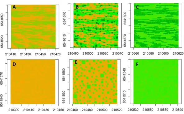
Figure 2 Spatial maps of neutral models.Spatial maps of neutral models used to simulate vegetation biomass for the following conditions: (A) Unfenced, unfertilized, (B) Unfenced, heterogeneously ized, (C) Unfenced-homogeneously fertilized, (D) Fenced, unfertilized, (E) Fenced, heterogeneously fertil-ized, (F) Fenced, homogeneously fertilized.
the mean of the biomass from the fenced, unfertilized experimental plot), (Fig. 2B) fenced-heterogeneous (biomass ofFig. 2Awas doubled for selected subplots, following the same subplot structure that was used in the field experiments), (Fig. 2C) fenced-homogenous (biomass ofFig. 2Awas doubled at every grid cell to mimic an evenly distributed fertilization response), (Fig. 2D) unfenced-unfertilized (biomass ofFig. 2Awas increased by 50% in response to a combined effect of biomass loss by grazing and biomass gain by manure nutrient additions by herbivores; the increase occurred at a subset of sites to mimic random movement patterns of herbivores), (Fig. 2E) unfenced-heterogeneous (biomass equaled biomass of herbivory only, fertilizer only, or herbivory+fertilizer), and (Fig. 2F) unfenced-homogenous (biomass of Fig. 2Dwas doubled at all grid cells to mimic the additive effects of herbivores and homogenous fertilizer additions).
The spatial structure of simulated landscapes was analyzed using the same maximum likelihood approach as described for empirical models and data was not transformed. The mean (µ) was estimated using a constant trend estimate. Given that the magnitude of observed and simulated biomass can change the amount of spatial variance, we scaled the nugget and sill parameters by dividing these parameters by the maximum calculated spatial autocorrelation in the data according to the ‘modulus’ method (Cressie, 1993).
RESULTS
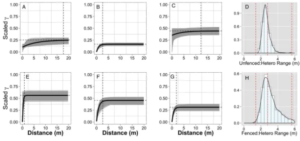
Figure 3 Empirical semivariograms.Empirical semi-variograms of vegetation biomass for each plot: (A) Unfenced, unfertilized, (B) Unfenced, Heterogeneously Fertilized, (C) Unfenced, homogeneously tilized, (E) Fenced, unfertilized, (F) Fenced, heterogeneously fertilized, (G) Fenced, homogeneously fer-tilized. Shaded lines represent semi-variogram models fitted during the bootstrapping procedure. Dashed vertical line represents the range value. Also shown: the sampling distribution of the range parameter for heterogeneously fertilized plots that were either (D) Unfenced, or (H) Fenced. The distribution was calcu-lated with a bootstrapping approach with maximum likelihood optimization. Dashed vertical lines repre-sent the hypotenuses of the 1×1 m (1.4), 2×2 (2.8), and 4×4 (5.7) sub-plots.
averaged 0.60±0.01% in unfertilized plots, 0.72 ±0.02% in heterogeneously fertilized plots, and 0.77±0.02% in homogenously fertilized plots, an increase of 20 % and 28%, respectively. Vegetation P concentration averaged 0.037±0.001 mg g−1in unfertilized plots, 0.056±0.002 mg g−1in heterogeneously fertilized, and 0.057±0.002 mg g−1in homogeneously fertilized plots, an increase of 34 and 35%, respectively. The vegetation N:P ratios ranged from a high of 17.9 in the fenced-unfertilized plot to 12.1 in the unfenced-homogenously fertilized plot. Vegetation C content averaged 44.6 ±0.13% across all six plots. Soil P and N were also higher following fertilization in the fenced plots, where these variables were measured (Table S1). Soil C ranged from 2.49±0.01% to 2.55 ±0.01% across plots. Soil pH was 4.27 in the unfertilized plot and 4.08 in fertilized plots. Confirming reference conditions, pH measured in a single control plot in 2011 prior to fertilization was 4.21±0.01.
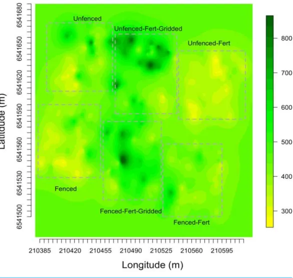
Figure 4 Kriged biomass map.Kriged map of biomass using ordinary kriging with a spatial covariance model optimized by a maximum likelihood analysis: (A) Unfenced, unfertilized, (B) Unfenced, heteroge-neously fertilized, (C) Unfenced, homogeheteroge-neously fertilized, (D) Fenced, unfertilized, (E) Fenced, hetero-geneously fertilized, (F) Fenced, homohetero-geneously fertilized.
biomass in fertilized subplots relative to areas outside of subplots or relative to other plots. These hotspots contributed to the higher than average biomass values for heterogeneously fertilized plots as a whole.
Normalized nugget/sill ratios represent the ratio of noise-to-structure in the semivariogram model, and thereby provide an estimate of the degree to which the overall variation in the model is spatially random. Nugget/sill ratios were highest in the unfenced, homogeneously fertilized plot (3.89), suggesting more random variation in the overall model variance, whereas ratios were lower (0–0.02) for heterogeneously fertilized or fenced treatments, suggesting that there was little contribution of spatially random processes in the overall model. These results support the expectation of strong spatial structure of biomass in response to nutrient addition, especially at the 2 meter scale.
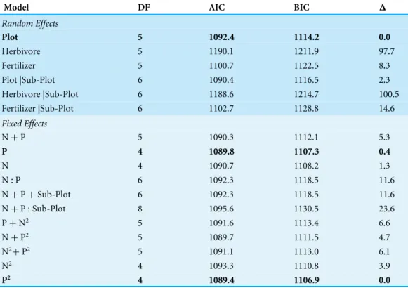
Table 2 Mixed model results comparing biomass to foliar nutrients.Results of the mixed model relat-ing biomass to foliar nutrients, where herbivory, fertilizer type, plot treatment, and subplot size were all tested as random effects; foliar N and P represented fixed effects upon biomass, and model error was as-sumed to be Gaussian. A normal likelihood function was minimized to estimate optimal regression coef-ficients for each mixed model formulation. Both Akaike’s Information Criterion (AIC) and Bayesian In-formation criterion (BIC) were used to compare different models. Delta (△) represents differences in BIC between the current model and the model with the lowest BIC.
Model DF AIC BIC 1
Random Effects
Plot 5 1092.4 1114.2 0.0
Herbivore 5 1190.1 1211.9 97.7
Fertilizer 5 1100.7 1122.5 8.3
Plot |Sub-Plot 6 1090.4 1116.5 2.3
Herbivore |Sub-Plot 6 1188.6 1214.7 100.5
Fertilizer |Sub-Plot 6 1102.7 1128.8 14.6
Fixed Effects
N+P 5 1090.3 1112.1 5.3
P 4 1089.8 1107.3 0.4
N 4 1090.7 1108.2 1.3
N : P 6 1092.3 1118.5 11.6
N+P+Sub-Plot 6 1092.3 1118.5 11.6
N+P : Sub-Plot 8 1095.6 1130.5 23.6
P+N2 5 1091.6 1113.4 6.6
N+P2 5 1089.7 1111.5 4.7
N2+P2 5 1091.1 1113.0 6.1
N2 4 1093.3 1110.8 3.9
P2 4 1089.4 1106.9 0.0
heterogeneously fertilized plot, where herbivores were absent. However, higher or lower range values were found for the other plots. Similar to results for biomass, the nugget:sill ratio in semivariogram models of vegetation % N and % P was highest in the unfertilized plots, suggesting a larger degree of spatially random processes contributing to overall variance. In turn, this indicates higher spatial structure captured in models of the fertilized treatments, relative to random processes. Semivariogram parameters of soil carbon and nutrients showed few differences among treatments where these were measured (fenced plots, only) (Table S3).
Mixed models used to predict biomass levels from N or P foliar concentrations, while treating plot and treatment as random effects, showed that biomass was best predicted by levels of foliar P, relative to foliar N alone or foliar N +P (Objective 2;Table 2). Although foliar P alone did better than foliar N alone as a fixed effect, the difference was marginal (<2 BIC). The ‘best’ model used only plot treatment type as a random effect, which outperformed model formulations using herbivory or fertilizer type and those with nested structures incorporating subplot size as random effects.
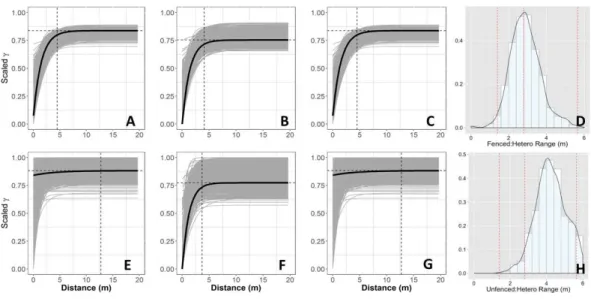
Figure 5 Semivariograms from neutral models.Simulated semivariograms of vegetation biomass for each plot from neutral landscape models: (A) Unfenced, unfertilized, (B) Unfenced, heterogeneously fer-tilized, (C) Unfenced, homogeneously ferfer-tilized, (D) Fenced, unferfer-tilized, (E) Fenced, heterogeneously fertilized, (F) Fenced, homogeneously fertilized. Shaded lines represent semi-variogram models fitted dur-ing the bootstrappdur-ing procedure. Dashed vertical line represents the optimal range value. Also shown: the sampling distribution of the range parameter for heterogeneously fertilized plots that were either (D) Un-fenced, or (H) Fenced. The distribution was calculated with a bootstrapping approach with maximum likelihood optimization.
(Objective 3;Fig. 5). Interestingly, the neutral models estimated higher range values (longer length scales) in fenced plots compared to unfenced plots, whereas empirical semivariogram models estimated longer length scales in unfenced plots.
DISCUSSION
Inferring the scale of grass response to nutrient additions
This study provided an opportunity to experimentally test the scale at which nutrient limitation is most strongly expressed, providing an alternative to studies in which spatial autocorrelation is observed post-hoc. Detecting the autocorrelation structure of an ecological pattern is a critical but insufficient approach for inferring an ecological process. A preferred approach, such as tested here, is to impose a pattern at a certain (set of) scale(s) and determine if that process responds at that scale(s). The benefit to this approach is a closer union between observed responses (biomass) and ecological processes (nutrient limitation) and the ability to compare responses across scales. Our results indicate that biomass responded to nutrient additions at all subplot scales, with spatial autocorrelation of the biomass response highest at the 2 ×2 m scale. Studies have found finer-grain spatial structure in grassland soil properties (Jackson & Caldwell, 1993a;Rietkerk et al., 2000;Augustine & Frank, 2001) while others have observed biomass responses to nutrient additions or herbivory at finer (Klaus et al., 2016) or broader (Lavado, Sierra & Hashimoto, 1995;Augustine & Frank, 2001;Pellegrini, 2016) scales, or a limited effect of scale altogether (Van der Waal et al., 2016) Indeed, we observed high nugget variance for soil nutrients and carbon under heterogeneous fertilization, implying variation below the scale of sampling. The response of biomass at the 2×2 m scale may thus reflect spatial patterns in species composition or plant groupings rather than soil characteristics, suggesting a possible influence of competitive exclusion, at least in fenced plots where soil nutrients were sampled.
Although vegetation responses were stronger at the 2×2 m grain, all subplots in the heterogeneous plots responded to nutrient additions, as observed in the kriged maps. As a result, the heterogeneous plots had greater average biomass than plots which were fertilized homogeneously, despite the fact that fertilizer was added equally on a per area basis for both treatments. Several other studies have found higher biomass following heterogeneous nutrient applications. For example, Day, Hutchings & John (2003) observed that heterogeneous spatial patterns of nutrient supply in early stages of grassland development led to enhanced nutrient acquisition and biomass productivity. Similarly,Du et al. (2012) observed increased plant biomass following heterogeneous nutrient fertilization in old-field communities in China. Mechanisms for enhanced productivity following heterogeneous nutrient supply are not clear but may include shifts in root structure and function or shifts in species dominance, which were not analyzed here. For example, roots may respond to patchiness in nutrient availability by modifying root lifespan, rooting structures, or uptake rate to maximize nutrient supply (Robinson, 1994;
Hodge, 2004). In turn, initial advantages afforded by plants in nutrient-rich locations may result in larger plants and advantages against competitive species, potentially via enhanced root growth (Casper, Cahill & Jackson, 2000).
Implications for understanding nutrient limitations
and P limitation in grasslands (Craine & Jackson, 2010), including the subtropics (Klaus et al., 2016).Ostertag (2010)also showed that there was a preference for P uptake in a nutrient limited ecosystem in Hawaii and suggested that foliar P accumulation may be a strategy to cope with variability in P availability. We found that P was the variable that explained most of the variation in the level of biomass response across all plots, followed by N. In addition, we saw a strong difference in N:P ratios between reference and fertilized plots. Many studies have used stoichiometric relationships of N and P to infer nutrient limitation (Koerselman & Meuleman, 1996;Reich & Oleksyn, 2004), although there are limits to this approach (Townsend et al., 2007;Ostertag, 2010). Using this index, our N:P ratios of vegetation in reference plots would indicate co-limitation for N and P prior to fertilization (N:P > 16). Addition of dual fertilizer appeared to alleviate P limitation more than N, with N:P ratios reduced one year following treatment, indicating N limitation or co-limitation with another element (N:P < 14). Grazing may also preferentially increase grass P concentrations in semi-arid systems in South Africa (Mbatha & Ward, 2010) and thus the cumulative impacts of preferential plant P uptake and P additions from manure may explain the high spatial structure observed in our grazed and fertilized plots.
Relating biomass response to nutrient limitation usingin situdata is complicated by processes such as luxury consumption (Ostertag, 2010), initial spatial patterns in soil fertility (Castrignano et al., 2000), root distribution, signaling and allocation (Aiken & Smucker, 1996), species and functional group shifts (Reich et al., 2003;Ratnam et al., 2008), or species’ differences in uptake rates or resorption (Townsend et al., 2007;Reed et al., 2012). Spatial patterns of finer-scale processes such as microbial community composition have also been explored and are known to influence rates of nutrient cycling (Ritz et al., 2004;
Smithwick et al., 2005). In the case of heterogeneous nutrient supply, species competitive relationships across space may be enhanced (Du et al., 2012) and may result in increases in plant diversity (Fitter, 1982;Wijesinghe, John & Hutchings, 2005), although other studies have found little evidence to support this claim (Gundale et al., 2011). Together, these factors may explain any unexplained variance of vegetation N and P concentrations that we observed. Shifts in species composition were likely minimal in this study given the short-term nature of the study (one year), but patchiness in biomass responses indicate size differences that could have modified competitive relationships in the future (Grime, 1973). Unfortunately, the site burned one year following the experiment, precluding additional tests of these relationships.
Herbivory-nutrient interactions
additions (Milchunas & Lauenroth, 1993;Adler, Raff & Lauenroth, 2001;Van der Waal et al., 2016). Interestingly, our empirical semivariogram model indicates longer range scales where herbivores were present compared to simulated semivariogram models, which may reflect homogenization of biomass through grazing and thus a greater top-down approach of herbivory on ecosystem productivity than previously appreciated (Van der Waal et al., 2016), or other complex interactions between grazing and fertilization not accounted for in the current study.
Uncertainties
There are several key uncertainties and caveats in applying our methodological approach more broadly. First, the experimental design described herein was labor-intensive, requiring both precision mapping of locations for nutrient additions and post-treatment vegetation sampling, as well as extensive replication of treatments that would respond to broader ecological patterns, i.e., grazing. This necessitated a trade-off between sampling effort across scales (subplots, plots). Important processes at scales above and below the extent and grain of sampling used here were likely important but were not included. Second, our neutral models assumed additive effects of herbivore activity and fertilization; in contrast, empirical results likely reflect complex, potentially non-additive, interactions between grazing and fertilization. Third, recent work has suggested that both nutrient patchiness and the form of nutrient limitation (e.g., N vs. P) may change seasonally (Klaus et al., 2016), which was not assessed here. Moreover, annual variation in precipitation, in our case a dry year followed by a wet year, may have influenced the level of biomass response to nutrient additions.
CONCLUSIONS
Understanding the factors that regulate ecosystem productivity, and the scales at which they operate, is critical for guiding ecosystem management activities aimed at maintaining landscape sustainability. New approaches are needed to characterize how ecosystems are spatially structured and to determine whether there are specific scale or scales of response that are most relevant. In South Africa, grasslands cover nearly one-third of the country and maintain the second-highest levels of biodiversity but are expected to undergo significant losses in biodiversity in coming decades due to increasing pressure from agricultural development and direct changes in climate (Biggs et al., 2008;Huntley & Barnard, 2012). We employed a neutral model approach to test for ecological process, an approach that has been advocated for decades (Turner, 1989) but which is rarely imposed (but seeWith, 1997;
ACKNOWLEDGEMENTS
We are deeply grateful to the support of Jan Venter, the Eastern Cape Parks and Tourism Board, and especially the Mkambathi Nature Reserve for allowing the establishment of the ‘‘Little Pennsylvania’’ study area. We are grateful to the hard work of the Parks and People 2010, 2011, and 2012 research teams, which included undergraduate students from The Pennsylvania State University who helped in all aspects of field research. Special thanks to the dedication of Sarah Hanson, Warren Reed, Shane Bulick, and Evan Griffin who assisted tirelessly with both field and laboratory work. We also thank the reviewers and editors for their insightful comments.
ADDITIONAL INFORMATION AND DECLARATIONS
Funding
This research was made possible through support from the National Science Foundation-Division of Environmental Biology grant (NSF-DEB 1045935) and a National Science Foundation-Research Experience for Undergraduates grant (NSF-DEB 1045935) to EAH Smithwick, and the Penn State College of Earth and Mineral Sciences George H. Deike, Jr. Research Grant. The funders had no role in study design, data collection and analysis, decision to publish, or preparation of the manuscript.
Grant Disclosures
The following grant information was disclosed by the authors:
National Science Foundation-Division of Environmental Biology: NSF-DEB 1045935. National Science Foundation-Research Experience for Undergraduates: NSF-DEB 1045935. Penn State College of Earth and Mineral Sciences George H. Deike, Jr. Research Grant.
Competing Interests
The authors declare there are no competing interests.
Author Contributions
• Erica A.H. Smithwick conceived and designed the experiments, performed the experiments, analyzed the data, wrote the paper, prepared figures and/or tables. • Douglas C. Baldwin performed the experiments, analyzed the data, prepared figures
and/or tables, reviewed drafts of the paper.
• Kusum J. Naithani analyzed the data, prepared figures and/or tables, reviewed drafts of the paper.
Field Study Permissions
The following information was supplied relating to field study approvals (i.e., approving body and any reference numbers):
South Africa Eastern Cape Parks and Tourism Agency, Permit #RA0081.
Data Availability
The following information was supplied regarding data availability: The raw data has been supplied as aSupplemental Dataset.
Supplemental Information
Supplemental information for this article can be found online athttp://dx.doi.org/10.7717/ peerj.2745#supplemental-information.
REFERENCES
Adler PB, Raff DA, Lauenroth WK. 2001.The effect of grazing on the spatial heterogene-ity of vegetation.Oecologia128:465–479DOI 10.1007/s004420100737.
Aiken RM, Smucker AJM. 1996.Root system regulation of whole plant growth.Annual Review of Phytopathology34:325–346DOI 10.1146/annurev.phyto.34.1.325. Auerswald K, Mayer F, Schnyder H. 2010.Coupling of spatial and temporal pattern of
cattle excreta patches on a low intensity pasture.Nutrient Cycling in Agroecosystems
88:275–288DOI 10.1007/s10705-009-9321-4.
Augustine DJ, Frank DA. 2001.Effects of migratory grazers on spatial heterogene-ity of soil nitrogen properties in a grassland ecosystem.Ecology82:3149–3162 DOI 10.1890/0012-9658(2001)082[3149:EOMGOS]2.0.CO;2.
Augustine DJ, McNaughton SJ, Frank DA. 2003.Feedbacks between soil nutrients and large herbivores in a managed savanna ecosystem.Ecological Applications
13:1325–1337DOI 10.1890/02-5283.
Beale CM, Lennon JJ, Yearsley JM, Brewer MJ, Elston DA. 2010.Regression analysis of spatial data.Ecology Letters13:246–264DOI 10.1111/j.1461-0248.2009.01422.x. Ben Wu X, Archer SR. 2005.Scale-dependent influence of topography-based hydrologic
features on patterns of woody plant encroachment in savanna landscapes.Landscape
Ecology 20:733–742DOI 10.1007/s10980-005-0996-x.
Biggs R, Simons H, Bakkenes M, Scholes RJ, Eickhout B, Van Vuuren D, Alkemade R. 2008.Scenarios of biodiversity loss in southern Africa in the 21st century.Global
Environmental Change18:296–309DOI 10.1016/j.gloenvcha.2008.02.001.
Box GEP, Cox DR. 1964.An analysis of transformations.Journal of the Royal Statistical Society Series B-Statistical Methodology 26:211–252.
Bransby D, Tainton N. 1977.The disc pasture meter: possible applications in grazing management.Proclamations of the Grassland Society of South Africa12:115–118 DOI 10.1080/00725560.1977.9648818.
Burnham KP, Anderson DR. 2002.Model selection and multimodel inference: a practical information-theoretic approach. New York: Springer-Verlag.
Casper BB, Cahill JF, Jackson RB. 2000. Plant competition in spatially heterogeneous environments. In: Hutchings MJ, John EA, Stewart AJA, eds.Ecological consequences of environmental heterogeneity. Oxford: Blackwell Science, 111–130.
CEPF. 2010.Maputaland-pondoland-albany ecosystem profile summary. Arlington: Conservation International.
Craine JM, Jackson RD. 2010.Plant nitrogen and phosphorus limitation in 98 North American grassland soils.Plant and Soil334:73–84DOI 10.1007/s11104-009-0237-1. Craine JM, Morrow C, Stock WD. 2008.Nutrient concentration ratios and co-limitation
in South African grasslands.New Phytologist179:829–836 DOI 10.1111/j.1469-8137.2008.02513.x.
Cressie N. 1988.Spatial prediction and ordinary kriging.Mathematical Geology
20:405–421DOI 10.1007/BF00892986.
Cressie N. 1993.Statistics for spatial data. New York: John Wiley & Sons, Inc.
Day KJ, Hutchings MJ, John EA. 2003.The effects of spatial pattern of nutrient supply on the early stages of growth in plant populations.Journal of Ecology 91:305–315 DOI 10.1046/j.1365-2745.2003.00763.x.
Diggle PJ, Ribeiro Jr PJ, Christensen OF. 2003. An introduction to model-based
geostatistics. In: Möller J, ed.Spatial statistics and computational methods. New York: Springer, 43–86.
Dijkstra F, Wrage K, Hobbie S, Reich P. 2006.Tree patches show greater N losses but maintain higher soil N availability than grassland patches in a frequently burned oak savanna.Ecosystems9:441–452DOI 10.1007/s10021-006-0004-6.
Domingues TF, Meir P, Feldpausch TR, Saiz G, Veenendaal EM, Schrodt F, Bird M, Djagbletey G, Hien F, Compaore H, Diallo A, Grace J, Lloyd J. 2010.Co-limitation of photosynthetic capacity by nitrogen and phosphorus in West Africa woodlands.
Plant Cell and Environment 33:959–980DOI 10.1111/j.1365-3040.2010.02119.x. Du F, Xu XX, Zhang XC, Shao MG, Hu LJ, Shan L. 2012.Responses of old-field
vegetation to spatially homogenous or heterogeneous fertilisation: implications for resources utilization and restoration.Polish Journal of Ecology60:133–144.
Dungan JL, Perry JN, Dale MRT, Legendre P, Citron-Pousty S, Fortin MJ, Jakomulska A, Miriti M, Rosenberg MS. 2002.A balanced view of scale in spatial statistical analysis.Ecography25:626–640DOI 10.1034/j.1600-0587.2002.250510.x. Eckert D, Sims JT. 1995. Recommended soil pH and lime requirement tests. In:
Agricultural experiment station. Newark: University of Delaware.
Ettema CH, Wardle DA. 2002.Spatial soil ecology.Trends in Ecology & Evolution
17:177–183DOI 10.1016/S0169-5347(02)02496-5.
Fajardo A, McIntire EJB. 2007.Distinguishing microsite and competition processes in tree growth dynamics: an a priori spatial modeling approach.American Naturalist
169:647–661DOI 10.1086/513492.
Fitter AH. 1982.Influence of soil heterogeneity on the coexistence of grassland species.
Journal of Ecology70:139–148 DOI 10.2307/2259869.
Fu WJ, Zhao KL, Jiang PK, Ye ZQ, Tunney H, Zhang CS. 2013.Field-scale variability of soil test phosphorus and other nutrients in grasslands under long-term agricultural managements.Soil Research51:503–512DOI 10.1071/SR13027.
Fuhlendorf SD, Smeins FE. 1999.Scaling effects of grazing in a semi-arid grassland.
Journal of Vegetation Science10:731–738DOI 10.2307/3237088.
Gil MA, Jiao J, Osenberg CW. 2016.Enrichment scale determines herbivore control of primary producers.Oecologia180:833–840DOI 10.1007/s00442-015-3505-1. Grime JP. 1973.Competitive exclusion in herbaceous vegetation.Nature 242:344–347
DOI 10.1038/242344a0.
Gundale MJ, Fajardo A, Lucas RW, Nilsson M-C, Wardle DA. 2011.Resource hetero-geneity does not explain the diversity-productivity relationship across a boreal island fertility gradient.Ecography34:887–896DOI 10.1111/j.1600-0587.2011.06853.x. Hedin LO. 2004.Global organization of terrestrial plant-nutrient interactions.
Proceedings of the National Academy of Sciences of the United States of America
101:10849–10850DOI 10.1073/pnas.0404222101.
Hibbard KA, Archer S, Schimel DS, Valentine DW. 2001.Biogeochemical changes accompanying woody plant encroachment in a subtropical savanna.Ecology
82:1999–2011DOI 10.1890/0012-9658(2001)082[1999:BCAWPE]2.0.CO;2. Hodge A. 2004.The plastic plant: root responses to heterogeneous supplies of nutrients.
New Phytologist 162:9–24DOI 10.1111/j.1469-8137.2004.01015.x.
Horn S, Hempel S, Ristow M, Rillig MC, Kowarik I, Caruso T. 2015.Plant com-munity assembly at small scales: spatial vs. environmental factors in a Euro-pean grassland.Acta Oecologica-International Journal of Ecology 63:56–62 DOI 10.1016/j.actao.2015.01.004.
Horneck DA, Miller RO. 1998. Determination of total nitrogen in plant tissue. In: Kalra YP, ed.Handbook and reference methods for plant analysis. New York: CRC Press. House JI, Archer S, Breshears DD, Scholes RJ. 2003.Conundrums in mixed
woody-herbaceous plant systems.Journal of Biogeography30:1763–1777 DOI 10.1046/j.1365-2699.2003.00873.x.
Huang C-YL, Schulte EE. 1985.Digestion of plant tissue for analysis by ICP emission spectroscopy.Communications in Soil Science and Plant Analysis16:943–958 DOI 10.1080/00103628509367657.
Huntley B, Barnard P. 2012.Potential impacts of climatic change on southern African birds of fynbos and grassland biodiversity hotspots.Diversity and Distributions
18:769–781DOI 10.1111/j.1472-4642.2012.00890.x.
Jackson RB, Caldwell MM. 1993a.Geostatistical patterns of soil heterogeneity around individual perennial plants.Journal of Ecology81:683–692DOI 10.2307/2261666. Jackson RB, Caldwell MM. 1993b.The scale of nutrient heterogeneity around
Jean PO, Bradley RL, Tremblay JP, Cote SD. 2015.Combining near infrared spectra of feces and geostatistics to generate forage nutritional quality maps across landscapes.
Ecological Applications25:1630–1639DOI 10.1890/14-1347.1.
Jenerette GD, Wu J. 2004.Interactions of ecosystem processes with spatial heterogeneity in the puzzle of nitrogen limitation.Oikos107:273–282
DOI 10.1111/j.0030-1299.2004.13325.x.
Kerley GIH, Knight MH, DeKock M. 1995.Desertification of subtropical thicket in the Eastern Cape, South Africa: are there alternatives?Environmental Monitoring and
Assessment 37(1):211–230DOI 10.1007/BF00546890.
Klaus VH, Boch S, Boeddinghaus RS, Holzel N, Kandeler E, Marhan S, Oelmann Y, Prati D, Regan KM, Schmitt B, Sorkau E, Kleinebecker T. 2016.Temporal and small-scale spatial variation in grassland productivity, biomass quality, and nutrient limitation.Plant Ecology 217:843–856DOI 10.1007/s11258-016-0607-8.
Koerselman W, Meuleman AFM. 1996.The vegetation N:P ratio: a new tool to de-tect the nature of nutrient limitation.Journal of Applied Ecology33:1441–1450 DOI 10.2307/2404783.
Lambers H, Raven JA, Shaver GR, Smith SE. 2008.Plant nutrient-acquisition strategies change with soil age.Trends in Ecology & Evolution23:95–103 DOI 10.1016/j.tree.2007.10.008.
Lavado RS, Sierra JO, Hashimoto PN. 1995.Impact of grazing on soil nutrients in a pampean grassland.Journal of Range Management49:452–457.
LeBauer DS, Treseder KK. 2008.Nitrogen limitation of net primary produc-tivity in terrestrial ecosystems is globally distributed.Ecology 89:371–379 DOI 10.1890/06-2057.1.
Lechmere-Oertel RG, Cowling RM, Kerley GIH. 2005.Landscape dysfunction and reduced spatial heterogeneity in soil resources and fertility in semi-arid succulent thicket, South Africa.Austral Ecology30:615–624
DOI 10.1111/j.1442-9993.2005.01495.x.
Levin SA. 1992.The problem of pattern and scale in ecology.Ecology73:1943–1967 DOI 10.2307/1941447.
Liski J. 1995.Variation in soil organic carbon and thickness of soil horizons within a boreal forest stand—effects of trees and implications for sampling.Silva Fennica
29:255–266DOI 10.14214/sf.a9212.
Liu C, Song XX, Wang L, Wang DL, Zhou XM, Liu J, Zhao X, Li J, Lin HJ. 2016. Effects of grazing on soil nitrogen spatial heterogeneity depend on herbivore assemblage and pre-grazing plant diversity.Journal of Applied Ecology53:242–250 DOI 10.1111/1365-2664.12537.
Mbatha KR, Ward D. 2010.The effects of grazing, fire, nitrogen and water availability on nutritional quality of grass in semi-arid savanna, South Africa.Journal of Arid Environments74:1294–1301DOI 10.1016/j.jaridenv.2010.06.004.
Milchunas DG, Lauenroth WK. 1993.Quantitative effects of grazing on vegetation and soils over a global range of environments.Ecological Monographs63:327–366 DOI 10.2307/2937150.
Millar RB, Anderson MJ. 2004.Remedies for pseudoreplication.Fisheries Research
70:397–407DOI 10.1016/j.fishres.2004.08.016.
Miller J, Franklin J, Aspinall R. 2007.Incorporating spatial dependence in predictive vegetation models.Ecological Modelling 202:225–242
DOI 10.1016/j.ecolmodel.2006.12.012.
Mills AJ, Rogers KH, Stalmans M, Witkowski ETF. 2006.A framework for exploring the determinants of savanna and grassland distribution.Bioscience56:579–589 DOI 10.1641/0006-3568(2006)56[579:AFFETD]2.0.CO;2.
Ngatia LW, Turner BL, Njoka JT, Young TP, Reddy KR. 2015.The effects of herbivory and nutrients on plant biomass and carbon storage in Vertisols of an East African savanna.Agriculture Ecosystems & Environment 208:55–63 DOI 10.1016/j.agee.2015.04.025.
Okin GS, Mladenov N, Wang L, Cassel D, Caylor KK, Ringrose S, Macko SA. 2008. Spatial patterns of soil nutrients in two southern African savannas.Journal of
Geophysical Research-Biogeosciences113:2156–2202DOI 10.1029/2007JG000584.
Ostertag R. 2010.Foliar nitrogen and phosphorus accumulation responses after fertiliza-tion: an example from nutrient-limited Hawaiian forests.Plant and Soil334:85–98 DOI 10.1007/s11104-010-0281-x.
Pellegrini AFA. 2016.Nutrient limitation in tropical savannas across multiple scales and mechanisms.Ecology 97:313–324.
Pennanen T, Liski J, Kitunen V, Uotila J, Westman CJ, Fritze H. 1999.Structure of the microbial communities in coniferous forest soils in relation to site fertility and stand development stage.Microbial Ecology38:168–179 DOI 10.1007/s002489900161. Pickett STA, Cadenasso ML, Benning TL. 2003. Biotic and abiotic variability as key determinants of savanna heterogeneity at multiple spatiotemporal scales. In: Du Toit SR, Rogers KH, Biggs HC, eds.The kruger experience: ecology and management of savanna heterogeneity. Washington, D.C.: Island Press, 22–40.
R Development Core Team. 2014.R: a language and environment for statistical computing. Vienna: R Foundation for Statistical Computing.Available athttp: // www.R-project.org.
Ratnam J, Sankaran M, Hanan NP, Grant RC, Zambatis N. 2008.Nutrient resorption patterns of plant functional groups in a tropical savanna: variation and functional significance.Oecologia157:141–151DOI 10.1007/s00442-008-1047-5.
Reed SC, Townsend AR, Davidson EA, Cleveland CC. 2012.Stoichiometric patterns in foliar nutrient resorption across multiple scales.New Phytologist 196:173–180 DOI 10.1111/j.1469-8137.2012.04249.x.
Reich PB, Buschena C, Tjoelker MG, Wrage K, Knops J, Tilman D, Machado JL. 2003. Variation in growth rate and ecophysiology among 34 grassland and savanna species under contrasting N supply: a test of functional group differences.New Phytologist
Reich PB, Oleksyn J. 2004.Global patterns of plant leaf N and P in relation to tempera-ture and latitude.Proceedings of the National Academy of Sciences of the United States
of America101:11001–11006DOI 10.1073/pnas.0403588101.
Remsburg AJ, Turner MG. 2006.Amount, position, and age of coarse wood influence litter decomposition in postfirePinus contortastands.Canadian Journal Forest
Research36:2112–2123DOI 10.1139/x06-079.
Ribeiro Jr PJ, Diggle PJ. 2001.geoR: a package for geostatistical analysis.R News1:14–18. Rietkerk M, Ketner P, Burger J, Hoorens B, Olff H. 2000.Multiscale soil and vegetation
patchiness along a gradient of herbivore impact in a semi-arid grazing system in West Africa.Plant Ecology148:207–224DOI 10.1023/A:1009828432690. Ritz K, McNicol W, Nunan N, Grayston S, Millard P, Atkinson D, Gollotte A,
Habeshaw D, Boag B, Clegg CD, Griffiths BS, Wheatley RE, Glover LA, Mc-Caig AE, Prosser JI. 2004.Spatial structure in soil chemical and microbiologi-cal properties in an upland grassland.FEMS Microbiology Ecology49:191–205 DOI 10.1016/j.femsec.2004.03.005.
Robertson GP, Crum JR, Ellis BG. 1993.The spatial variability of soil resources following long-term disturbance.Oecologia96:451–456DOI 10.1007/BF00320501.
Robinson D. 1994.The response of plants to nonuniform supplies of nutrients.New Phytologist 127:635–674DOI 10.1111/j.1469-8137.1994.tb02969.x.
Rogers KH. 2003. Adopting a heterogeneity paradigm: implications for management of protected savannas. In: Du Toit SR, Rogers KH, Biggs HC, eds.The kruger experience: ecology and management of savanna heterogeneity. Washington, D.C.: Island Press, 41–58.
Sandel B. 2015.Towards a taxonomy of spatial scale-dependence.Ecography38:358–369 DOI 10.1111/ecog.01034.
Schoennagel T, Smithwick EAH, Turner MG. 2008.Landscape heterogeneity following large fires: insights from Yellowstone National Park, USA.International Journal of
Wildland Fire17:742–753DOI 10.1071/WF07146.
Schoolmaster DR, Mittelbach GG, Gross KL. 2014.Resource competition and commu-nity response to fertilization: the outcome depends on spatial strategies.Theoretical
Ecology 7:127–135DOI 10.1007/s12080-013-0205-5.
Senft RL, Coughenour MB, Bailey DW, Rittenhouse LR, Sala OE, Swift DM. 1987. Large herbivore foraging and ecological hierarchies.Bioscience37:789–797 DOI 10.2307/1310545.
Shackleton CM. 1990.Seasonal changes in biomass concentration in three coastal grassland communities in Transkei.Journal of Grassland Society of Southern Africa
7:265–269DOI 10.1080/02566702.1990.9648246.
Shackleton CM, Granger JE, McKenzie B, Mentis MT. 1991.Multivariate analysis of coastal grasslands at Mkambati Game Reserve, north-eastern Pondoland, Transkei.
Bothalia21:91–107.
Smithwick EAH, Harmon ME, Domingo JB. 2003.Modeling multiscale effects of light limitations and edge-induced mortality on carbon stores in forest landscapes.
Smithwick EAH, Mack MC, Turner MG, Chapin FS, Zhu J, Balser TC. 2005. Spa-tial heterogeneity and soil nitrogen dynamics in a burned black spruce for-est stand: distinct controls at different scales.Biogeochemistry76:517–537 DOI 10.1007/s10533-005-0031-y.
Smithwick EAH, Naithani KJ, Balser TC, Romme WH, Turner MG. 2012.Post-fire spatial patterns of soil nitrogen mineralization and microbial abundance.PLoS ONE
7:e50597DOI 10.1371/journal.pone.0050597.
Stohlgren TJ, Falkner MB, Schell LD. 1995.A modified-Whittaker nested vegetation sampling method.Vegetatio117:113–121DOI 10.1007/BF00045503.
Townsend AR, Cleveland CC, Asner GP, Bustamante MMC. 2007.Controls over foliar N : P ratios in tropical rain forests.Ecology 88:107–118
DOI 10.1890/0012-9658(2007)88[107:COFNRI]2.0.CO;2.
Turner MG. 1989.Landscape ecology: the effect of pattern on process.Annual Review of Ecology and Systematics20:171–197DOI 10.1146/annurev.es.20.110189.001131. Turner MG, Donato DC, Romme WH. 2013.Consequences of spatial heterogeneity
for ecosystem services in changing forest landscapes: priorities for future research.
Landscape Ecology28:1081–1097DOI 10.1007/s10980-012-9741-4.
Turner MG, Gardner RH. 2015.Landscape ecology in theory and practice: pattern and process. Second edition. New York: Springer.
Turner MG, Romme WH, Smithwick EAH, Tinker DB, Zhu J. 2011.Variation in aboveground cover influences soil nitrogen availability at fine spatial scales following severe fire in subalpine conifer forests.Ecosystems14:1081–1095 DOI 10.1007/s10021-011-9465-3.
Turner MG, Smithwick EAH, Metzger KL, Tinker DB, Romme WH. 2007.Inorganic nitrogen availability after severe stand-replacing fire in the Greater Yellowstone Ecosystem.Proceedings of the National Academy of Sciences of the United States of
America104:4782–4789DOI 10.1073/pnas.0700180104.
Van der Waal C, De Kroon H, Van Langevelde F, De Boer WF, Heitkönig IMA, Slotow R, Pretorius Y, Prins HHT. 2016.Scale-dependent bi-trophic interactions in a semi-arid savanna: how herbivores eliminate benefits of nutrient patchiness to plants.
Oecologia181:1173–1185DOI 10.1007/s00442-016-3627-0.
Veldhuis MP, Hulshof A, Fokkema W, Berg MP, Olff H. 2016.Understanding nutrient dynamics in an African savanna: local biotic interactions outweigh a major regional rainfall gradient.Journal of Ecology104:913–923DOI 10.1111/1365-2745.12569. Vitousek P, Howarth RW. 1991.Nitrogen limitation on land and in the sea: how can it
occur?Biogeochemistry 13:87–115.
Vitousek PM, Sanford RL. 1986.Nutrient cycing in moist tropical forests.Annual Review of Ecology and Systematics17:137–167DOI 10.1146/annurev.es.17.110186.001033. Wang LX, D’Odorico P, O’Halloran LR, Caylor K, Macko S. 2010.Combined effects
of soil moisture and nitrogen availability variations on grass productivity in African savannas.Plant and Soil328:95–108DOI 10.1007/s11104-009-0085-z.
Wijesinghe DK, John EA, Hutchings MJ. 2005.Does pattern of soil resource heterogene-ity determine plant communheterogene-ity structure? An experimental investigation.Journal of Ecology 93:99–112DOI 10.1111/j.0022-0477.2004.00934.x.
With KA. 1997.The application of neutral landscape models in conservation biology.
Conservation Biology11:1069–1080DOI 10.1046/j.1523-1739.1997.96210.x.
With KA, Crist TO. 1995.Critical thresholds in species responses to landscape structure.
Ecology 76:2446–2459DOI 10.2307/2265819.
Wolf AM, Beegle DB. 1995. Recommended soil testing procedures for the northeastern United States. In:Agricultural experiment station. Newark: University of Delaware. Xu C, He HS, Hu Y, Chang Y, Li X, Bu R. 2005.Latin hypercube sampling and