An Optimized Analogy-Based Project Effort
Estimation
Mohammad Azzeh
Faculty of Information Technology Applied Science UniversityAmman,Jordan POBOX 166
Yousef Elsheikh
Faculty of Information Technology Applied Science University
Amman, Jordan
Marwan Alseid
Faculty of Information Technology Applied Science University
Amman, Jordan
Abstract—Despite the predictive performance of Analogy-Based Estimation (ABE) in generating better effort estimates, there is no consensus on: (1) how to predetermine the appropriate number of analogies, (2) which adjustment technique produces better estimates. Yet, there is no prior works attempted to optimize both number of analogies and feature distance weights for each test project. Perhaps rather than using fixed number, it is better to optimize this value for each project individually and then adjust the retrieved analogies by optimizing and approximating complex relationships between features and reflects that approximation on the final estimate. The Artificial Bees Algorithm is utilized to find, for each test project, the appropriate number of closest projects and features distance weights that are used to adjust those analogies’ efforts. The proposed technique has been applied and validated to 8 publically datasets from PROMISE repository. Results obtained show that: (1) the predictive performance of ABE has noticeably been improved; (2) the number of analogies was remarkably variable for each test project. While there are many techniques to adjust ABE, Using optimization algorithm provides two solutions in one technique and appeared useful for datasets with complex structure.
Keywords—Cost Estimation; Effort Estimation by Analogy; Bees Optimization Algorithm
I. INTRODUCTION
Analogy-Based Estimation (ABE) has preserved popularity within software engineering research community because of its outstanding performance in prediction when different data types are used [1, 15]. The idea behind this method is rather simple such that the new project’s effort can be estimated by reusing efforts about similar, already documented projects in a dataset, where in a first step one has to identify similar projects which contain the useful predictions [15]. The predictive performance of ABE relies significantly on the choice of two interrelated parameters: number of nearest analogies and adjustment strategy [8]. The goal of using adjustment in ABE is twofold: (1) minimizing the difference between a new project and its nearest analogies, and (2) producing more successful estimates in comparison to original ABE [2]. If the researchers read the literature on ABE, they will encounter large number of ABE models that use variety of adjustment strategies. Those strategies suffer from common problems such as they are not able to produces stable results when applied in different contexts as well as they use fixed number of analogies for the whole dataset [1]. Using fixed number of analogies has been proven to be unsuccessful
in many situations because it depends heavily on expert opinion and requires extensive experimentation to identify the best k value, which might not be predictive for individual projects [2].
The aim of this work is therefore to propose a new method based on Artificial Bees Algorithm (BA) [14] to adjust ABE by optimizing the feature similarity coefficients that minimizes difference between new project and its nearest projects, and predicting the best k number of nearest analogies. The paper is structured as follows: Section 2 introduces an overview to ABE and adjustment methods. Section 3 presents the proposed adjustment method. Section 4 presents research methodology. Section 5 shows obtained results. Finally the paper ends with our conclusions.
II. RELATED WORKS
ABE method generates new prediction based on assumption that similar projects with respect to features description have similar efforts [8, 15]. Adjustment is a part of ABE that attempts to minimize the difference between new observation (eˆi) and each nearest similar observation (ei), then reflects that difference on the derived solution in order to obtain better solution ( et ). Consequentially, all adjusted solutions are aggregated using simple statistical methods such as mean ( et k
kiei1
1 ˆ ). In previous study [17] we investigated the performance of BA, on adjusting ABE and finding best k value for the whole dataset. This model showed some improvements on the accuracy, but on the other side it did not solve the problem of predicting the best k value for each individual project. In addition the solution space of BA was a challenge because there was only one common weight for all nearest analogies. The used optimization criterion (i.e. MMRE) was problematic because it was proven to be biased towards underestimation. For all these reason and since we need to compare our proposed model with validated and replicated models, we excluded this model from comparison later in this paper. This paper thereby attempts to solve abovementioned limitations.
Jorgenson et al. [6] proposed Regression Towards the Mean (RTM) to adjust projects based on their productivity values. Chiu and Huang [4] proposed another adjustment based on Genetic Algorithm (GA) to optimize the coefficient αj for each feature distance based on minimizing performance measure. Recently, Li et al. [10] proposed the use of Neural Network (NN) to learn the difference between projects and reflects the difference on the final estimate. Further details about these methods and their functions can be found in [1].
Indeed, the most important questions to consider when to use such methods is how to predict the best number of nearest analogies (k). In recent years various approaches have been proposed to specify this number such as: 1) fixed number selection (i.e. k=1, 2, 3…etc) as in studies of [7, 11, 12, 16], 2) Dynamic selection based on clustering as in study of [2, 17]. 3) Similarity threshold based selection as in studies of [5, 9]. Generally, these studies except [2] use the same k value for all projects in the dataset which does not necessarily produce best performance for each individual project. On the other hand, the certain problem with [2] is that it does not include adjustment method but it predicts the best k value based on the structure of dataset.
III. THE PROPOSED METHOD (OABE)
The proposed adjustment method starts with Bees Algorithm in order to find out, for each project: (1) the feature weights (w), and (2) the best k number of nearest analogies that minimize mean absolute error. The search space of BA can be seen as a set of n weight matrixes where the size of each matrix (i.e. solution) is k × m. That means each possible solution contains weight matrix with dimension equivalent to the number of analogies (k) and number of features (m) as shown in Figure 1. The number of rows (i.e. k) and weight values are initially generated by random. Each row represents weights for one selected analogy and accordingly
mj wj1 1. In each run the algorithm selects the top k nearest analogies based on the number of k weights in the search space. Then each selected analogy is adjusted with corresponding weights taken from the matrix w as shown Eq.1. The algorithm continues searching until the value of Mean Error (i.e.
k
j ij k
MR
1
1 ) between new project and its k analogies is minimized. The optimized k value and weight matrix are then applied to Eqs. 1, 2 and 3 to generate new estimate. The new integration between ABE with BA will be called Optimized Analogy Based Estimation (hereafter OABE).
km k
k
m m
w w
w
w w
w
w w
w w
2 1
2 22
21
1 12
11
Fig. 1. Weight Matrix for one solution in the search space
∑
mj wij ftj-fij mij 1 ( )
1
(1)
ij i e i
e
ˆ (2)
∑
ki i ki k ri ei
t e
1
1 1 ˆ
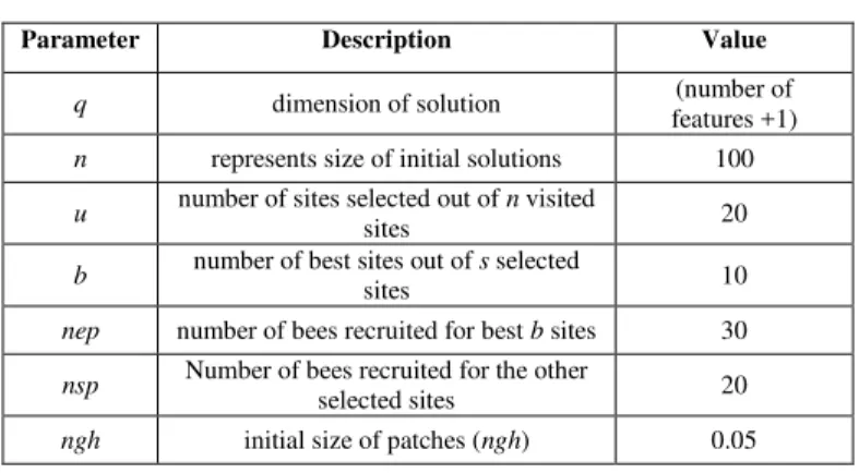
(3)The setting parameters for AB have been found after performing sensitivity analysis on the employed datasets to see the appropriate values. Table I shows BA parameters, their abbreviations and initial values used in this study. Below we briefly describe the process of BA in finding best k values and the corresponding weights for each new project. The algorithm starts with an initial set of weight matrixes generated after randomly initializing k for each matrix. The solutions are assessed and sorted in ascending order after they are being evaluated based on MR. The best from 1 to b solutions are being selected for neighborhood search for better solutions, and form new patch. Similarly, a number of bees (nsp) are also recruited for each solution ranked from b+1 to u, to search in the neighborhood. The best solution in each patch will replace the old best solution in that patch and the remaining bees will be replaced randomly with other solutions. The algorithm continues searching in the neighborhood of the selected sites, recruiting more bees to search near to the best sites which may have promising solutions. These steps are repeated until the criterion of stop (minimum MR) is met or the number of iteration has finished.
TABLE I. BA PARAMETERS
Parameter Description Value
q dimension of solution (number of
features +1) n represents size of initial solutions 100
u number of sites selected out of n visited
sites 20
b number of best sites out of s selected
sites 10
nep number of bees recruited for best b sites 30
nsp Number of bees recruited for the other selected sites 20
ngh initial size of patches (ngh) 0.05
IV. METHODOLOGY A. Datasets
TABLE II. DESCRIPTIVE STATISTICS OF THE DATASETS
Dataset Feature Size Effort Data
Min Max Mean Skew
Albrecht 7 24 1 105 22 2.2
Kemerer 7 15 23.2 1107.3 219.2 2.76
Nasa 3 18 5 138.3 49.47 0.57
Desharnais 12 77 546 23940 5046 2.0
COCOMO 17 63 6 11400 683 4.4
China 18 499 26 54620 3921 3.92 Maxwell 27 62 583 63694 8223.2 3.26 Telecom 3 18 23.54 1115.5 284.33 1.78
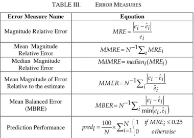
B. Performance measures
A key question to any estimation model is whether the predications are accurate, the difference between the actual effort (ei) and the predicted effort (eˆi) should be as small as possible because large deviation will have opposite effect on the development progress of the new software project [13]. This section describes several performance measures used in this research as shown in Table III. Although some measures such as MMRE, MMER have been criticized as biased to under and over estimations, we insist to use them because they are widely used in commenting on the success of predictions [13].
TABLE III. ERROR MEASURES
Error Measure Name Equation
Magnitude Relative Error
i e i e i e MRE ˆ
Mean Magnitude
Relative Error
iMREi
N
MMRE 1
Median Magnitude Relative Error
) (MREi i median MdMRE
Mean Magnitude of Error
Relative to the estimate
i ei i e i e N MMER ˆ ˆ 1
Mean Balanced Error
(MBRE)
i ei ei i e i e N MBER ˆ , min ˆ 1
Prediction Performance
N i otherwise i MRE if N l pred 1 0 25 . 0 1 100
Interpreting these error measures without any statistical test can lead to conclusion instability, therefore we used win-tie-loss algorithm [8] to compare the performance of OABE to other estimation methods. We first check if two methods methodi; methodj are statistically different according to the
Wilcoxon test. If so, we update wini; winj and lossi; lossjafter
checking which one is better according to the performance measure at hand; otherwise we increase tiei and tiej. The
performance measures used here are MRE, MMRE, MdMRE, MMER, MBER and Pred25. Algorithm 1 illustrates the
win-tie-loss algorithm [8]. Also, the Bonferroni-Dunn test is used to perform multiple comparisons for different models based on the absolute error to check whether there are differences in population rank means among more than populations.
Algorithm 1. Pseudocode of win-tie-loss algorithm betweenmethodi and
methodjbased on performance measure E [8]
1: Wini=0,tiei=0,lossi=0 2: Winj=0,tiej=0;lossj=0
3: if Wilcoxon (MRE(methodi), MRE(methodj), 95) says they are the same then
4: tiei = tiei + 1; 5: tiej = tiej + 1; 6:else
7: if better(E(methodi), E(methodj)) then 8: wini = wini + 1
9: lossj = lossj + 1 10: else
11: winj = winj + 1 12: lossi = lossi + 1 13:end if 14: end if
V. RESULTS
This section presents performance figures of OABE against various adjustment techniques used in constructing ABE models. Since the selection of the best k setting in OABE is dynamic, there was no need to pre-set the best k value. In contrast, for other variants of adjustment techniques there was necessarily finding the best k value that almost fits each model, therefore we applied different k settings from 1 to 5 on each model as suggested by Li et al. [9] and the setting that produces best overall performance has been selected for comparison with other different models. Tables IV, V, VI, VII and VIII summarize the resulting performance figures for all investigated ABE models. The most successful method should have lower MMRE, MdMRE, MMER, MBER and higher Pred25. The obtained results suggest that the OABE produced
accurate predictions than other methods with quite good performance figures over most datasets.
TABLE IV. MMRE RESULTS
Dataset OABE LSE MLFE RTM GA NN Albrecht 40.2 62.9 65.2 61.2 45.4 51.2 Kemerer 39.6 41.4 64.5 44.6 60.4 166.0 Desharnais 34.5 37.2 45.6 33.4 49.4 78.4 COCOMO 50.1 65.8 148.2 54.0 159.5 203.6
Maxwell 41.7 71.2 71.2 46.4 117.2 199.9 China 24.7 20.9 32.8 36.5 46.5 68.6 Telecom 13.2 15.4 36.7 15.2 39.1 78.9 Nasa 61.2 58.3 55.7 54.9 58.6 99.2
TABLE V. PRED25RESULTS
Dataset OABE LSE MLFE RTM GA NN Albrecht 44.6 37.5 37.5 33.3 33.3 29.2 Kemerer 53.3 60.0 26.7 33.3 33.3 13.3 Desharnais 48.2 42.9 37.7 41.6 37.7 31.2 COCOMO 20.2 31.7 14.3 25.4 14.3 6.3
Maxwell 34.4 27.4 27.4 32.3 17.7 3.2 China 80.7 82.4 25.9 45.9 43.9 46.1 Telecom 84.0 77.8 55.6 77.8 61.1 22.2 Nasa 50.0 33.3 33.3 33.3 38.9 11.1
TABLE VI. MDMRE RESULTS
Dataset OABE LSE MLFE RTM GA NN Albrecht 37.2 29.7 30.3 40.5 38.5 43.1 Kemerer 23.3 21.3 39.6 46.1 41.4 128.5 Desharnais 26.3 28.9 31.0 30.9 35.9 51.9 COCOMO 47.7 38.0 71.6 46.9 81.1 99.5 Maxwell 44.2 48.1 48.1 41.0 60.2 160.0
However, these findings are indicative of the superiority of BA in optimizing k analogies and adjusting the retrieved project efforts, and consequentially improve overall predictive performance of ABE. Also from the obtained results we can observe that there is evidence that using adjustment techniques can work better for datasets with discontinuities (e.g. Maxwell, Kemerer and COCOMO). Note that the result is exactly the “searching for the best k setting” result as might be predicted by the researchers mentioned in the related work. We speculate that prior Software Engineering researchers who failed to find best k setting, did not attempt to optimize this k value with adjustment technique itself for each individual project before building the model.
TABLE VII. MMER RESULTS
Dataset OABE LSE MLFE RTM GA NN Albrecht 38.6 57.2 50.0 86.1 53.1 154.4 Kemerer 51.3 59.7 55.5 53.8 56.8 73.3 Desharnais 37.2 35.2 38.0 40.7 47.4 95.1 COCOMO 58.0 62.9 226.6 117.8 285.2 111.9
Maxwell 54.7 48.3 48.3 63.1 108.2 117.4 China 16.2 14.8 47.1 55.2 44.8 64.4 Telecom 15.2 18.2 27.1 16.1 26.5 357.9
Nasa 44.4 49.3 53.0 80.5 46.6 279.4
TABLE VIII. MBRE RESULTS
Dataset OABE LSE MLFE RTM GA NN Albrecht 61.2 87.7 82.7 107.5 65.8 166.0 Kemerer 57.5 71.4 83.9 64.8 81.1 124.3 Desharnais 40.4 45.6 54.1 46.8 65.5 81.4 COCOMO 97.3 92.9 319.4 129.0 383.3 239.4
Maxwell 84.2 81.9 81.9 74.3 175.9 199.8 China 23.3 23.0 32.1 62.1 62.3 90.1 Telecom 16.5 16.9 39.7 17.4 42.6 73.0 Nasa 71.1 75.6 73.7 98.0 74.1 99.6
Furthermore, two results worth some attention while we are carrying this experiment: Firstly, the general trend of predictive accuracy improvements across all error measures, overall datasets is not clear this certainly depends on the structure of the dataset. Secondly, there is no consistent results regarding the suitability of OABE for small datasets with categorical features (as in Maxwell and Kemerer datasets) but we can insist that OABE is still comparable to LSE in terms of MMRE and Pred25 and have potential to produce better
estimates.
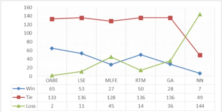
In contrast, OABE showed better performance than LSE for the other two small datasets (NASA and Telecom) that do not have categorical features. To summarize the results we run the win-tie-loss algorithm to show the overall performance. Figure 3 shows the sum of win, tie and loss values for all models, over all datasets. Every model in Figure 2 is compared to other five models, over six error measures and eight datasets. Notice in Figure 2 that except the low performing model on, the tie values are in 49-136 band. Therefore, they would not be so informative as to differentiate the methods, so we consult win and loss statistics to tell us which model performs better over all datasets using different error measures.
Apparently, there is significant difference between the best
and worst models in terms of win and loss values (in the extreme case it is close to 119). The win-tie-loss results offer yet more evidence for the superiority of OABE over other adjustment techniques. Also the obtained win-tie-loss results confirmed that the predictions based on OABE model presented statistically significant but necessarily accurate estimations than other techniques.
Two aspects of these results are worth commenting: 1) The NN was the big loser with bad performance for adjustment. 2) LSE technique performs better than MLFE which shows that using size measure only is more predictive than using all size related features.
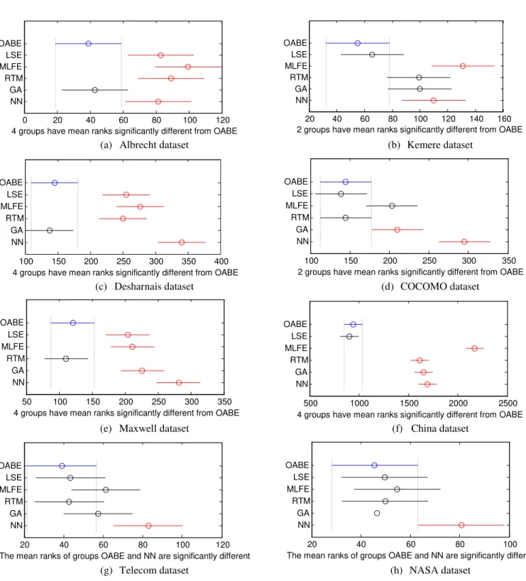
We use the Bonferroni-Dunn test to compare the OABE method against other methods as shown in Figure 3. The plots have been obtained after applying ANOVA test followed by Bonferroni test. The ANOVA test results in p-value close to zero which implies that the differences between two methods are statistically significant based on AR measure. The horizontal axis in these figures corresponds to the average rank of methods based on AR. The dotted vertical lines in the figures indicate the critical difference at the 95% confidence level. Obviously, the OABE methods generated lower AR than other methods over most datasets except for small datasets. For such datasets, all models except NN generated relatively similar estimates but with preference to OABE that has smaller error. This indicates that OABE adjustment method is far less prone to incorrect estimates.
Fig. 2. Win-Tie-Loss Results for all Models
VI. CONCLUSIONS AND FUTURE WORK
This paper presents a new adjustment technique to tune ABE using Bees optimization algorithm. The BA was used to automatically find the appropriate k value and its feature weights in order to adjust the retrieved k closest analogies. The results obtained over 8 datasets showed significant improvements on prediction accuracy of ABE. We can notice that all models’ ranking can change by some amount but OABE has relatively stable ranking according to all error measure as shown in Figure 2. Future work is planned to study the impact of using ensemble adjustment techniques.
VII. ACKNOWLEDGEMENT
(a) Albrecht dataset (b) Kemere dataset
(c) Desharnais dataset (d) COCOMO dataset
(e) Maxwell dataset (f) China dataset
(g) Telecom dataset (h) NASA dataset
Fig. 3. Bonferroni-Dunn test multiple comparison test over all datasets
REFERENCES
[1] M. Azzeh, A replicated assessment and comparison of adaptation techniques for analogy-based effort estimation, Journal of Empirical Software Engineering vol. 17, pp. 90-127, 2012.
[2] M. Azzeh, Y. Elsheikh, Learning Best K analogies from Data Distribution for Case-Based Software Effort Estimation, The Seventh International Conference on Software Engineering Advances (ICSEA 2012), pp. 341-347, 2012.
[3] G. Boetticher, T. Menzies, T. Ostrand, PROMISE Repository of empirical software engineering data http://promisedata.org/ repository, West Virginia University, Department of Computer Science. 2012.
[4] N. H. Chiu, S. J. Huang, The adjusted analogy-based software effort estimation based on similarity distances, Journal of System and Software, Vol. 80, pp. 628–640, 2007.
[5] A. Idri, A. Abran, T. Khoshgoftaar, Fuzzy Analogy: a New Approach for Software Effort Estimation, 11th International Workshop in Software Measurements, pp. 93-101, 2001.
[6] M. Jorgensen, U. Indahl, D. Sjoberg, Software effort estimation by
analogy and “regression toward the mean”, Journal of System and
Software, vol. 68, pp. 253-262, 2003.
[7] C. Kirsopp, E. Mendes, R. Premraj, M. Shepperd, An empirical analysis of linear adaptation techniques for case-based prediction, Internation
20 40 60 80 100 NN
GA RTM MLFE LSE OABE
The mean ranks of groups OABE and NN are significantly different 20 40 60 80 100 120
NN GA RTM MLFE LSE OABE
The mean ranks of groups OABE and NN are significantly different
500 1000 1500 2000 2500 NN
GA RTM MLFE LSE OABE
4 groups have mean ranks significantly different from OABE 50 100 150 200 250 300 350
NN GA RTM MLFE LSE OABE
4 groups have mean ranks significantly different from OABE
100 150 200 250 300 350 NN
GA RTM MLFE LSE OABE
2 groups have mean ranks significantly different from OABE 100 150 200 250 300 350 400
NN GA RTM MLFE LSE OABE
4 groups have mean ranks significantly different from OABE
20 40 60 80 100 120 140 160 NN
GA RTM MLFE LSE OABE
2 groups have mean ranks significantly different from OABE 0 20 40 60 80 100 120
NN GA RTM MLFE LSE OABE
conference on Case-Based Reasoning Research and Development, pp. 1064-1064, 2003
[8] E. Kocaguneli, T. Menzies, A. Bener, J. Keung, Exploiting the Essential Assumptions of Analogy-based Effort Estimation, Journal of IEEE transaction on Software Engineering, vol. 38, pp. 425-438, 2011. [9] J. Z. Li, G. Ruhe, A. Al-Emran, M. Richter, A flexible method for
software effort estimation by analogy, Journal of Empirical Software Engineering, vol. 12, pp. 65–106, 2007.
[10] Y. F. Li, M. Xie, T. N. Goh, A study of A study of the non-linear adjustment for analogy based software cost estimation, Journal of Empirical Software Engineering, vol. 14, pp. 603–643, 2009.
[11] U. Lipowezky, Selection of the optimal prototype subset for 1-nn classification, Pattern Recog. Letters, vol. 19, pp. 907–918, 1998. [12] E. Mendes, N. Mosley, S. Counsell, A replicated assessment of the use
of adaptation rules to improve Web cost estimation, International Symposium on Empirical Software Engineering, pp. 100-109, 2003.
[13] I. Myrtveit, E. Stensrud, M. Shepperd, Reliability and validity in comparative studies of software prediction models, Journal of IEEE Transaction on Software Engineering, vol. 3, pp. 380–391, 2005. [14] D. T. Pham, A. Ghanbarzadeh, E. Koç, S. Otri , S. Rahim, M. Zaidi, The
Bees Algorithm – A novel tool for complex optimisation problems, Proceedings of the 2nd Virtual International Conference on Intelligent Production Machines and Systems, pp. 454-459, 2006.
[15] M. Shepperd, C. Schofield, Estimating software project effort using analogies, Journal of IEEE Transaction on Software Engineering, vol. 23, pp. 736–743, 1997.
[16] F. Walkerden, D. R. Jeffery, An empirical study of analogy-based software effort Estimation, Journal of Empircal Software Engineering, vol. 4, pp. 135–158, 1999.