Quantitative estimating size of deep defects in multi-layered structures from eddy current NDT signals using improved ant colony algorithm

(1)

B. Ye et alii, Frattura ed Integrità Strutturale, 28 (2014) 32-41; DOI: 10.3221/IGF-ESIS.28.04

Quantitative estimating size of deep defects in multi-layered

structures from eddy current NDT signals using improved ant

colony algorithm

Bo Ye, Ming Li, Gefei Qiu, Jun Dong, Fang Zeng

Faculty of Electric Power Engineering, Kunming University of Science and Technology

yeripple@hotmail.com, kingttlly@foxmail.com, tsugefei@foxmail.com, yn_dj@tom.com fanger1119@163.com

Tanghua Yang, Biao Bai

Puer power supply bureau, Yunnan Power Grid Corporation aiyi2001@sina.com, baibiao2014@hotmail.com

ABSTRACT. Detection and quantitative estimation of deep defects in multi-layered structures is an essential task

in a range of technological applications, such as maintaining the integrity of structures, enhancing the safety of aging aircraft, and assuring the quality of products. A novel approach to accurately quantify the two-dimensional axisymmetric deep defect size from eddy current nondestructive testing (NDT) signals is presented here. The method uses a finite element forward model to simulate the underlying physical process and an improved ant colony algorithm (IACA) to solve the inverse problem. Experiments are carried out. The performance comparison between the IACA method and the least square method is shown. The comparison results demonstrate the feasibility and validity of the IACA method. Between them, the IACA method gives a better estimation performance than the least square method at present.

KEYWORDS. Eddy current nondestructive testing; Finite element method; Ant colony algorithm; Multi-layered

structures; Defect measurement.

INTRODUCTION

ulti-layered structures are widely used in many different structural systems, such as nuclear structures, composite aircraft structures, and other civil engineering structures [1]. Structural integrity is one of the prime requirements for multi-layered structures in working condition. The continuous operation of multi-layered structures leads to the loss of its material due to defect generation [2, 3]. The generation of defects in the structure does not mean that structure is at the end of its service life; it becomes necessary to check the multi-layered structure integrity to ensure optimal utilization to its service life. To check the multi-layered structures, various nondestructive testing (NDT) techniques are used, such as visual inspection, eddy current (EC) technique, ultrasonic technique, X-rays, etc. Among these NDT techniques, the eddy current nondestructive testing (ECNDT) method is a useful technique for detecting defects in conductive materials, especially in multi-layered structures. When using the other NDT techniques [4-8], it is widely recognized as being both a complex and critical problem.

(2)

In ECNDT, one of the principal challenges is to determine the size of deep defects in the multi-layered structures based on information contained in the signal representing the change in impedance of the coil as it scans over the specimen. For single-layered structure materials, the high degree of accuracy of some numerical simulation techniques has been demonstrated and several fast computational methods have been presented [9-11]. However, the quantitative estimating size of deep defects in multi-layered structures still poses a major challenge and remains to be dealt with [12].

In this paper, we propose a method of inversing eddy current NDT signals to quantify deep defect size using an iterative improved ant colony algorithm (IACA). The forward problem is calculated via the finite element method (FEM). This method simplifies the inversion process and can be used more easily for complicated defects owing to the flexibility of finite elements. The accuracy and robustness of dimensional (2D) estimation results for a deep defect in the two-layered structures demonstrate the potential of implementing the algorithm.

PROBLEM DESCRIPTION

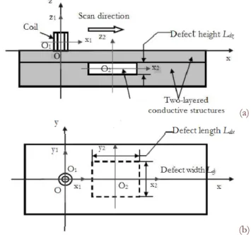
he arrangement for the detection problem of the two-layered structures using the ECNDT technique is shown in Fig. 1. The typical deep defect investigated in this work is assumed to be a regular rectangle defect with different values of length, height and depth, representing the model of a real inner deep defect increasing in time and size. The ECNDT system taken into account here has been developed in our laboratory. The right-cylindrical air-cored coil probe scans over the surface of the structures from left to right under testing.

(a)

(b)

Figure 1: Schematic diagram of the detection system. (a) Sectional view; (b) Top view.

In order to describe and calculate the defect size conveniently, Cartesian coordinates are used. The global coordinates are O (x, y, z) and the origin lies in the upside of the two-layered structure surface. The local coordinates of the coil are O1

(x1, y1, z1) and the origin O1 is (0, 0, ½(l2−l1)) in the global coordinates. (l2−l1) is the length of the coil, l2, l1 respectively

represent the global coordinates of the upper and lower side of the coil. The local coordinates of the defect are O2 (x2, y2,

z2) and the origin O2 is assumed the geometry centre of the defect.

FORWARD PROBLEM

he EC problem can be described mathematically by the partial differential equations in terms of the magnetic vector potential. The FEM based on variation principles can obtain the numerical solution of magnetic field by transforming the partial differential equations into the liner algebraic equations, which are built by combining the

T

(3)

The energy functional of magnetic vector potential (step A)

For simplifying analysis, we assume the existing current of coil uniformly distributes at its window, not considering the harmonic component. The conductivity and permeability can vary from layer to layer, but are constant in each one. After magnetic vector potential A (B=×A) is introduced, the Maxwell equation is

2_A₊_k2_A₌−μ_J_s ₍₁₎

where A represents magnetic vector potential, k2₌−_jωμ_{( +}_jωε_),_j_{is an imaginary unit,}ω_{is the angular frequency of}

excitation current (rad), ω=2πf, f is the frequency of excitation current (Hz), Js is the density of excitation current (Amp/m2_{), is the electrical conductivity (S/m),}μ_{is the magnetic permeability of the media involved (H/m), and}ε_is

dielectric constant (F/m).

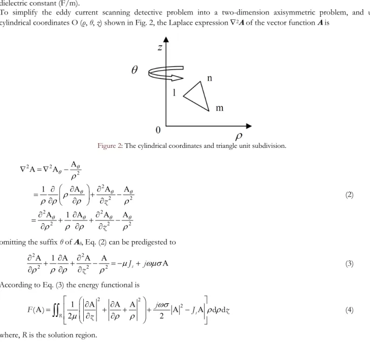
To simplify the eddy current scanning detective problem into a two-dimension axisymmetric problem, and using cylindrical coordinates O (ρ, θ, z) shown in Fig. 2, the Laplace expression 2_A_{of the vector function}_A_is

Figure 2: The cylindrical coordinates and triangle unit subdivision.

2 2

2

2 2

2 2 2

A

A A

A A A

1

A 1 A A A

z

 

  

   



   

 

   

   



 _ _ 

 _  _ 

  

   



 

₍₂₎

omitting the suffix θ of Aθ, Eq. (2) can be predigested to

2 2

2 2 2

A 1 A A A

A s

J j

z  

 

  

     



  (3)

According to Eq. (3) the energy functional is

2 2

2

1 A A A

A A A

2 2

( ) _s d d

R

j

F J z

z

 _{ }

  

  _ _  

   

    

   

 _ _ 

 



₍₄₎

where, R is the solution region.

The solution region (step B)

(4)

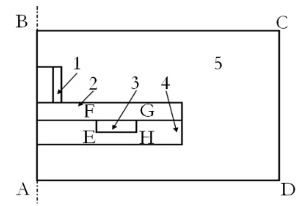
Figure 3: The solution region of FEM: 1-probe 2-aluminum plate 3-defect 4-aluminum plate 5-air region.

Region boundary condition (step C)

The solution region boundary AB, BC, AD and CD are the first boundary. AB is the symmetric axis and the source current is opposite on both sides. The magnetic vector potential A equals to zero along the symmetric axis AB. The boundary of region 5 BC, AD and CD are independent boundary whose magnetic vector potential A is given to zero.

The solution region discretization (step D)

Several principles of triangle subdivision are as follows: 1) Avoiding triangle aspect ratio oversize;

2) Only one species of media in one triangle region, subdivision element is incapable of spanning boundary in the defect region 3 whose boundary is EFGH;

3) Subdivision region denser in the large gradient field, while more sparse in the small gradient field.

Inside any unit shown in Figure 2, adopting linear interpolation function, the magnetic vector potential AP(ρ, z) of any point

P(ρ, z) can be represented using the magnetic vector potential Al, Am and An of the triangle peak points l, m and n.







  

A S S S A A A S A

( , )

T T

P z  l m n l m n  _e (5)

where, AP(ρ, z) is the magnetic vector potential of any point P, the T and e of [A]eT respectively represent transpose and the

finite element, Si is basic interpolation function, namely form function, i=l, m, n, Δ is triangular unit area.

The minimum of energy functional and the finite element equations of magnetic vector potential (step E)

By the first order partial derivative of Eq.5 inside the element, it is expressed: A

A 1 1

A B A

2 2

A

A 1 1

A C A

2 2 A ( ) [ ][ ] ( ) [ ][ ] l T

l m n m e

n

l

T

l m n m e

n

b b b

c c c

z      _  _       _ _  _       _  _  _ _   _      _    ₍₆₎

Based on Eqs. (4), (5) and (6), the energy functional Fe₍_A_{) of every element is:}

  



  



  

2 2

2

1 1 1 1

A C A B A S A S A S A

2 2 2 2

( ) d d

e

T T T T T

e

e e e e e

j

F  J   z

     _ _   _  _   _ _ _ _  _   _           _ _ 



(7)

If the whole solution region is dispersed to M triangular element, the total energy functional of solution region is

1 A A ( ) ( ) M e e F F 

(5)

The computation of FEM equations (step F)

The step A to step E above is the solution procedure of the Ritz law finite element analysis for the EC detection forward problem. From the method, we can obtain the approximate solution of the vector [A] and then the probe impedance changes.

The multi-turn coil, if its density is nc and cross-section is dispersed to K unit element, the impedance of coil is:

2

1 1

2 2

A A

K K

c

ck k ck ck k ck

k k

j n j J

Z r r

I I

   

 





 



 ₍₉₎

where, Δk is triangular element area of the coil interface, rck is distance from the element centroid to symmetric axis, Ack is the A at centroid, and J=ncI is current density of coil.

In this way, on the basis of magnetic vector potential of each node, we can compute the impedance changes of probe.

INVERSE PROBLEM AND IMPROVED ANT COLONY ALGORITHM

uring the last decades, some optimization algorithms, such as artificial neural network, genetic algorithm and artificial immune algorithm, have been successfully applied to solve complex optimization problems in ECNDT. Ant colony algorithm is another heuristic search algorithm succeeding artificial neural network, genetic algorithm and artificial immune algorithm. It is a bionic natural optimization algorithm based on research of foraging behaviors of a real ant colony. It has characteristics of probability seeking and adopts the catalytic mechanism of parallelism and positive feedback. Ant colony algorithm has strong robustness and an excellent distributed computing mechanism. It is easy to combine with artificial neural networks, genetic algorithm, artificial immune algorithm and particle swarm optimization algorithm. However, when solving the continuous domain optimization problems, Ant colony algorithm has the disadvantages of slow convergence and is time consuming in the process of evolution [13, 14]. This paper presents an improved ant colony algorithm (IACA) and proposes the use of IACA to quantitative estimate defect size from EC inspection signals. The IACA has more global search capability and robustness, and ease of implementation.

In order to use IACA, the first step is object discretization as shown in Figure 4. Every vertical line represents a parameter variable. All vertical lines are divided into N equal divisions. The discretization nodes represent the specific values of the parameter variable. Ants walk from the node “start” and pass through the node of every parameter variable. After reaching the node “end”, the IACA completes one cycle and gets a combination of values of all parameter variables. Assuming (r, i) is the ith node of parameter r, xr, j is the value of (r, i). (r +1, j) is the jth node of parameter r +1. [( r, 1) , ( r

+ 1) , j] represents the line connecting node (r, i) and node (r + 1, j). The amount of ants is m. In the process of evolution, ant k (k=1,2, …, m) selects the walk direction according to the pheromone of each path. At time t, the probability of ant k from position (r, i) to position(r + 1, j) is

1 [( , ),( 1, )] [( , ),( 1, )] 0

arg max {[ ( )] [ ( )] }

otherwise

r

j M r i r j t r i r j t q q

s S

 

 



  

  

  

 (10)

where, Mr+1 is the allowable range of the r + 1th parameter, [( , ),(r i r1, )]j ( )t is the intensity of pheromone trace on path [( r, i), ( r + 1), j] at time t. Initially, the intensity of pheromone of each path is equal. _{[( , ),(}_{r i} _r1_{, )]}_j ( )0 C, C is constant.

1

[( , ),(r i r , )]j ( )t

  is visibility of pheromone trace on path [( r, i) , ( r + 1) , j]. It’s is

1

1 1 1

[( , ),( , )]

min

( )

( , ) ( )

r i r j t

J r j J r

   _ _ _ _ (11)

where, J(r + 1, j) is the heuristic function value of different node, Jmin (r +1) is the minimum of J(r + 1, j) in jMr+1. When

the ant selects the path, is the important degree index of the intensity of pheromone trace, while is the important degree index of the visibility of pheromone trace. ≥0, ≥ 0. q is random number, q[0, 1 ]. q0 is a parameter, 0≤q0≤1. S

is the next node selected according to the probability shown in Eq.12.

(6)

B. Ye et alii, Frattura ed Integrità Strutturale, 28 (2014) 32-41; DOI: 10.3221/IGF-ESIS.28.04 1 1 1 1 1 1 1 [( , ),( , )] [( , ),( , )] [( , ),( , )] [( , ),( , )] [( , ),( , )] [ ( )] [ ( )] ( ) [ ( )] [ ( )] r

r i r j r i r j k

r i r j M

r i r j r i r j j t t P t t t                



₍₁₂₎

In the process of creating solution, ants visit each node and update the pheromone using local pheromone along the path.

1 1 1 1

new old

[( , ),(r r , )]j ( )[( , ),(r i r , )]j

          (13)

where, ρ is the decay parameter of pheromone, 0<ρ< 1. Letbe Δ=0=C, 0 is the initial pheromone. After all ants walk

through all nodes, the global pheromone is updated as: 1 1 1 1 1 1 1

[( , ),( , )] min gb

[( , ),( , )]

( ) ( )

if[( , ),( , )] global-best-tour

( )

otherwise r i r j

r i r j

f

r i r j

                          ₍₁₄₎

where fmin gb is the value of objective function at the beginning of iteration. In addition, for continuous domain object,

stochastic search leads to low solution efficiency and solution result dispersion. This paper combines the stochastic search and the deterministic search. After each iterating, ants need to move using the deterministic search strategy. They will then gradually move to the optimal solution. If the solution is worse at this node, the distance of the deterministic moving is longer. At time t, the deterministic moving principle of node (r, i) is:

1 best , , , , _best , , , if if t t

r i r i r i r t

r i _t _t

r i r i r i r

X X X X

X

X X X X

           ₍₁₅₎ min ( , )

, max min

r i r r i r r f f X e f f   

 (16)

where X_rbest is the optimal solution of parameter r at present, e is step size, f(r, i) is the minimum value finding in the

process of passing through the node (r, i). When the feasible scheme is not obtained, f_{( , )}_{r i}  f_rmin. f_rmin is the minimum value of all nodes for parameter r, while f_rmax is the maximum value of all nodes for parameter r. By the nodes moving, nodes will gradually move to the optimal solution. The precision of search results is improved. Until to all r,

, ,

t t r i r j

X X e, that is to say the distance of arbitrary two nodes of all parameters is less than e, which shows that the algorithm is convergence. At that time, the search range has focused near the optimal solution. The optimal solution of parameter r is X_rbest. The iteration will stop. In addition when the cumulative times t of search moving is greater than the maximum moving times tmax the algorithm will stop iteration. In the process of iteration, the deterministic search

continuously modified the moving path. It will be helpful to overcome the disadvantage of result discretization and improve the global optimization capability. Therefore, the IACA can obtain the high precision results and need not to set too large N. Its application to large-scale optimization problems can be easily implemented on parallel machines resulting in a significant reduction of required time.

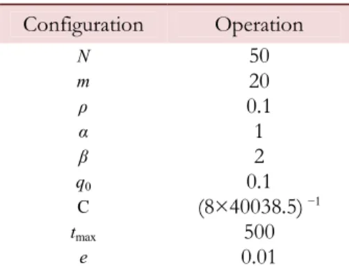
In common, the IACA is conducted according to the following procedure: Step 1 Parameter initialization, parameter equal division (N).

Step 2 m ants walk from the node “start”. According to Eq.10 and Eq.12, every ant individually computes the transition probability and creates the parameter scheme.

Step 3 Compute and save the object function value of feasible scheme, and save the optimal scheme at present.

Step 4 Update the pheromone according to Eq.13 and Eq.14 using the path of the ant associated with the feasible scheme. Step 5 Each node deterministically moves according to Eq.16.

Step 6 _t _t 1_{, If to every parameter r,}

, ,

t t r i r j

X X e, or t≥tmax, then output the optimal scheme. Otherwise, return

(7)

In ECNDT, the problem of quantifying defect size from probe signals is formulated as an optimization problem, which seeks a set of defect size by minimizing an objective function, representing the difference between the models predicted signal and the measured signal. The inversion process iteratively attempts to estimate a set of defect size so that the corresponding model predicted signal matches the measured signal.

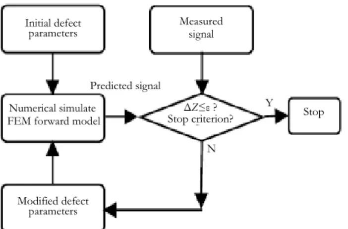
Such method presented by this paper is based on the underlying physical process. A time-varying current flowing into an exciting coil placed near to the specimen induces eddy current in the specimen under testing. The induced eddy current, depending on the spatial values of the resistivity and magnetic permeability, affects the signal detected by the surrounding pick-up coils or magnetic sensors. Then, changes in impedance of the coil are used as a basis for detecting the presence of discontinuities in the specimen by inversion of the measured data. The inversion process is shown in Fig. 4.

Figure 4: The flowchart of quantitative estimating size of deep defects in multi-layered structures from ECNDT signals using IACA.

The measured signal at the position of the defect is assumed the target signal. A set of randomly generated initial defect parameters are given to the finite element model to predict the eddy current coil responses associated with these defects. Then, the model predicted signals are compared with the measured signal and the corresponding value of the objective function is evaluated. If the value of the objective function is less than a predefined threshold, the iterative process is terminated. Otherwise the IACA correct the defect parameters. Then the process is iterated until the error becomes less than the predefined threshold.

NUMERICAL AND EXPERIMENTAL RESULTS

o use IACA in optimization, it is essential to settle the configuration of many parameters. Parameter equal division number (N), ant number (m) and maximum moving times (tmax) are heuristically determined and dependent on the

optimization problem.

In the method with the help of IACA applied to determinate the parameters of the defect, the length, the height and the depth of the defect are expressed as:

X=[l, h, d] (17) where, l is the length of the defect, h is the height of the defect; d is the depth of the defect. The object function is:

2 1

1

1 g '

i i i

f

a _ z z









(18)

where, a is a constant, zi is the model predicted coil impedance at scanning position i, and zi’ is the corresponding probe impedance from actual measurement. g is the number of scanning positions. The object function is calculated by comparing the signals of the measurement with those of the prediction by FEM forward model. Updating the pheromone and deterministically moving are operated based on the object function value. After a lot of iteration, the ant with the highest object function value is expected to indicate the defect size. The other features of IACA which are used in this paper are shown in Tab. 1. The structure parameters are shown in Tab. 2 and the coil parameters are shown in Tab. 3.

T

N Predicted signal

Stop Initial defect

parameters

Numerical simulate FEM forward model

ΔZ≤ε ? Stop criterion?

Y Measured

signal

(8)

Configuration Operation

N 50

m 20

ρ 0.1

α 1

β 2

q0 0.1

C _(8×40038.5)−1

tmax 500

e 0.01

Table 1: IACA configuration.

Structures Conductivity _σ MS/m

Permeability μ

Thickness

tmm

Layer 1 18.5 μ0 1

Layer 2 18.5 μ0 2

Defect 0 μ0

Table 2: Structure parameters.

Item Quantity

Number of turns N 330

Inside radiusr1mm 3.0

Outside radiusr2mm 5.11

Lengthlmm 20.70

Inductance L0mH 1.02

ResistanceR0Ω 19.84

Frequencyf0Hz 400

Liftoff l1mm 0.0

Table 3: Coil parameters.

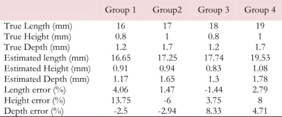
In the actual computing process, we find the method needs a long computing time to find the global optimum, when the estimation of the objective function requires a field analysis by means of the FEM. So, we propose a novel method with a signal database consisting of impedance signals of different size computed by FEM in advance, applied to the optimization of defect inspection, to reduce the computing time for the whole optimization. The identification results using IACA are shown in Tab. 4. At the same time, the identification results using the least square method are shown in Tab. 5.

Group 1 Group2 Group 3 Group 4

True length (mm) 16 17 18 19

True Height (mm) 0.8 1 0.8 1

True Depth (mm) 1.2 1.7 1.2 1.7

Estimated length (mm) 16.26 17.16 17.83 18.74

Estimated Height (mm) 0.84 1.04 0.77 1.04

Estimated Depth (mm) 1.22 1.73 1.15 1.66

Length error (%) 1.63 0.94 -0.94 -1.37

Height error (%) 5 4 -3.75 4

(9)

Group 1 Group2 Group 3 Group 4

True Length (mm) 16 17 18 19

True Height (mm) 0.8 1 0.8 1

True Depth (mm) 1.2 1.7 1.2 1.7

Estimated length (mm) 16.65 17.25 17.74 19.53 Estimated Height (mm) 0.91 0.94 0.83 1.08

Estimated Depth (mm) 1.17 1.65 1.3 1.78

Length error (%) 4.06 1.47 -1.44 2.79

Height error (%) 13.75 -6 3.75 8

Depth error (%) -2.5 -2.94 8.33 4.71

Table 5: Identification of defect using the least square method.

Comparing Tab. 4, using IACA, and Tab. 5, using the least square method, the results show that the former has higher precision and robustness than the latter.

CONCLUSION

n iterative improved ant colony algorithm has been implemented with FEM to determine the defect size in ECNDT. Defect size is automatically obtained and material parameters of the structure can be obtained more effectively than the existing ECNDT method. The main advantage of this method is its easy implementation. Particularly, the resolution of FEM has been pre-calculated. The only work is to write a few lines of code in order to define parameters to be optimized, the objective function and the constraints. The improved fast inverse method with the database computed in advance distinctly reduces the computing time of the whole optimization. The possibility of quantifying size of deep defects in multi-layered structures is demonstrated. A decrement in human errors and faster inspections can be expected by completely automatic inspection.

ACKNOWLEDGMENT

his work is supported by the National Natural Science Foundation of China Grant No. 51105183, the Research Fund for the Doctoral Program of Higher Education of China Grant No. 20115314120003, the Applied Basic Research Programs of Science and Technology Commission Foundation of Yunnan Province of China Grant No. 2010ZC050, the Foundation of Yunnan Educational Committee Grant No. 2013Z121, the National College Student Innovation Training Program Funded Projects Grant No. 201210674014, the Science and Technology Project of Yunnan Power Grid Corporation Grant No. K-YN2013-110.

REFERENCES

[1] Takagi, T., Huang, H., Fukutomi, H., Tani, J., Numerical evaluation of correlation between crack size and eddy current testing signal by a very fast simulator, IEEE Trans. Magn., 34 (1998) 2581–2584.

[2] Auld, B.A., Moulder, J.C., Review of advances in quantitative eddy current nondestructive evaluation, J. Nondestr. Eval., 18 (1999) 3-36.

[3] Ye, B., Cai, J., Huang, P., Fan, M., Gong, X., Hou, D., Zhang, G., Zhou, Z., Automatic classification of eddy current signals based on kernel methods, Nondestruct. Test. Eva., 24 (2009) 19-37.

[4] Mandache, C., Khan, M., Fahr, A., Yanishevsky, M., Numerical modelling as a cost-reduction tool for probability of detection of bolt hole eddy current testing, Nondestruct. Test. Eva., 26 (2011) 57-66.

[5] Shubochkin, A.E., Eddy-current testing of the quality of railway wheels, Russ. J. Nondestruct. Test., 41 (2005) 189-192.

[6] Kojima, F., Fujioka, T., Quantitative evaluation of material degradation parameters using nonlinear magnetic inverse problems, Int. J. Appl. Electrom., 25 (2007) 57-163.

A

(10)

[7] Fitzpatrick, G.L., Thome, D.K., Skaugset, R.L., Shih, E.Y.C., Shih, W.C.L., Magneto-optic/eddy current imaging of aging aircraft: a new NDI technique, Mater. Eva., 51 (1993) 1402-1407.

[8] Thollon, F., Lebrun, B., Burais, N., Jayet, Y., Numerical and experimental study of eddy current probes in NDT of structures with deep flaws, NDT&E Int., 28 (1995) 97-102.

[9] Chomsuwan, K., Yamada, S., Iwahara, M., Improvement on defect detection performance of PCB inspection based on ECT technique with Multi-SV-GMR sensor, IEEE Trans. Magn., 43 (2007) 2394-2396.

[10]Edward, P., Manson, J., The application of dual-frequency eddy current inspection to aircraft structures, Insight, 44 (2002) 141-145.

[11]Zenzinger, G., Bamberg, J., Satzger, W., Carl, V., Thermographic crack detection by eddy current excitation, Nondestruct. Test. Eva., 22 (2007) 101-111.

[12]Huang, L., He, R., Zeng, Z., An extended iterative finite element model for simulating eddy current testing of aircraft skin structure, IEEE Trans. Magn., 48 (2012) 2161–2165.

[13]Dorigo, M., Gambardella, L.M., Ant colony system: a cooperative learning approach to the traveling salesman problem, IEEE Trans. Evolut. Comput., 1 (1997) 53-66.