Vol. 11, No. 4 (special issue), December 2014, 535-549
Defect Detection in Conducting Materials
Using Eddy Current Testing Techniques
Hartmut Brauer
1, Marek Ziolkowski
1, Hannes Toepfer
1Abstract: Lorentz force eddy current testing (LET) is a novel nondestructive testing technique which can be applied preferably to the identification of internal defects in nonmagnetic moving conductors. The LET is compared (similar testing conditions) with the classical eddy current testing (ECT). Numerical FEM simulations have been performed to analyze the measurements as well as the identification of internal defects in nonmagnetic conductors. The results are compared with measurements to test the feasibility of defect identification. Finally, the use of LET measurements to estimate of the electrical conductors under test are described as well.
Keywords: Nondestructive evaluation,eddy current testing, Lorentz force.
1 Introduction
Nondestructive evaluation (NDE) comprises many terms used to describe various activities within the field. Some of these terms are nondestructive testing (NDT), nondestructive inspection (NDI), and nondestructive exami-nation (which is often called NDE as well, but should probably be called NDEx). These activities include testing, inspection, and examination, which are similar in that they primarily involve looking at (or through) or measuring something about an object to determine some characteristic of the object or to determine whether the object contains irregularities, discontinuities, or flaws.
The terms irregularity, discontinuity, and flaw can be used interchangeably to mean something that is questionable in the part or assembly, but specifications, codes, and local usage can result in different definitions for these terms. Because these terms all describe what is being sought through testing, inspection, or examination, the term NDE (nondestructive evaluation) has come to include all the activities of NDT, NDI, and NDEx used to find, locate, size, or determine something about the object or flaws and allow the investigator to decide whether or not the object or flaws are acceptable. A flaw that has been evaluated as rejectable is usually termed a defect.
Nondestructive testing (NDT) is a wide group of analysis techniques used in science and industry to evaluate the properties of a material, component or system without causing damage. Because NDT does not permanently alter the article being inspected, it is a highly valuable technique that can save both money and time in product evaluation, troubleshooting, and research.
Today the increased competition in industry and the expectation of shorter return-of-invest periods for complex and expensive machinery, as well as occupational safety, health and environmental requirements, presuppose a high availability of the production machinery and a high and stable quality of the products. These goals are met only if the machinery is kept in proper working condition by utilizing a functioning maintenance philosophy and the right machine diagnostic methods for preventing machinery breakdowns and loss of profit.
Nondestructive testing methods are all those evaluation methods by which the integrity of different components or assembled pieces of equipment is being examined nondestructively. The examination can be performed directly after manufacturing, during acceptance testing or on-line as a tool for preventive maintenance as well as for the location of damages, the analysis and the after-care of damages. The diagnostic methods utilize physical phenomena to monitor the health of materials or devices and to make prognosis of the future use. This is more-and-more often done online without interrupting the industrial process.
2
Short History of NDT
Before a brief history of the methods can be presented, one has to remember the definition of an NDT-method being one utilizing a physical phenomenon for the noninvasive testing of a product or a material.
With this definition in mind, the oldest NDT-method by far is visual testing (VT) which is as old as mankind starting most likely from the visual checking of knives for cutting meat and spears for hunting [16].
Acoustics would be the second oldest method as it has been used for testing since ancient times when man started to make the first pottery vessels. The earliest known pottery vessels may be those made by the people in China about 20000 years ago [17] and acoustics was surely used much later on for the testing of glassware. The same technique was used in the Middle Ages when testing for instance brass castings such as a huge church bell. This was, however, testing with audible sound.
gun pipes in 1868. Here he utilized the remanence of the steel giving detectable leakage fields.
Magnetic particle testing (MT) was patented in The United States in 1922 when W.E. Hooke, working with precision gage blocks at the American Bureau of Standards, devised a method for magnetizing an object producing a leakage field and using iron powder to delineate cracks invisible to the naked eye. The real breakthrough for magnetic particle testing came, however, about a decade later after F.B. Duane and A.V. de Forest had started a partnership in 1929 that later on in 1934 became the Magnaflux Corporation.
Before the breakthrough of magnetic particle testing the first classical NDT- method was, of course, radiography (RT). Nondestructive testing, the way we define it, started when Professor Wilhelm Conrad Roentgen in 1896. After his discovery of the unknown, i.e. the X-rays, took a radiograph of four soldered pieces of zinc and one of his own hunting rifle. The radiograph of the rifle showed some cast defects in the material and was thus the start of industrial radiography. Professor Roentgen disguised the publicity around him and never made any attempts to claim a patent on his discovery.
The second method to be patented was the penetrant method (PT) when in 1948 F.B. Duane was awarded a patent for the fluorescent penetrant method. Penetrant testing was actually used before magnetic particle testing. The method was formerly called "The oil and whiting method" and was used for testing heavy cast parts used by the huge locomotives in the beginning of the 20th century. They applied used oil that had a dark pigment, i.e. contained dirt, and whiting was simply a water-based chalk-slurry that dried out to white film and worked as the developer.
The basis for ultrasonic testing (UT) was established in 1940 when F.A. Firestone achieved a patent for his invention concerning a flaw detection device. Then in 1942 Firestone was the first to use his method for the sonar. In Germany two physicists and brothers Herbert and Josef Krautkrämer, who had studied works by Firestone, made a bet of being able to tell if a cannonball, too thick to be radiographed with existing equipment, would have a casting flaw inside or not. They used ultrasound transmission for the bet and won the bet. They founded a firm that was to become the biggest ultrasonic testing equipment manufacturer ever. These two German brothers did a lot of research of the method and greatly contributed to the development of the method [18]. Since their time the method has gone through several phases of development and made enormous achievements in many countries and still has great potential for further applications.
materials, but a working theory of the method was lacking. Then, it was the German F. Foerster who in the 1950s clarified the theory for Eddy Current Testing and devised the necessary formulae [19]. Today production testing of austenitic tubes and in-service testing of heat-exchanger tubes are well known applications of eddy current testing.
A somewhat more recent method finding new applications is the acoustic emission method (AE). The basis for the method lies in the Kaiser-effect discovered by the German Professor J. Kaiser in 1950 [20]. He noticed that the material emits sound in the ultrasound region when discontinuities are developing while straining over the former highest strain level the material has been exposed to. In other words, if a crack is not propagating, it does not emit sound and is thus fairly non-critical, but as the emission starts and rises the cracks are propagating. The emission for emitting areas can be tracked in huge components seismographically and other more local NDT-methods can then be applied for dimensioning of the discontinuities. The method has been successfully applied for detecting leaks, propagating cracks and lately also for monitoring the manufacturing processes for abnormal emissions. An example of this would be the monitoring of a continuous casting machine in a steel factory or a timber chopper in a pulp and paper mill.
The actual breakthrough for the use of NDT-methods took place during the Second World War starting from the testing of submarines and airplanes. During these good fifty years the use has then incorporated the inspection of nuclear power plant components, pressure vessels, bridges, elevators and car parts, which if measured in numbers is the biggest user today.
3
Eddy Current Testing
In short, one could claim that primarily the idea of using NDT-methods is to find discontinuities in the material, either originating from the manufacturing process or from overstraining in use. The sought discontinuities are mostly cracks stemming from false manufacturing techniques or from fatigue or thinning caused either by corrosion or erosion.
In other words, first the discontinuities have to be located. Thereafter the dimensions and directions of the discontinuities have to be measured, after which the flaws are to be evaluated for conformance to stipulated acceptance criteria. These criteria evolve from fracture mechanical calculations based on critical flaw size and the speed of the extension of the flaw.
have been the prerequisites for the development of an actually widespread electromagnetic testing technique, the eddy current testing (ECT).
Faraday has found that due to the relative movement of a conductor and a magnetic field, a voltage is induced in the conductor, causing a current flow. This means, that exerting of an alternating magnetic field of a coil leads to an induced voltage in a conducting specimen, driving a current flow in the test object. Thus, the electromagnetic induction is the working principle of the ECT which can be applied to nondestructive testing of conducting materials only.
In 1834, Heinrich Hertz formulated the principle that the properties of the test object react on the test system. The Lenz law describes that the current flow in the test object is directed in a way that the magnetic field caused by this current is counteracting the primary magnetic field. Thus, eddy currents cause a secondary magnetic flux in the test coil which is compensating that part of the flux in the coil that is equivalent to magnitude and phase of the flux caused by the eddy currents. But these eddy currents have first been “invented” by James Clerk Maxwell as he formulated in 1864 the equations defining the theory of the electromagnetic fields. The utilization of eddy currents was done by D.E. Hughes in 1879 for the first time while testing methods of ore sorting.
The development of eddy current testing was growing up significantly as Dr. Friedrich Foerster founded the Institut Dr. Foerster (1948). In the late 1960s, this Institute developed several ECT devices for industrial applications. The next important milestone was the introduction of the multi-frequency technique by the French manufacturer Intercontrolle of France in 1974. Later several special techniques have been developed (e.g. magnetic flux leakage, remote eddy current testing, modulation analysis inspection, etc.) leading to a remarkable extension of the spectrum of practical applications.
All these techniques working on the same principle, where a coil driven by an alternating current induce eddy currents in the conducting specimen, which distribution in the material enables some estimation of its properties, similar advantages and disadvantages can be expected. The frequency-dependent penetration depth of the electromagnetic field in the conductor as well as the low spatial resolution for low frequencies are limiting the identification of deep internal defects in the test object. Consequently, ECT can be considered as a surface-oriented method which enables preferably the detection of flaws at the surface or close to the surface. Additionally, metallic alloys or wall and coating thicknesses can be estimated with ECT as well.
verify different material parameters, like electrical conductivity, magnetic permeability, detection of discontinuities, material thickness or coating thickness of metallic objects, the effect of the distance between test coil and test object (lift-off distance) or the distances of conductors in laminated materials (e.g. composites). The result is a wide spectrum of applications for the ECT methods, from the pipe inspection in power plants, in the chemical or petrochemical industry, in nuclear submarines or air conditioning devices via the inspection in aircraft and automotive industries through the manufacturing of pipes, wires, rods and bars.
4
Lorentz Force Eddy Current Testing
Nondestructive Testing (NDT) and Evaluation (NDE) of electrically conductive objects require reliable methods to detect material anomalies or deep lying defects. Besides of radiographic, ultrasonic or optical techniques, electromagnetic methods such as eddy current testing (ECT) find a wide range of application due to low cost, easy to use equipment and low demands to the measurement environment [8, 9]. However, one of the most limiting factors in ECT is the frequency dependent skin depth [6]. This restricts the capability to detect deep lying defects. With Lorentz force eddy current testing (LET) a novel electromagnetic nondestructive testing technique is presented [4, 11-13]. The aim is to overcome this limitation.
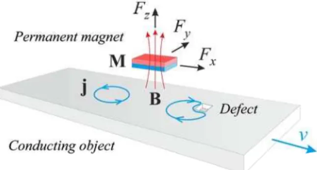
Lorentz force eddy current testing is based on setting an electrically conductive specimen into relative motion to a constant magnetic field. Due to Ohm’s law for moving conductors, eddy currents are induced in the conductor under test
t
A
j v B , (1)
where j denotes the induced current density, φ the scalar electric potential, A the magnetic vector potential (B = ×A, A = 0), v the conductor velocity, and B the total magnetic flux density. B can be divided into a primary magnetic field (caused by a permanent magnet) and a secondary magnetic field generated by the eddy currents.
The interaction of the constant magnetic field and the induced eddy currents results in a Lorentz force FL acting on the specimen. Due to Newton´s
third law, an equal force FPM exerts on the permanent magnet in the opposite
direction (Fig. 1)
d
C
PM L
V
V
with VC describing the volume of the specimen. If a defect is present in the
conductive material, perturbations in the measured Lorentz force occur. Based on these perturbations the defect can be detected and perhaps be reconstructed.
Fig 1 – Basic principle of LET. The conductive specimen moves with velocity v relative to a permanent magnet. The interaction between the primary magnetic field and the induced eddy
currents in the specimen results in Lorentz force components Fx, Fy and Fz exerted on the permanent magnet.
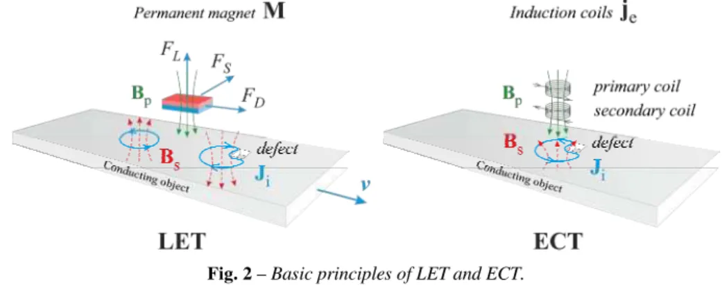
In contrast to LET, common eddy current testing uses a time changing current in a primary coil which generates a time changing primary magnetic field Bp. Usually, the signal used to evaluate the material, is the change in
impedance of the secondary coil.
Both principles are based on the induction of eddy currents, whereas major differences arise in shape and magnitude of the induced current densities as well as in the method of signal evaluation. Fig. 2 shows the comparison of both methods and illustrates the perturbation of eddy currents due to defects. Normalized force perturbations (LET) and impedance perturbations (ECT) are illustrated in Fig. 4. The graph shows normalized signals of the drag-force Fx
together with the imaginary part of the secondary coil impedance at comparable source dimensions (PM vs. coil).
In both methods, a secondary magnetic field Bs is generated which interacts
with the primary magnetic field Bp. The total magnetic field is given by the sum
of both fields B = Bp + Bs. The formalism to describe the LET and ECT problem
in theory is given by the magnetic convection diffusion equation [13, 14], which can be written in its potential form as
0
1
e t
A
A M v A j , (3)
ECT is the skin-depth δ, which results in a fast decay of the information signal for subsurface defects
2
. (4)
A similar factor is defined for moving conductors, namely the magnetic Reynolds number Rm. It can be derived by transforming the magnetic
convection diffusion equation in its non-dimensional form [12]
m
R vL. (5)
The parameter L is the typical length-scale of the problem. In general, for Rm<<1 diffusion of the magnetic field dominates and the resulting field is
primarily determined by the boundary conditions and the primary magnetic field Bp. For Rm >> 1, the magnetic field lines are advected in the moving direction,
which results in a similar phenomenon as skin effect.
Fig. 2 – Basic principles of LET and ECT.
This experimental setup has also been used to perform the numerical simulations. An example of 3D-FEM simulations is shown in Fig. 3b. For numerical simulations the finite element method (FEM) was used to solve the given field problem. Using the A- potential formulation, the LET field problem can be described by (3), but without the external current density on the right-hand side. This formulation separates the two induction phenomena into
the moving part v×B and the time changing part t
A
on the right-hand side.
Depending on the definition of the frame of reference, two equivalent types of the general magnetic field induction equation can be distinguished [13, 14]. In the so-called moving frame of reference, the global coordinate system is associated with the moving permanent magnet, i.e. the conducting object moves in the direction along the x-axis with velocity v. If the conducting object moves with a constant velocity and has a constant cross-section normal to the direction
of motion, e.g. the object is free of defects, the time derivative t
A
vanishes and
(3) is reduced to a quasi-static approach.
(a) (b)
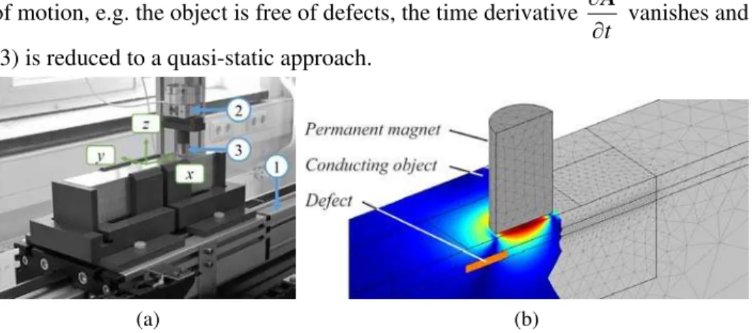
Fig. 3 – (a) Experimental setup with linear drive (1), 3D force sensor (2), permanent magnet (3)
and 2D linear stage (not shown); (b) 3D FEM model used for LET simulations.
It has been shown in experiments, that the detection of subsurface defects in stacked Aluminum sheets is possible for both testing techniques using the described experimental setup [15]. In ECT the detection of subsurface defects is mainly limited by the frequency dependent penetration depth of eddy currents. Thus, the testing frequency has to be chosen as low as possible. But if such low frequencies are used, the performance of the electronic amplifier becomes more important due to the weak signals. Furthermore, the testing speed is strongly restricted depending on the properties of defects, e.g. characteristic length and shape.
In LET, the relative movement between the permanent magnet and the specimen is needed to induce eddy currents. To create a sufficiently large Lorentz force, the relative velocity has to be high enough to detect small perturbations induced by subsurface defects. With increasing speed, the absolute force and the force perturbations increase linearly at magnetic Reynolds number Rm < 1. Therefore, the magnitude of the desired force signal is
theoretically adjustable with the velocity for optimal utilization of the applied force sensor. In practice, the force sensor is sensitive to unwanted vibration of the environment and the system itself. To summarize, both testing techniques are highly dependent on the used sensors and measurement electronics, whereas the available testing speed, and therefore several areas of application for LET and ECT are quite different.
5 Sigmometry
relative motion between a permanent magnet and the conductor under test. This allows the field to penetrate deeper inside the material compared to eddy current techniques under the same conditions [3]. Since the internationally widely used Greek symbol for the conductivity is σ (sigma) and the exploited physical effect is the Lorentz force, this technique has been called ”Lorentz Force Sigmometry” (LoFoS) [4].
5.1 Basic principle
To explain the LoFoS principle a conducting plate of finite cross-section and finite length, moving with constant velocity v across a static magnetic field, denoted by B is assumed. The magnetic field is produced by a permanent magnet which is placed at a lift-off distance δz above the conductor. The magnet is magnetized in the z-axis direction with magnetization density denoted by M. According to the Ohm's law, due to the relative motion between the conductor and a permanent magnet eddy currents j are induced. Due to their interaction with the external magnetic field B, eddy currents further produce a Lorentz force which acts inside the conductor and brakes its relative motion. The total value of the braking force FB can be determined as
d
C B
V
V
F j B , (6)
where Vc is the volume of the moving conductor. The braking effect of the
Lorentz force is well-known. By contrast it is less widely appreciated that by virtue of Newton's third law, a Lorentz force with the same magnitude but with opposite direction acts upon the permanent magnet as well. This phenomenon has already found practical application for the contactless velocity measurement in metallurgy known as “Lorentz force velocimetry” (LFV) and for defect detection in solid metals, where it is called "Lorentz force eddy current testing" (LET) [5]. For the given LoFoS setup, the Lorentz force comprises of only two components, namely the drag force FX and the lift force FZ. The magnitude of
the Lorentz force depends on the electrical conductivity of the material, applied magnetic field, relative velocity and dimensions of the conductor. In order to reduce the number of dependent variables the analysis can be performed in terms of the non-dimensional magnetic Reynolds number defined as Rm =
µ0σvL, where μ0 is the permeability of vacuum and L a characteristic length
scale of the conductor in motion [3, 4]. When Rm is small, it can be shown that
the drag component of the Lorentz force depends linearly on the magnetic Rm,
whereas the lift force component is proportional to the square of Rm [3]:
2 2 2
and
x X m z Z m
F B R F B R . (7)
An obvious idea is to calculate the conductivity using only the drag or the lift component of the Lorentz force. Nevertheless, coefficients αX and αZ depend
magnetization density. The strong dependency on the lift-off distance leads to a very high uncertainty in conductivity measurement. Manufacturing errors and mechanical oscillations can lead by ease to deviations of up to 100μm, which could result in relatively strong Lorentz force deviations. The magnetic field strength of the magnet is usually not given and it is difficult to be determined since magnetization direction and mounting errors have to be taken into account. To overcome disadvantages of using only one force component a modified approach is applied which uses the ratio of the two force components instead, namely lift-to-drag ratio FZ/FX. Based on (2), the lift-to-drag ratio
depends linearly on Rm, i.e. on unknown electrical conductivity as well. It has
also been shown that this approach is independent of the magnetization of the used magnet and that the sensitivity on the lift-off distance variations is considerably reduced. Furthermore, it has been shown that, for moving thin sheets, the lift-off dependency is completely avoided [3]. If we assume that the conductivity is isotropic for a constant velocity, the lift-to-drag ratio can be described as σ = α(FZ/FX), where the calibration coefficient α depends on the
geometry of the magnet and the conductor, on the translational velocity and weakly on the distance between the conductor and the magnet. Since α is a priori unknown, it can be determined numerically or experimentally by calibration with well- described specimens.
5.2 Conductivity measurement
The important issue of the LoFoS and the force measurements is the magnitude of the actual measured force. In order to increase the total Lorentz force acting on a magnet, a smaller lift-off distance δz is preferable. The
disadvantage of such a setup is an increased sensitivity of the Lorentz force to changes in lift-off distance. Apart from good agreement between numerical and experimental results more important to notice is the drastic decrease in sensitivity of the lift-to-drag ratio to changes in lift-off distance. This effect considerably decreases the uncertainty of conductivity measurements.
(a) (b)
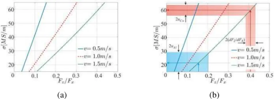
Fig. 5 – (a) Calibration curves for δz = 3mm obtained numerically,
We have also observed that the lift-to-drag force ratio is independent of the magnetization of the used magnet, whereas drag and lift components have quadratic dependency on the strength of the applied external magnetic field [5].
Since electrical conductivity is linearly dependent of the lift-to-drag ratio, the calibration can be done with two points, i.e. two materials (e.g. aluminum and copper). The calibration has to be done for few different velocities for which Rm < 1. Due to the very good agreement between measurements and
numerical results we propose a numerical calibration, where calibration curves are generated by changing the conductivity of the specimen. These calibration graphs can be used to estimate a measured, unknown conductivity (Fig. 5a).
We measured the Lorentz force resulting from two solid specimens of known conductivity, namely aluminum (σAl = 20.4MS/m) and copper
(σCu = 57.92 MS/m) [4]. These conductivities have been measured with the ECT
device Sigmatest 2.069 (Institut Dr. Foerster GmbH & Co. KG). Then, the measured lift-to-drag ratio has been used to determine the conductivity of these conductors using LoFoS. We obtained conductivities of σAl = 21.59MS/m and
σCu = 60.08 MS/m, respectively (Fig. 5b). The combined measurement
uncertainties of uAl = 9.82MS/m and uCu = 3.46MS/m are based on the
uncertainty of the used force sensor (dFX = 15mN, dFZ = 50mN). These
uncertainties can be reduced when the measurements are repeated several times or by applying more accurate force sensors.
6 Applications
to use the results of the research in collaboration with industry for the development of industrial prototypes, which can be commercialized outside the university.
Possible application scenarios are the investigation of weld seams, a defect monitoring of continuous casting setups of conductive material or the defectoscopy at metal injection molding components. Currently the LET method is applied to the defectoscopy at carbon fiber reinforced plastics (CFRP), GLARE, composite materials and other laminated materials
7 Conclusion
In this contribution, a novel electromagnetic nondestructive evaluation technique, the Lorentz force eddy current testing (LET), has been presented. The method enables the detection of subsurface defects in laminated conductive non-ferromagnetic materials. A good agreement of the results with respect to measurements, simulations and reconstruction has been observed. Future investigations are related especially to the improvement of the experimental setup in terms of noise reduction and sensor dynamics. Further numerical simulations will be performed to develop new magnet systems, which will be optimized in terms of resolution. The reconstruction process will be studied continuously by implementing different methods to solve the inverse problem in a fast and accurate manner. Additional investigations will be performed to miniaturize the present setup enabling defect detections in sub-millimeter range.
Furthermore, it can be concluded that the proposed LoFoS technique is able to provide the electrical conductivity of specimen preferably based on volumetric measurements. LoFoS has the following advantages: (i) LoFoS is contactless, (ii) LoFoS can be applied continuously during production processes, (iii) LoFoS is a method that enables the user to measure conductivity below the surface and (iv) the proposed data processing makes LoFoS resistant to changes in lift-off distance, velocity and strength of the magnetic field source. LoFoS is suitable for specimen of any kind of physical condition. The only limitation is due to the minimal measurable Lorentz force components of the used multi-component force sensor.
8 References
[1] N. Bowler, Y. Huang: Electrical Conductivity Measurement of Metal Plates using
Broadband Eddy-current and Four-point Methods, Measurement Science and Technology, Vol. 16, No. 11, Nov. 2005, pp. 2193 – 2200.
[2] B.A. Abu-Nabah, P.B. Nagy: Lift-off Effect in High-frequency Eddy Current Conductivity
Spectroscopy, NDT&E International, Vol. 40, No. 8, Dec. 2007, pp. 555 – 565.
[3] J.R. Reitz: Forces on Moving Magnets due to Eddy Currents, Journal of Applied Physics,
[4] R.P. Uhlig, M. Zec, M. Ziolkowski, H. Brauer, A. Thess: Lorentz Force Sigmometry: A Contactless Method for Electrical Conductivity Measurements, Journal of Applied Physics, Vol. 111, No. 9, May 2012, p. 094914.
[5] A. Thess, E. Votyakov, Y. Kolesnikov: Lorentz Force Velocimetry, Physical Review
Letters, Vol. 96, No. 16, April 2006, p. 164501.
[6] H. Brauer, M. Ziolkowski: Eddy Current Testing of Metallic Sheets with Defects using
Force Measurements, Serbian Journal of Electrical Engineering, Vol. 5, No. 1, May 2008, pp. 11 – 20.
[7] P.C. Hansen: Discrete Inverse Problems: Insight and Algorithms, SIAM, Philadelphia, PA,
USA, 2010.
[8] C. Hellier: Handbook of Nondestructive Evaluation, McGraw-Hill, NY, USA, 2003.
[9] [9] D.C. Jiles: Review of Magnetic Methods for Nondestructive Evaluation (Part 2), NDT
International, Vol. 23, No. 2, April 1990, pp. 83 – 92.
[10] B. Petkovic, J. Haueisen, M. Zec, R.P. Uhlig, H. Brauer, M. Ziolkowski: Lorentz Force
Evaluation: A New Approximation Method for Defect Reconstruction, NDT&E International, Vol. 59, Oct. 2013, pp. 57 – 67.
[11] A. Thess, E. Votyakov, B. Knaepen, O. Zikanov: Theory of the Lorentz Force Flowmeter,
New Journal of Physics, Vol. 9, No. 8, Aug. 2007, p. 299.
[12] R.P. Uhlig, M. Zec, H. Brauer, A. Thess: Lorentz Force Eddy Current Testing: A Prototype
Model, Journal of Nondestructive Evaluation, Vol. 31, No. 4, Dec. 2012, pp. 357 – 372.
[13] [13] M. Zec: Theory and Numerical Modelling of Lorentz Force Eddy Current Testing, PhD
Thesis, Technische Universitaet Ilmenau, Ilmenau, Germany, 2013.
[14] M. Zec, R.P. Uhlig, M. Ziolkowski, H. Brauer: Finite Element Analysis of Nondestructive
Testing Eddy Current Problems with Moving Parts, IEEE Transactions on Magnetics, Vol. 49, No. 8, Aug. 2013, pp. 4785 – 4794.
[15] [15] M. Carlstedt, K. Porzig, M. Ziolkowski, R.P. Uhlig, H. Brauer, H. Toepfer: Comparison
of Lorentz Force Eddy Current Testing and Common Eddy Current Testing – Measurements and Simulations, 18th International Workshop on Electromagnetic Nondestructive Evaluation, Bratislava, Slovakia, 25 – 28 June 2013.
[16] T. Aastroem: From Fifteen to Two Hundred NDT-Methods in Fifty Years, 17th World
Conference on Nondestructive Testing, 25-28 Oct 2008, Shanghai, China, p. 283.
[17] X. Wu, C. Zhang, P. Goldberg, D. Cohen, Y. Pan, T. Arpin, O. Bar-Yosef: Early Pottery at
20,000 Years Ago in Xianrendong Cave, China, Science, Vo. 336, No. 6089, June 2012, pp. 1696 – 1700.
[18] J. Krautkramer, H. Krautkramer: Materials Testing with Ultrasound, Springer-Verlag,
Berlin, Germany, 1986. (In German).
[19] F. Forster: Theoretical and Experimental Bases of Non-Destructive Material Testing-Using
Eddy Current Method, International Journal of Materials Research, Vol. 43, No. 5, 1952, pp. 163 – 171. (In German).
[20] J. Kaiser: An Investigation into the Occurrence of Noises in Tensile Tests or a Study of