www.adv-geosci.net/15/35/2008/
© Author(s) 2008. This work is distributed under the Creative Commons Attribution 3.0 License.
Advances in
Geosciences
Turbulent wind waves on a water current
M. V. Zavolgensky1and P. B. Rutkevich2
1Water problems Institute RAN (IVP RAN ZD), Rostov-on-Don, Russia 2Space Research Institute (IKI), Moscow, Russia
Received: 28 July 2007 – Revised: 14 April 2008 – Accepted: 15 April 2008 – Published: 13 May 2008
Abstract.An analytical model of water waves generated by the wind over the water surface is presented. A simple mod-eling method of wind waves is described based on waves lengths diagram, azimuthal hodograph of waves velocities and others. Properties of the generated waves are described. The wave length and wave velocity are obtained as functions on azimuth of wave propagation and growth rate. Motion-less waves dynamically trapped into the general picture of three dimensional waves are described. The gravitation force does not enter the three dimensional of turbulent wind waves. That is why these waves have turbulent and not gravitational nature. The Langmuir stripes are naturally modeled and ex-istence of the rogue waves is theoretically proved.
1 Introduction
Great variety of wave types in liquids have been studied since Newton, Bernulli, Euler, Lagrange, Laplace, Cauchy, Airy, Lamb, Poincare, Lyapunov and many others. The role of the waves in the fluid dynamics theory is well under-stood. Remarkable advantages for the hundreds of years have been achieved in understanding of the wave properties. The main directions of research in the fluid wave motions cover (though not limited to) gravitational waves, internal waves, ship waves, tidal waves, acoustic, shock, solitary, convective waves, etc.
The investigation methods are not as diverse as the waves themselves. The basic tools of investigation are the statistics methods, approximation calculus and classical Euler equa-tions (Lamb, 1932; Stocker, 1957). Not many specialists use the model of viscous fluid in their investigation (see, for example, Sajjadi, 1999). Sometimes Lagrange variables
Correspondence to:P. B. Rutkevich (peter@d902.iki.rssi.ru)
(Monin, 1999), and the conformal mapping theory are ap-plied for the waves modeling (Nekrasov, 1961).
However, despite such an intense intellectual attack there still exist issues not well understood in the wave motions the-ory. One of them is the theory of wind waves on the wa-ter surface which is usually investigated based on the ideal fluid theory and neglecting the viscosity. In other cases nu-merical, experimental, semiempirical, probabilistic, statistic methods are used in investigations. All researches assume that the wind waves are gravitational. Therefore, nowadays there does not exist any analytical model of the wind waves with account of the fluid viscosity.
The idea of modeling of the wind waves neglecting the influence of viscosity between the water surface and the air wind seems hopeless since the wind is the generator of these waves. However, there is a strong reason to neglect the vis-cosity, and it is due to the internal structure of the Navier-Stokes equations. Indeed, in order to take into account ana-lytically the wind influence on the water surface one has to assume that the location of the main masses of air driven by the wind is high enough as compared to the surface wave-lengths. As a matter of fact this condition is always satis-fied in nature. To model the wind waves in viscous fluid one should also assume that the waves do not affect the water current in the deep stream, existing in the sea. In other words undisturbed deep water flow in the first approximation should be located infinitely far from the water surface. And again, in the first approximation the fluid should be considered in-finitely deep. And the reason why the wind waves cannot be described on the base of the Navier-Stokes equations is that the Navier-Stokes equations do not have a stationary so-lution for the fluid flow in the half-space under influence of stationary tangent stresses on its surface (Kochin et al., 1963; Kondrat’ev et al., 1990).
Fig. 1.Air photograph of the sea surface at strong wind. The light Langmuir stripes and the dark stripes of wind wave troughs can be observed (Titov, 1969).
describe well enough incompressible flows of viscous flu-ids, to which belong usual gases and liquids at speeds con-siderably smaller speed of sound. However description of turbulent flows requires accurate use of statistical analysis at high mathematical level. Therefore, instead of use of the NavierStokes equations at formulation of obvious boundary problems (for example, the problems of stationary current) it is necessary to address directly to the physical validity for statement of the appropriate boundary problem. In our model we use the turbulent resistance to resolve this problem.
General structure of the surface waves generated by the wind can be understood even from a photo image of the sea surface Fig. 1 (Titov, 1969). One can notice distinct direc-tions of bright Langmuir stripes and the direction at which the waves do not propagate. Motionless waves correspond to the zero wavelength in the corresponding direction. There-fore, there is a closed curved line the tangent to which is aligned in the direction of no wave propagation (since the waves are confined such a curve does not go to infinity). The chords lengths of such a line counted from the point of con-tact are equal to the length of wind waves. It is appropriate to call this curve as wavelength diagram along the azimuth of the chosen diagram chord. It is appropriate to call this curve azimuth wind waves velocity hodograph along the azimuth of the chosen hodograph chord.
The Langmuir stripes represent motionless waves since they are in fact motionless on the water surface. These waves “propagate” (i.e. are oriented) in the direction orthogonal to the Langmuir stripes. It is clear then that along the orien-tation of the motionless waves (orthogonal to the Langmuir stripes), the velocity of the wind eaves equals zero.
The velocity hodograph and the wavelength diagram of the wind waves really exist and will described later in this paper. The model of the wind waves is based on the Navier-Stokes equation with isotropic turbulent resistance. The presented
analytical model of turbulent wind waves over the water cur-rent is remarkably simple, since the waves are described through elementary relations. Moreover, the model predicts existence of the new waves: motionless and barchan’s waves. The model also describes the choppy sea the kind of waves that up to now have no analytical description.
2 Basic dispersion relations
As it has already been mentioned above, Navier-Stokes equa-tions do not have a stable solution in a semi-space with tan-gent stress on the surface. However, if the deep water current and high air flow have different directions there should exist a stable solution, responsible for wind-generated waves on the surface.
We start from the Navier-Stokes equations with turbulent resistance (Gill, 1982; Lamb, 1932; Kondrat’ev et al., 1990; Struminskii, 1969):
∂v
∂t+(V·∇)v= − ∇p
ρ +ν∇ 2
v−κ(v−V)+g, ∇ ·v=0,(1) whereV is the fluid velocity at infinity, and κ is turbulent resistance of the medium. Equation (1) has to be applied twice, first for the air in the upper half-space, and second for the water in the bottom half-space, and satisfy the boundary conditions between these two regions.
Introducing Cartesian coordinatesOx′y′z′, with axisOz′ directed against the gravity forceg, and axis Ox′ directed along the direction of the constant air velocity vectorV1at z′→∞. Density, kinematic viscosity and turbulent resistance of the air denote asρ1, ν1andκ1, respectively, finally veloc-ity and hydrodynamic pressure of the air asv′1(x′, y′, z′, t′)
andp′1(x′, y′, z′, t′). Similarly, water is described by the pa-rametersρ, νandκ, (ρ≫ρ1), velocityv′(x′, y′, z′, t′),
pres-sure p′(x′, y′, z′, t′) and at z′→−∞ moves with constant velocity V0=V0(icosα+jsinα), where i andj are the unit vectors alongOx′ andOy′, respectively. The angleα is counted from vectorV1 towards V0 (−π≤α≤π ). The water-air interface plane isz′=ζ′(x′, y′, t′). Therefore, to de-termine the parametersv′
1, p′1,v′, p′andζ′we have Eq. (1) with isotropic turbulent resistance for air:
∂v′
1
∂t′ +(v′1· ∇)v′1= −
∇p′1 ρ1 +
ν1∇2v′
1−
−κ1(v′1−V1)−g, ∇ ·v′1=0 (z′> ζ′), and water:
∂v′
∂t′ +(v′· ∇)v′ = −
1 ρ∇p
′+ν∇2v′−κ(v′−V
0)−g,
∇ ·v′=0 (z′< ζ′),
along the tangent direction), kinematic condition, that the terface points do not leave this interface and conditions at in-finity. This system of equations with the mentioned boundary conditions has a stationary solution at the boundary,
v′
1=V∗v10, v′=V∗v0, p1′ =p0−ρ1gz′,
p′=p0−ρgz′, ζ′=0, v10=i8+j9,v0=iϕ+jψ,
p0=const, z=z′
r
κ ν, 3=
rκ
1ν κν1 ,
ϕ= V0cosα V∗ −
δ(V0cosα−V1) V∗(1+δ) e
z, (z <0), (2)
ψ=V0sinα V∗ −
δV0sinα V∗(1+δ)e
z, (z <0),
8=V1 V∗ +
V0cosα−V1 V∗(1+δ) e
−3z, (z > 0),
9= V0sinα V∗(1+δ)e
−3z, (z >
0), δ= ρ1 √ν
1κ1 ρ√νκ .
At large windV1or water V0 velocities the solution (2) loses its stability. Therefore we are looking for the solution of the problem different from (2):
v′
1=V∗(v10+V), v′=V∗(v0+v), V = { ˜U ,V ,˜ W˜},
v= { ˜u,v,˜ w˜} p′1=p0−ρ1gz′+P1∗P ,˜
p′=p0−ρgz′+P∗p, ζ˜ ′=Z∗ζ (x, y, t ),˜ (3)
{x, y, z} = {x′, y′, z′}pκ/ν, t =t′κ
P1∗=ρ1ν1κ, P∗=ρνκ, Z∗=pν/κ.
All the functions marked with tilde (∼) (exceptζ˜) depend onx, y, zandt. New variables (3 will convert initial equa-tions into a dimensionless form, After linearization, the ini-tial equations and limiting conditions (2) for new variables
V,v,P˜,p˜andζ˜ satisfy the following equations: R
∂
V
∂t +8 ∂V
∂x +9 ∂V
∂y +
id8
dz +j d9 dz ˜ W =
= −∇ ˜P + ∇2V−32V, ∇V =0 (z >0) ∂v
∂t +ϕ ∂v
∂x +ψ ∂v
∂y +
idϕ
dz +j dψ
dz
˜ w=
= −∇ ˜p+ ∇2v−v, ∇v=0 (z <0), R= ν ν1
z=0: ∂ζ˜ ∂t +ϕ
∂ζ˜ ∂x+ψ
∂ζ˜
∂y = ˜w= ˜W (4) ˜
u= ˜U , v˜= ˜V ,V =0(z= +∞),v=0 (z= −∞)
z=0: σζ˜− ˜p+2∂w˜ ∂z =ε 2
∂W˜ ∂z − ˜P
!
σ = g κ√κν
1−ρ1 ρ
, ε= ρ1ν1 ρν ≪1
z=0: ∂u˜ ∂z+
∂w˜ ∂x =ε
∂U˜ ∂z +
∂W˜ ∂x
!
,
∂v˜ ∂z +
∂w˜ ∂y =ε
∂V˜ ∂z +
∂W˜ ∂y
!
whereV∗=√κν.
Omitting the terms of the order ofO(ε), and having calcu-latedu,˜ v˜andw˜ in order to determineP˜,U˜,V˜,W˜ we obtain a nonhomogeneous boundary problem. We are not going to investigate this problem since the water waves are more in-teresting then those in the air over the water surface. We are looking for the solution of the matrix{ ˜u,v,˜ w,˜ p,˜ ζ˜}in the form
{ ˜u,v,˜ w,˜ p,˜ ζ˜} = {u(z), v(z), w(z), p(z), ζ}e[i(mx+ny−ct )],
ζ =const (5)
where i=√−1.
After substitution into (4) one obtains the following dif-ferential equations for unknown variablesu, v, wandp(for simplicity we used a vector representation for three variables and three equations):
i(mϕ+nψ ){u, v, w} +w{ϕ′, ψ′,0} =
= −{imp,inp, p′} +L{u, v, w}, (6)
w′+imu+inv=0, (z=0), L= d 2
dz2 −k 2
−1+ic,
k=pm2+n2.
Here the prime stands for derivative with respect toz. Mul-tiplying the first component of the vector row (6) by im, the second by inand add together the first two components of the obtained relation. Then taking into account the continu-ity equation we obtain
k2p=Lw−(mϕ+nψ )w′+(mϕ′′+nψ′′)w=0, (z <0)(7) Now calculate the derivativep′and put it equal to the same derivative from the third row of the vector Eq. (6). This gives the equation for determination the componentw(z<0): [L−i(mϕ+nψ )](w′′−k2w)+i(mϕ′′+nψ′′)w=0 (8)
Multiplying the first component of the vector equation (6) byn, the second bymand subtracting the first from the sec-ond yields(z<0)
mu+nv=iw′ (9) The limiting conditions for the Eqs. (8), (9) are obtained by substitution of the solution (5) into the limiting conditions (4) atε=0:
iζ (mϕ+nψ−c)=w, σ ζ =p−2w′, u′+imw=v′+inw (z=0)
So(nu−mv)′=0 (z=0)andnu−mv=0 (z=−∞). Exclud-ing the parameterζ from the two remained limiting condi-tions and using the continuity Eq. (6) and the Eq. (7), one obtains the limiting conditions for the Eq. (7), that is formu-late the boundary problem for determining the amplitude of the vertical velocityw(z):
(iL+mϕ+nψ−2ik2)w′=(mϕ′+nψ′+k2σ )w, (z=0), w′′+k2w=0 (z=0), w =0 (z= −∞). (10)
The amplitudes ofu, v, pandζ are not necessary for ob-taining the dispersion relation. These amplitudes can be de-rived later from the nonhomogeneous problem for the Eq. (9) after the componentwis found. The dispersion relation con-nects real wavenumbersmandnwith the complex frequency c, it is derived from the spectral problem (8),(10), that can be solved approximately using the following idea. The equa-tion coefficients (8) on account of Eq. (2) are linear funcequa-tions of exp(z), (z<0). The parameterz=z′√κ/ν for finitez′ is large, since the turbulent resistance is strong during the wave formation. So the exponents in the Eq. (8) coefficients are the pronounced interface layers. For derivation of the disper-sion relation these layers are taken into account by replace-ment the exponents with units. In the boundary conditions (10) which define the dispersion relation, the influence of the layers is taken into account more precisely. The so approxi-mated spectral problem (8), (10) takes the form
d2 dz2 −q
!
d2 dz2 −k
2
!
w+iδBw=0, (z <0),
q =k2+1−ic−iδB, (11) [(L−2k2−ib)w′+iδBw](b−c)+ik2σ w=0
w′′+k2w=0 (z=0), w
z=−∞
=0
b=δmV1+(mcosα+nsinα)V0 (1+δ)√κν ,
B= mV1−(mcosα+nsinα)V0 (1+δ)√κν .
Solution of the Eq. (11) vanishing atz→−∞has the form w=C1exp(ξ1z)+C2exp(ξ2z), (z <0), (12)
whereξ1, ξ2are the roots of characteristic equation: ξ4−(q+k2)ξ2+qk2+iδB=0 (13) with negative sign of real parts. Substituting velocity (12) into the boundary conditions (11) atz=0, one gets a system of two linear homogeneous algebraic equations for variables C1andC2. The determinant of this system is must be equal to zero, thus giving following dispersion relation is obtained (ξ1−ξ2){[(b−c)(q+3k2)ξ1ξ2−iδB(ξ1+ξ2−1)+
+k2(q−k2)] −ik2σ (ξ1+ξ2)} =0, ξ1ξ2=
q
qk2+iδB, ξ
1+ξ2=
q
q+k2+2ξ
1ξ2, (14) Re√z≥0.
The most important is the situation when ξ1=ξ2 since in the case of multiple roots of the Eq. (13) the bances (12) penetrate into water deeper than the distur-bances of two different root. At ξ1=ξ2 instead the re-lation (12) one has to use w=(C1+C2z)exp(ξ1z), (z < 0), which maximal value modulating the oscillations is at-tained bellow the surface, rather than on the surface as in the case of relations (12). The roots of Eq. (13) are equal at (q+k2)2=4(qk2+iδB). Therefore the parameter (q=k2±√iδB, (Re√z≥0)). Taking into account the pa-rameterq definition (11) one obtains the complex oscilla-tion frequency (5): (c=cr+ici=b−i±(i−sgn(B))√∈δ|B|) (sgnx=1 atx>0, sgn(x)=−1 forx<0). Hence the frequency cr and the growth rateci of the waves (5), corresponding to the dispersion relation atξ1=ξ2become
cr =b∓ √
2δBsgnB, ci = −1± √
2δB. (15)
Here one has to use simultaneously either the upper or the lower signs.
One can see, that there is no gravity forcegin the disper-sion relations (15), thus the waves described by relation (15) can be called as non-gravitational. Analysis presented in the rest of this work is based on the relation (15).
3 Length and velocity of the wind waves
Introducing the azimuthθof the wave vectork={m, n}with respect to the wind velocity V1, one obtains m=kcosθ, n=ksinθ, and the relations (11) forbandBcan be rewriten as
b=k √
Asin(θ+γ )
(1+δ)√κν , 2δB=k √
Csin(β−θ ) (1+δ)√κν ,
A=δ2V12+2δV1V0cosα+V02,
sinβ= 2δ(V1−√V0cosα)
C , cosβ =
2δV0sinα √
C ,
sinγ =δV1+√V0cosα
A , cosγ =
V0sinα √
A .
Now from (15) cr
k = √
Asin(θ+γ ) (1+δ)√κν +
ci+1
k sgn sin(β−θ ),
k= (1+δ)(ci+1) 2√κν √
C|sin(β−θ )| . (17)
The waves defined by the expressions (17) can be called as κ-waves, since they have turbulent and not gravitational na-ture (i.e. the gravity forcegdoes not appear in the formulas (17)). To describe theκ-waves let us abandon the tradition and investigate their properties not as function of the wave numberk, but as a function of the growth rate, or, more pre-cisely, as a function of parameterK=ci+1. TheK depen-dence ofkis presented in (17). The valuesK<1 correspond to the decaying waves, the value K=1 corresponds to the neutral waves, and atK>1 there exist non decaying waves. In order to obtain the dimensional velocityλK˙ from Eq. (17) and the wavelengthλK of κ-waves the ratiocr/ k sould be multiplied by the velocity scale√κν, and the dimensional wavelength 2π/ kby the length scale√ν/κ:
vK= √
Asin(θ+γ )
1+δ +
√
Csin(β−θ )
(1+δ)K , (18)
λK =LK|sin(β−θ )|, LK =
2π√C
κ(1+δ)K2. (19) The formulas (18) and (19) describe the wave front veloc-ity and the wave length at any directionθwith respect to the wave velocity. The formula (18) is convenient for descrip-tion of the waves velocities at large values of the absolute value of dimensionless characteristicsK of the growth rate ci. It follows, for example, from formulas (18) and (19) that at large values of|K|the decaying waves and the non decay-ing waves move at the same velocity symmetrically with re-spect to directionθ=(π/2)−γ, in which the velocity of the waves is maximal. Note that the wavelengths (19) of these waves are not symmetric with respect to this direction. If the parameter|K|does not increase then instead of (18) for the velocities descriptionκ-waves it is more convenient to use another expression. Let us use in (18) the definition of the parametersA, Cand the anglesβ, γ from (16). Then
vK=
δ(K−2)V1cosθ+(K+2δ)V0cos(θ−α)
(1+δ)K , (20)
vK=6Ksin(θ+θK)= |6K|cos(θ−θK′ ),
6K = √
AK2+2BK+C
(1+δ)K , (21)
B=2δ[V02−(1−δ)V1V0cosα−δV12], θK′ = π
2sgn(K)−θK, sinθK =
K(δV1+V0cosα)−2δ(V1−V0cosα) √
AK2+2BK+C , cosθK =√V0(K+2δ)sinα
AK2+2BK+C,
B2−4AC = −4δ2(1+δ)2V12V02sin2α≤0.
Here |6K| is the maximum velocity of the κ-waves with respect to the azimuthθ at the fixed value K, correspond-ing to waves propagation in the directionθ=θK′ . AtK=0 the growth rate ci=−1. It follows from (15) and (16)that in this case etherk=0 (there is no wave motion), orθ=β orθ=β+π. The uncertainty zero divided by zero at K=0, θ=β, θ=β+π in the formula (19) is prescribed the value zero, since any κ-waves at K 6 =0 at the directionsθ=β, θ=β+π have zero lengths. The direction in which the de-veloped water waves have zero lengths (that is not seen) are well known from the air photography observations (Titov, 1969). This direction corresponds to the orientation of the wind waves troughs. Formulas (16) define theβdependence of this orientation on the values and directions of the wind and water flow velocities. Note that the directionsθ=β±π/2 of the waves propagation of the maximal azimuth wavelength and the directionsθ=β, θ=β+π in which the wavelength equals zero do not depend on the growth rate. These direc-tions do not depend even on air and water physical properties. AtK=0 the velocity (21) and the length (19) of theκ-waves go to infinity. There takes place an internal resonanceof the growth rate of theκ-waves with the turbulent resistance frequency (in this caseci=−κ). If one expresses the param-eterK2 with the use ofLK and the formula (19), then the approach of the parameterKto zero means just increase of the maximal wind waves length.
4 Wave lengths diagram
The formulaλK=LK|sin(θ−β)|(see Eq. 19) describing the wind wave lengths for all values of the angleθ, means that the wave lengths diagram is a pair of equal circles. Let us mark an arbitrary poleOon the planez=0 and fix a counting out direction V1 of the azimuthθ. For simplicity the rays on thez-plane are marked by their azimuths. The circles of the wind wave lengths diagram touch the straight lineθ=β, θ=β+π(Fig. 2).
The centers of the wave lengths diagram circlesC andC′ are located on the straight lineθ=β±12π at distance 12LK from the diagram circles point of contact.
Fig. 2.Wave lengths diagram.
depend neither of the viscosity, nor of their turbulent resis-tances. That is why theβangle is defined only by the air and water velocitiesV1,V0and the angleαbetween the vectors
V1 andV0. It means that the straight linesθ=β,θ=β+π andθ=β±12π, characterizing all (by the growth rate) wave length diagrams are obtained by measurements and simplest calculations.
The most important azimuthβ(±π )property is that the wave length at this direction equals zero. This follows from the formula (19) and also from the wavelength diagram (Fig. 2). The zero wavelength directionθ=β is easily seen on the water waves air photograph at strong wind (Fig. 1).
The linesθ=β,θ=β+π andθ=β±12π are frozen-in the wave plane. They are calledthe skeletonof the wave length diagram.
4.1 The wave lengths similarity theorem
It was mentioned above that atK=1 the wind waves are neu-tral. In this case it follows from the formula (19) that the wind wavelengths at any value of parameterKare similar to the lengthsλ1=L1|sin(θ−β)|of the neutral waves for any fixed directionθ. The stated theorem essentially takes into account the fact that the angleβ does not depend of theK parameter.
The circle λ1=L1|sin(θ−β)| does not depend of the growth rate. That is why it also enters the skeleton of the wind wavelengths diagram.
Note also that the wind wave lengths have all the prop-erties of circle chords. In particular the sum of wave lengths squared in two perpendicular directions equals to the squared maximal waves length:
λ2K(θ )+λ2Kθ±π 2
=L2K.
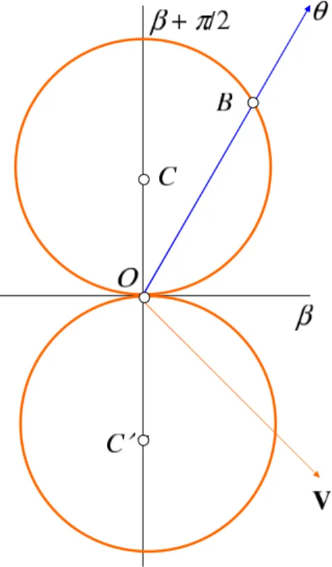
5 Wind waves velocities azimuth hodograph
From formulaλ˙K=6ksin(θ+θK)(see Eq. 21) one can see, that the wind waves velocities diagram is also a circle. We are going to call the wind waves velocities diagramazimuth hodographof the wind waves.
5.1 Motionless wind waves
The azimuth hodograph circle of the wind waves touches the straight lineθ=−θK,θ=−θK+π. Therefore at the direction θ=−θKthe wind waves velocity equals zero.
In the orthogonal direction θ=(π/2)sgn(K)−θK (see Eq. 21) the zero velocity troughs are located. We will call the waves with zero velocity asmotionlesswaves. In the motion-less wave’s troughs foam, driftweed and other minor material from the water surface is accumulated. Thereby the motion-less waves are marked on the water surface as motionmotion-less light stripes called “the Langmuir stripes”. The motionless waves are seen on the water surface air photographs at strong wind (Fig. 1). We do not consider in this paper the Langmuir circulations as it was made in the paper (Craik and Leibovich, 1976), though it should be noted, that our approach is more preferable, since we use both the water current and the wind currant and not just the surface stresses as in the paper (Craik and Leibovich, 1976).
If put aside all the damped neutral and non damped wind waves and leave only the motionless waves, the water sur-face will become crimped in the direction orthogonal to the Langmuir stripes. The amplitude of such a goffer dimin-ishes at damped waves and increases up to total destruction at non damped waves. The goffer of the neutral wind waves is frozen-in the other waves until the wind blows.
As a result of the wind waves dynamic interaction the mo-tionless Langmuir stripes are described here for the first time. The center of the wind waves velocities hodograph is sit-uated of the strait lineθ=(π/2)sgn(K)−θK at the distance
1
26K from the point of contact of the hodograph with the lineθ=−θK,θ=−θK+π(Fig. 3).
The axisθ=(π/2)sgn(K)−θK of the wind waves veloci-ties hodograph rotates at the parameterKchange (see the for-mulas (21), defining the trigonometric functions of the angle θK). That is why there is no wave velocity similarity theo-rem.
velocity for the given parameterK value. The vectorOA
in Fig. 3 equals the wind waves velocities at the direction θ(for the given parameterK value). The vectorV1equals the wind velocity. All the azimuths are counted out from the vectorV1on thez-plain. The velocity hodograph diameter directed along the maximal wind waves velocity6Kis called the main diameterof the hodograph.
5.2 σ-hodograph
Let us find the wind waves velocity along the directionθ=β. Let in the formula (18)θ=β and take into account formulas (16). Then
σ = √
Asin(β+γ )
1+d =
V1V0sinα
q
V12−2V1V0cosα+V02
. (22)
Here velocity σ≡λK(β)is the velocity of the zero length waves that is the velocity of the wave ripples in the direction θ=β.
σ-hodograph is the circle which main diameter equals toσ and is directed along the azimuthθ=β at 0≤α≤π and along the azimuthθ=β+π at(−π )<α<0. Theσ-hodograph cir-cle takes the form:
˙
λσ =σcos(θ−β), (0≤α≤π ). (23) Let us find the minimal value of the velocity6K with re-spect to parameterK using the formulas (21) and (16). It turns out as a result that the minimum is obtained at
K=Kσ = −C
B, (24)
and min
K |6K| =maxθ minK |˙λK| = |σ|. (25) This means that the minimal wind waves velocity with re-spect toKequals|σ|.
But the main property of the wind waves velocity of zero length is that the velocityσ does not depend of the growth rate1. That is why since the valueKσ corresponding to the main diameter of theσ-hodograph (see Eq. 24) belongs to a set of values of the parameterK, the main diameterσ of theσ-hodograph is a chord ofanyvelocity hodograph of the wind waves. Now it is possible to formulate the main the-orem of geometric dynamics of the non gravitational wind waves:
The locus of all the centers of the main diameters of the wind waves velocity hodographs is a strait line passing perpendicular to the vectorσ via its middle.
1In accordance with the formula (22) the parameterσis
calcu-lated after when the velocities of the air and water flowsV1andV0 and the angle between them have been obtained.
Fig. 3.Wind waves velocities azimuth hodograph.
The locus of all the main diameters ends of the wind waves velocity hodographs is a strait line passing perpendicular to the vector σ via their ends.
Consequence.
Since the vectorσ is oriented along or against the rayθ=β, perpendicular to the vectorσcenters line and the main diameters ends line are parallel to the axisθ=β±π/2 of the wavelengths diagram.
Therefore, the wavelengths diagram, the main σ -hodographs diameter and the two lines: the line of the centers of the main velocity hodographs diameters and the line of the ends of the same main diameters enter into the general skele-ton of the wind waves dynamics.
The physical meaning of the theorem and its consequence is in the fact that the mainσ-hodograph diameter can be mea-sured by the value and direction2.
6 Absolutely motionless waves, freak waves
Motionless wind waves in this approach appear in a natural way since the sine in the formula
˙
λK =6Ksin(θ+θK) (26)
always reduces to zero at the directionθ=−θK (see Eq. 21). There appears a question whether wind waves with zero ve-locity exist at any azimuth valueθ. To answer this question let us see at what values of theKparameter reduces to zero the coefficient6K(K)in the formula (26). Applying once again to the formulas (21) we can see that there are two such values. Their expressions after some simplifications take the form:
K=K0=
2δ(V −V0) δV +V0
(α=0), (27)
2The vectorσ direction is defined by the sign of the function
Kπ =
2δ(V +V0) δV −V0
(α= ±π ).
At these growth rate values the wind waves represent a dynamic barkhan-like water surface deformation. The height of the water barkhans diminishes if the values (27) are less than unity and increase up to overturning atK0>1 orKπ>1. IfK0=1 orKπ=1, the wind born water barkhan are neutral. The barkhan like waves are encountered in the vicinity of south-east Africa and more rearly along the Gulf Stream flow. In the case when the barkhan like wave’s amplitude increases quickly(K>1), the absolutely motionless wave is called freak wave, rogue wave, rabid-dog wave and so on. The waves like this sometimes sink ships. In the south-east Africa region the rogue waves appear on the Agulhas Current when the wind is directly oriented along the water current (α=0). This Agulhas Current and the Agulhas Retroflection can give rise to immense rogue waves that can threaten su-pertankers. For that reason, mariners who successfully nav-igated the Cape of Good Hope frequently breathed a sigh of relief. A very well known is the New Year’s Day wave, that struck the stationary Draupner oil platform in the North Sea on 1 January 1995. During this event, minor damage was in-flicted on the platform, confirming that the reading was valid. From that time it was concidered that once thought to be only legendary, they are now known to be anatural phenomeon, not rare, but rarely encountered. On the Gulf Stream in the region of the Bermuda Islands, the rogue waves appear and gain height of 18 meters. In 1912 in the Bermuda Islands re-gion a three masts sailing vessel was knocked out by a rogue waves of 30 m high. The next wave sank the vessel.
7 Wind waves express-forecast 7.1 (−2δ)-hodograph
Let us assume in the formula (20)K=−2δ. Then obtain the velocity hodograph of the wind waves
v(−2d)=Vcosθ (28)
The main hodograph diameter (28) is oriented along the wind vectorV. The radius of the velocity hodograph circle (28) equals half of the wind velocity. Since(−2δ)<1, the hodograph (28) (the wind velocity hodograph) belongs to the damped weaves set.
Despite the simplicity of the hodograph (28), it illustrates the main property of the considered waves: the wind waves propagate at many possible directions (in the considered case it is the direction(−π≤θ≤π )). The usual plane waves would propagate only in one direction (θ=0).
7.2 2-hodograph
Assume in the formula (20)K=2. Then obtain the velocity hodograph of wind waves
v2=V0cos(θ−α). (29)
The main hodograph diameter (29) is oriented along the velocity vector of the underwater currentV0. The radius of the velocity hodograph circle (29) equals 12V0. Since 2>1, the hodograph (29) (the underwater current velocity hodo-graph) belongs to the set of non damped waves.
Both hodographs (28) and (29) can be defined by means of measurements and simplest calculations of the angleβ. Indeed, let us choose on thezplane an arbitrary poleOand draw two vectors from it: vectorV of the air velocity and vectorV0 of the underwater current velocity. Consider the triangleOV V0. This triangle can always be plotted since its two sides(V andV0)and the angleαbetween them can be measured.
Remind now that the locus of the main diameters of the wind waves velocities is a straight line. Since the vectors
V andV0are the main diameters of some hodographs the whole line of the ends of the wind waves hodographs main diameters passes by the ends of the vectorsV andV0that is, the line of the wind waves hodographs main diameters ends contains the triangleOV V0base opposite to theOapex.
Now it is clear that the locus of the hodographs centers of the wind waves is the triangle’sOV V0centerline parallel to the baseV V0.
Therefore, one can conlude that the locuses of the centers of the wind waves velocities hodographs and the ends the same diameters are easily determined by means of wind and underwater current velocities measurements.
It is easily understood that the main diameter σ of the σ-hodograph is an oriented triangleOV V0 altitude passed from the apexO.
7.3 The main hodographs diameters orientation sectors The wind waves dynamics has one peculiarity. As we have just seen, the main diameterVof the hodograph (28) belongs to the region of non damped waves. The main diameterV0of the hodograph (29) belongs to the region of damped waves. What is the hodograph that is the boundary dividing the damped and the non damped waves? At first sight the answer is simple: the boundary is the hodographλ˙1=61sin(θ+θ1) (see Eq. 21) of neutral waves(K=1). Indeed at K<1 the wind waves damp and atK>1 do not damp right up till de-struction a cause of the wave amplitude growth.
So, if we move along the centers of the wind waves hodographs from the azimuth θ=β−π/2 to azimuth θ=β+π/2, the situation changes. Point is, that the hodo-graphK=±∞, that is, (by the Eq. 18), the hodograph
v∞= √
A
1+δsin(θ+γ ) (30)
Fig. 4.A freak wave.
Let us mark the center C of the hodograph (Eq. 30) (K=∞) on the centers line of wind waves velocities hodographs.
If we move along the indicated line of the centers from the pointC (K=∞)to the pointK=1 we will pass the cen-ters of the velocities hodographs of the non damped waves (1<K<∞). AtK=1 we get to the center of the velocities hodograph of neutral waves. At the further decrease of the parameterK, at 0<K<1 we move along the hodograph cen-ters of damped waves. AtK=+0 we obtain an internal res-onance of the growth rate of the waves with the turbulent re-sistance frequencyci=1 or in dimensional formc′i=κ. This will take place on the damped waves.
Note, that at K=2>1 the hodograph (29) of the water current velocity enters the velocities hodographs set of non damped waves. The main hodograph (29) diameter is lo-cated on the rayθ=α. That is why at 0≤α≤π the velocities hodographs centers of the wind waves atK→+0 go upward along the ray3θ=β+π/2.
Let us pass now from the pointC (K=−∞)to the point K=−0. We will again pass along the hodographs centers of the wind waves velocities but this time along the ve-locities hodographs centers we go downward along the ray θ=β−π/2.
Thus the orientation sectors of the main diameters hodographs of the damped waves at +0<K<1 and −∞<K<−0 are divided by the orientation sector of the main hodographs diameters of the damped waves velocities (1<K<∞). In this sense the damped waves at+0<K<1 and at−∞<K<−0 differ from each other and the waves at +0<K<1 we will callweakly dampedin contrast tostrongly dampedwaves at−∞<K<−0 (see Fig. 5).
3Motion downward along the rayθ=β−π/2 in this case is
im-possible since at 0≤α≤πthe azimuthθ=β−π/2<0
Fig. 5. Distribution of the sectors of the strongly- and weakly-damped waves
In the point of view of the Fig. 5 the destroying non-damped waves are weaker than the non-damped waves, since the orientation sector of the velocities hodographs of non damped waves occupy smaller part of the wave surface.
Let us take an arbitrary poleO on thez-plane. Draw via the poleOa counting out vectorV1of the azimuthsθ. Than via poleOdraw a skeletonθ=β,θ=β+πandθ=β±π/2 of the waves lengths diagram (Fig. 6).
Let us draw a vector σ the main diameter of the σ-hodograph from the pole O along the azimuth θ=β (0≤α≤π ). Along the azimuthθ=α from the poleO draw a vectorV0 of the velocity of the underwater current. Via the ends of the vectorsV andV0draw a straightP Q– line of the ends of the main hodographs diameters of the wind waves velocities (Fig. 6).
Draw a lineMN via the triangleOV V0centerline of the centers of the main hodographs diameters of the wind waves velocities.
Let us fix the parameterK , make for its value a waves lengths diagram and draw a tangentθ=−θK,θ=−θK+π to the velocities hodograph of the wind waves with the growth rateci=K−1.
Draw a rayθ=θK′ =(π/2)sgn(K)−θK via the poleO up to the centers lines and the ends of he main wind waves ve-locities diameters intersection.
As a result make a main diameter of the velocities hodo-graph of the wind waves with the given growth rate. The hodograph center is in the intersection point of the lineMN with the rayθ=θK′ . The main hodograph diameter end of the velocities is in the intersection point of the lineMNwith the same rayθ=θK′ (Fig. 6).
Knowing the rayθ=θK′ let us define the maximum wind waves velocity6K of the given growth rate and their length ℓK=OD(Fig. 6):
Fig. 6.The wind waves express forecast.
In the intersection point of the strait lineθ=β±π/2 with the velocities find the velocityσK of the waves of maximal length
σK=6Kcos(θK+β±π/2).
Having fixed some directionθ (Fig. 6), find the velocity
OAand the wave lengthOBin this direction.
The non gravitational wind waves have one more interest-ing property: the waves of the equal velocity value can have different wave lengths. The waves of equal wave length can have different velocities.
For example, in the direction θ=β, the wave velocity equalsσ, and the wave length equals zero. The waves sym-metric with respect to the axisθ=θK′ of the hodograph have the same velocity valueOE, but not the same wave length OF.
The neutral waves(K=1)of the equal velocity and dif-ferent wave length represent choppy sea. The problem of choppy sea has not been yet described analytically. Here this problem is solved with the use of a couple of circles.
The double lines on the Fig. 6 mark the Langmuir stripes that are evidently parallel to the main hodograph diameter 6Kof the wind waves velocities at the given value ofK. The lines LKB,B0O and others (Fig. 6) represent the troughs lines of the wind waves propagating with velocityλ˙K along the azimuthθ.
8 Conclusions
A common practice in both theoretical and practical hydro-dynamics is to consider sea waves as gravitational. Results presented in this work at least qualitatively coincide with both visual observations and with air-photography observa-tions, therefore assure us that the main sea and river waves have not the gravitational but turbulent nature: the initial re-lations (14) do not contain the accelerationg. These relations have a profound hydrodynamic nature – cluster and micro-heterogeneous liquid structure and as the consequence their turbulent resistance — the main wind waves stimulator, since in its absence (κ=κ1=0) it is impossible to formulate the ini-tial non disturbed adjacency current (2). It is quite natural, that though the approximately obtained dispersion relation (14), proves to be so informative. These relations not only explain all the main properties of the considered waves (vari-ety, crestedness, propagation direction, velocity, wave length, choppy sea etc.), but also reveal new – motionless – waves that are marked on the water surface by driftweed, foam as light Langmuir stripes, and thus are observed on the water surface in windy weather as real motionless waves. The value of turbulent resiatanceκ for air and water have to be measured experimentally. Recently, we obtained the value forκ in case of turbulent flow of water through a pipe (to be published). The value isκ=0.023 1/s. Using this value for both water and air turbulent resistance, and reasonable esti-mation for wind velocity (10 m/s), water velocity (1 m/s), and α=30◦one obtains from (19) estimation of the wavelength of the Langmuir waves approximately 21 m. More precise val-ues are subject of further experimental work.
Edited by: U. Harlander
Reviewed by: two anonymous referees
References
Birkhoff, G.: Hydrodynamics, Princeton, New Jersey, Princeton University Press, 1960.
Cherkesov, L. V.: Hydrodynamics of waves, Kiev: “Naukova Dumka”, 260 pp., 1980 (in Russian).
Craik, A. D. D. and Leibovich, S.: A rational model for Langmuir circulations, J. Fluid Mech., 73, 4001–426, 1976.
Gill, A. E.: Atmosphere-Ocean Dynamics, Academic Press, Lon-don Ltd., 1982.
Kochin, N. E., Kibel, I. A., and Roze, N. V.: Theoretical Hydrome-chanics, Interscience Publishers, John Wiley & Sons, 1964. Kondrat’ev, K. Ya., Nikanorov, A. M., Pantuhin, Ya. V., and
Za-volzhensky, M. V.: Ekman drift and other currents in unbounded regions, Doklady Akademii Nauk USSR, 310(5), 1070–1074, 1990.
Lamb, H.: Hydrodynamics, Cambridge, The Univ. Press, 1932. Monin, A. S.: Hydrodynamics of atmosphere, ocean and Earth
in-terior, St. Petersburg, Hydrometeoizdat, 524 pp., 1999.
Nekrasov, A. I.: Exact theory of steady waves on the heavy fluid sur-face, Collection of works, V I. Phys. Math. Ed., 358–439, 1961. Sajjadi, S. G., Thomas, N. H., and Hunt, J. C. R.: Wind-over-Wave Couplings: Perspectives and Prospects, Oxford University Press, USA, 384 pp., 1999.
Stocker, J. J.: Water Waves, Pure and Applied Mathematics, Vol. 9, The Mathematical Theory and Applications, Institute of Mathe-matical Sciences, New York University, USA, 291–314, 1957. Struminskii, V. V.: On the theory of Boltzmann kinetic equation,
RGD, Vol. 1, VI Int. Symp., N.Y., Akad. Press, 1969.
Titov, L. F.: Wind waves, Hydro. Meteo. Ed., 294 pp., 1969 (in Russian).