A NOVEL MULTICLASS SUPPORT VECTOR MACHINE ALGORITHM USING MEAN REVERSION AND COEFFICIENT OF VARIANCE

ISSN: 1549-3644

© 2013 Science Publications

doi:10.3844/jmssp.2013.208.218 Published Online 9 (3) 2013 (http://www.thescipub.com/jmss.toc)

Corresponding Author: Bhusana Premanode, Centre for Bio-inspired Technology, Imperial College London, United Kingdom

A NOVEL MULTICLASS SUPPORT

VECTOR MACHINE ALGORITHM USING

MEAN REVERSION AND COEFFICIENT OF VARIANCE

1

Bhusana Premanode,

2

Jumlong Vongprasert,

3

Nop Sopipan and

1

Christofer Toumazou

1_{Centre for Bio-inspired Technology, Imperial College London, United Kingdom} 2

Ubon Rachathani Rajabhat University, Ubon Ratchathani, Thailand

3_{Nakhon Ratchasima Rajabhat University, Nakhon Ratchasima, Thailand}

Received 2013-03-31, Revised 2013-07-20; Accepted 2013-07-31

ABSTRACT

Inaccuracy of a kernel function used in Support Vector Machine (SVM) can be found when simulated with nonlinear and stationary datasets. To minimise the error, we propose a new multiclass SVM model using mean reversion and coefficient of variance algorithm to partition and classify imbalance in datasets. By introducing a series of test statistic, simulations of the proposed algorithm outperformed the performance of the SVM model without using multiclass SVM model.

Keywords: Support Vector Machine, Multiclass, Mean Reversion, Coefficient of Variance

1. INTRODUCTION

1.1. Background

on Mean

Reversion

and

Coefficient of Variance

There are many definitions of mean reversion. In general, it is an asset model, which shows that the asset price tends to fall (or rise) after hitting a maximum (or minimum). The process of mean reversion is a log-normal diffusion, but the variance does not growing in proportion to the time interval (Pillay and O’Hare, 2011). The variance grows at the start and sometimes it stabilises at a certain value. The most basic mean reversion model is the (arithmetic) (Uhlenbeck and Ornstein, 1930). This model is a stochastic process with stationary, Gaussian and Markovian distribution and use to describe the velocity of a massive Brownian particle under the influence of friction. In the other approach, Zhao et al. (2011) introduced AR process where the value drifted to its mean in the long run. Currently, two main methodologies are used for measuring the mean reversion, i.e., (i) variance ratio and (ii) regression. Cochrane (1988) has used the variance ratio to measure the relative importance of the random walk component.

Poterba and Summers (1988) and Lo and Mackinlay (1988) compared the relative variability of returns over different time horizons using the variance ratio in discrete time series. Bali and Demirtas (2008) confirmed these reports by showing that in a ‘high variance’ scenario and using the mean reversion concept could cause negative drift. Using regression tests, Fama and French (1992) determined the correlation with currency asset returns, while Chen and Jeon (2000) measured its mean reversion behaviour and found that the returns were positively autocorrelated over shorter periods but negatively autocorrelated over longer periods. To measure imbalance in multiclass datasets, Cieslak and Chawla (2009) recommended to use Coefficient of Variance to solve the problem. Diebold (2004) also reported mean reversion using fractional unit-root analysis of real exchange rates under the gold standard. Diebold (2004) showed that the power of the test for mean reversion could be raised.

1.2. Background on Against-All and

One-Against-One Strategies

binary SVM classifiers, each of which separates one class from all the rest. The SVM is trained with all the training examples of a class with positive labels and all the others with negative lables; and (ii) the “One-Against-One”, which builds one SVM for each pair of classes (Chen et al., 2009). More complex decomposition methods employing Error Correcting Output Codes (ECOC) have been introduced (Dietterich and Bakiri, 1995; Allwein et al., 2005). Hsu and Lin (2002) compared several multiclass SVM methods. The conclusion from their works is that “One-Against-One” is more practical, because the training process is quicker. Rifkin and Klautau (2004) disagreed with Allwein et al. (2005) that “One-Against-One” and other ECOC were more accurate than the “One-Against-All” strategy, arguing that the “One-Against-All” strategy war as accurate as any other approach by assuming that the SVMs are well tuned. Rifkin and Klautau (2004) concluded that a simple scheme such that One-Against-All and One-Against-One was preferable to a highly complex ECOC methods.

1.3. Background on the EMD Algorithm

The analysis of nonlinear and nonstationary data is important in many applications such as bioinformatics (Shi et al., 2008; Huang et al., 1996), signal processing (Huang et al., 1998; Huang and Attoh-Okine, 2005; Huang and Shen, 2005), geophysics (Wang et al., 1990; Datig and Shlurmann, 2004) and finance (Huang and Attoh-Okine, 2005; Guhathakurta et al., 2008). Huang et al. (1996) formulated an a posteriori algorithm with adaptive control over a separate data structure, which was later termed the Hilbert-Huang Transform (HHT) (Huang et al., 1998). The HHT overcomes the limitations of the Hilbert transform, which is only suitable for a narrow band-pass signal. The key element of the HHT algorithm is the EMD, in which any complicated dataset can be decomposed into a finite and often small number of Intrinsic Mode Functions (IMFs) that allow a well-behaved Hilbert transform. Since this decomposition is based on the local characteristic time scale of the data, it is applicable to nonlinear and nonstationary processes (Huang and Attoh-Okine, 2005). In signal processing, high-frequency noises from input data are considered simple intrinsic mode oscillations (Huang and Attoh-Okine, 2005). The EMD uses a sifting process and curve spline technique to decompose a signal into a new oscillatory signal termed the IMF. After a number of decomposition iterations, the

characteristics of the IMF must meet two conditions. First, in the entire dataset the number of extrema (maxima plus minima) and number of zero crossings must either be the same or differ by at most one. Second, at any point the mean values of the envelopes defined by the local maxima and the local minima must be zero (Huang and Shen, 2005). The EMD algorithm, which is fundamental to the HHT, can thus reduce high-frequency noise from input data, such as noise from retail trades on a stock exchange.

1.4. Objective

This study presents a novel multiclass SVM model using mean reversion and coefficient of variance algorithm to partition and classify the datasets; and then introduce SVM to measure their performance. For verification, we compared to the multiclass SVM model with another SVM model that was without mean reversion and coefficient of variance algorithm.

2. MATERIALS AND METHODS

2.1. SVM Model

There are several methods used for data classification, one of them being SVM. Let x be a vector in a vector space. A boundary hyperplane is expressed as one of the hyperplanes:

T

w x+ =b 0 (1)

Where:

w = A weight coefficient vector and

b = A bias term. The distance between training vectors xi = The boundary, called margin, is expressed as

follows:

T i w x b

w +

(2)

Since the hyperplanes expressed by Equation 1 where w and b are multiplied by a common constant are identical, we introduce a restriction to this expression, as follows Equation 3:

T i

min w x+ =b 1 (3)

reduced to maximisation of 2 T

1 1

w w

w = . As a result, the

underlying optimisation is formalised as Equation 4:

T

Minimize w w (4)

subject to yi (wTx+b)≥1.

where, yi is 1 if xi belongs to one set and yi is-1if xi

belongs to the other set. If the boundary classifies the vectors correctly, then yi (wTx+b)≥0, of which it is

identical to the margin.

This conditional optimisation is achieved by Lagrange’s method of indeterminate coefficient. Define a function:

(

)

T

(

T

)

i i i

i 1

L w, b, w w y w x b 1

2

 

α = −

∑

α _ + − _ (5)

where, αi ≥0 are the indeterminate coefficients. If w and

b take the optimal value, the partial derivatives are zero:

i i i i i

i i

L L

w y x , y

w b

∂ _{= − α} ∂ _{= − α}

∂

∑

∂

∑

(6)

By setting the derivatives of Equation 6 to zero, we obtain:

i i i i

w=

∑

αy x (7)

i i i

y 0 α =

∑

(8)

Rewriting Equation 5, we obtain:

(

)

T T

i i i i i i i

i i i

1

L w, b, w w y w x b y ,

2

α = −

∑

α −

∑

α +

∑

α (9)

Substituting Equations 7-9, we obtain Equation 10:

(

i

)

i i i T j j j

i j

T

i i j j j i

i j i

T

i j i j i j i

i j i

1

L w, b, y x y x

2

y y x

1

y y x x 2

 

 

α =  α   α 

   

 

− α  α  + α

 

= α α + α

∑

∑

∑

∑

∑

∑∑

∑

(10)

The contribution of the second term of Equation 5 should be minimised versus L should be maximised

subject to α. Consequently, the optimisation is reduced to a quadratic programming problem as follows:

T

i j i j i j i

i j i

i i i

i 1

Maximize y y x x 2

subject to y 0, 0

− α α + α

α = α ≥

∑∑

∑

∑

(11)

Let Φ be a transformation to a higher dimensional space. The transformed space should satisfy that the distance is defined in the transformed space and the distance has a relationship to the distance in the original space. The kernel function K(x,x’) is introduced for satisfying the above conditions. The kernel function satisfies:

(

)

( ) ( )

T

K x, x′ = Φ x Φ x′ (12)

The above Equation 12 indicates that the kernel function is equivalent to the distance between x and x’ measured in the higher dimensional space transformed by Φ. If we measure the margin by the kernel function and perform the optimisation, a nonlinear boundary is obtained. Note that the boundary in the transformed space is obtained as:

( )

T

w Φ x + =b 0 (13)

Substituting Equation 7 into the above Equation 13 while replacing x with Φ(x), we obtain:

( )

T

( )

(

)

i i i i i i

i i

y x x b y K x , x b 0

α Φ Φ + = α + =

∑

∑

(14)

The optimisation function of Equation 11 in the transformed space is also obtained by substituting

T i i

x x with K(xi,xj). These results mean that all the

calculation can be achieved by using K(xi,xj) only and we

do not need to know what Φ or the transformed space actually is.

A sufficient condition for satisfying Equation 14 is that K(xi,xj) is positive definite. Several examples of

such kernel functions are known, as follows: (Laplacian kernel function) Equation 15:

(

)

(

)

2.2. Data Classification Using Mean Reversion

and Coefficient of Variance Algorithm

We present a novel multiclass model for use with the SVM family using mean reversion and coefficient of variance algorithm to partition and classify the time horizon (span) of multiclass datasets, respectively. In practice, the typical curve of exchange rates tends to shift towards the mean, so the point of reversal can be used to determine changes in its direction, i.e., from up to down and vice versa. The datasets are then partitioned at the reversal point using the mean reversion algorithm, which later explained, as a decision tool. The standard deviations of a nonstationary datasets are not the same, so we measure the datasets between each reversal points and input them into a SVM model. The procedure for using mean reversion and coefficient of variance algorithm are as follows:

• Compute the mean µn (t) of random variables Xn (t)

• Compute the variance Vn (t) of Vn (t)

• After normalising each Vn (t) using µn (t), we obtain

n n V (t)

(t) µ

• In an upward scenario where V1(t)<V2(t),..,n or a

downward scenario where

• if 2 1

2 1

V (t) V (t) (t)< (t)

µ µ or 22 11

V (t) V (t) (t)> (t)

µ µ , mark the intercept point on the x-axis and denote it as M1, i.e., the

value is Xm (t) where r =1,2,..,c and c is the last class

using coefficient of variance equation (cv=σ µ where CV is coefficient of variance) or

• if n 1 n

n 1 n

V (t) V (t) (t) (t) −

− =

µ µ , do not use the intercept point on the x-axis

• Repeat 4) and stop when n n V (t)

(t)

µ is the last data point (n). Next, plot M2,…,Mn

• Compute CV for the data Xm (t) in blocks of M1,

M2,..,Mn where n-1 is the number of partitions/blocks

The original datasets Xn (t) was classified in different

classes of coefficient of varaince and termed to CV class. The next step aims to simulate Xn (t) individually using

the SVM model for each CV group. As a result, these multiple sets of kernel parameters in each SVM simulation are created; we then integrate all the blocks partitioned by the CV.

2.3. Cross Validation Methods

Schneider and Moore (1997) classified model evaluation into many methods, e.g., judging the model quality based on the residuals, black box model selection and validation. According to their reports, cross-validation is a model evaluation method that separates training and test data, which uses the test data to test the performance after the training data were computed by a statistical model. Cross-validation uses the following three main methods.

2.3.1. Holdout

The Holdout method is the simplest type of cross-validation. The datasets is separated into two sets: the training set and the test set. The estimation model fits the training set only and leaves the test data blind. The performance of the Holdout method can be quantified using a variety of test statistic, i.e., MSE, MAE, MAPE, R2, AIC and BIC. This method is usually preferable to the residual method and it does take that much no longer to compute. However, its evaluation can have a high variance, which may depend greatly on how the training and test data are divided. In this study, we select and divide datasets using different ratios of the training data and test data, i.e., 30:70, 50:50 and 70:30, respectively.

2.3.2. K-Fold

K-fold was proposed to improve the Holdout method. The K-fold method divides the entire datasets into k subsets and uses the Holdout method k times. In each subset, the training data are computed using the model and tested with the test data. Thus, the average error is computed across all k trials. The advantage of this method is that it is less important how the data is divided. Every data point is used in the test set exactly once and in a training set k-1 times. The variance of the estimate is reduced to k is increased. The disadvantage of this method is that the training algorithm has to be rerun from scratch k times, which means it requires k times as many computation to make an evaluation. A variant of this method is to randomly divided the data into a test and training set k different times.

2.3.3. Leave-One-Out

the remaining data are used for reference. The advantage is that the accuracy of the outcome but this is traded-off by the massive computational power requirements when handling large input datasets. Moreover, this method was designed only for model evaluation or in-sample forecasting so it is rather difficult to apply this method to out-of-sample forecasting.

2.4. The OAO and OAA Strategies

In general, the multiclass SVM is an ongoing research issue and it can be fundamentally classified using two different strategies: (i) OAA consists of building one SVM per class and trains it while the rest of the training data remains as the other class so-called ‘All’. The method of building the ‘One’ class is flexible depending upon the structure of datasets and (ii) OAO is similar to the OAA strategy except the ‘All’ class is individually partitioned into subclasses. The discrimination of OAA strategy between an information class and all others often leads to the estimation of complex discriminant functions (Schneider and Moore, 1997). In brief, the OAO decomposes the original problem into a set of small problems of two information classes with n(n-1)/2 binary SVMs. In this study, we have selected mean reversion and coefficient of vraince algorithm for selecting the training data.

3. RESULTS

The simulations were conducted on a personal computer with clock frequency at 2.50GHz, Intel® core(TM) i5-3210 M CPU and 8 GB of RAM. All the SVMs were trained with R programming software (Kim and Oh, 2012). We use all kernel functions i.e., Gaussian, polynomial, linear, Laplace, Bessel and ANOVA RBF; then, select the best performance out of those functions.

With respect to Materails and Methods, we introduced theoretical considerations related to the SVM model and its background in supervised learning and its structure risk minimisation. We also selected the Holdout model, which is part of the model evaluation used to segregate training and test datasets, before partitioning them using the mean reversion and coefficient of variance algorithm. This technique is novel and it is used to construct a multiclass for the SVM family.

3.1. Simulation Procedure

We describe the simulation procedure used by the multiclass SVM model, as shown in Fig. 1. The systematic order of the workflow is as follows:

• Retrieve 2322 datasets, EUR-USD exchange rates from Bloomberg terminal from 2001 to 2011 • Demonstrating in Fig. 1, we use the Holdout method

to separate the datasets into the training and test data. After separation, each group has a ratio of 30:70, 50:50 and 70:30. The 30% of the datasets are used as out-of-sample forecasting

• At the reversal point of the curves resulted from the mean reversion technique described in 2.2, we use CV to classify each group of dependent variables and yields a number of sub-groups

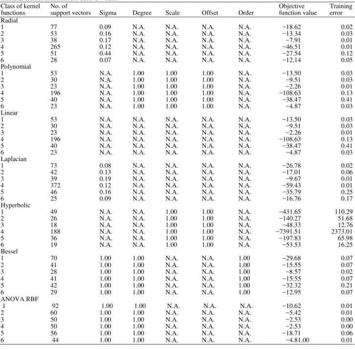
• From (3) for each sub-group we simulate the multiclass SVM model using the R programming software (Kim and Oh, 2012). This fits the multiclass kernel functions and parameters for each subgroup. During this stage, we obtain many kernel parameters for each group partitioned, as shown in Table 1

• Integrate all of the results from (4) in the time series domain. Finally, we produce a new classified datasets. • Quantify the performance of the multiclass SVM

model using a variety of test statistic, i.e., MSE, MAE, MAPE, R2, AIC, BIC and Accuracy counts which measures upward and downward movements of each local data point of the newly simulated datasets • Robustness test of the Multiclass SVM model with

OAA and OAO strategies: From (3) and Table 1, we assign the first CV class to ‘One’ and the remaining classes to ‘All’ as per the OAA strategy. Additionally, we select the second CV class and assign to ‘One’ and the remaining classes to ‘All’ and so on. Alternatively, we introduce OAO strategy; thus, the pairing of multiclass is as follows: a) Class 1 and Class 2, Class 1 and Class 3,…,

Class 1 and n where n is the last Class

b) Class 2 and Class 3, Class 2 and Class 4,…,Class 2 and Class n; until the final when c) Class n-1 and Class n

• For the One-Against-All strategy, we compare simulation results of the data points, which are located in the correct classes with the results from (5); and then analyse the percentage of error. For the One-Against-One strategy, use the outcomes from each paring to vote for the best performance in each class

3.2. Simulation Results

different ratios, i.e., 30:70, 50:50 and 70:30. We introduced the mean reversion and coefficient of variance algorithm to partition and classify the training data, respectively. We intended to leave the test data to be used as reference in order to compare with the predicted outcome from the SVM simulation. As a result, 48 blocks/partitions were separated into six CV classes, at which are shown in Table 1. We then grouped each CV class and simulated them with the SVM classification model using R Programming scripts (Kim and Oh, 2012). The simulated are shown in Table 2-6.

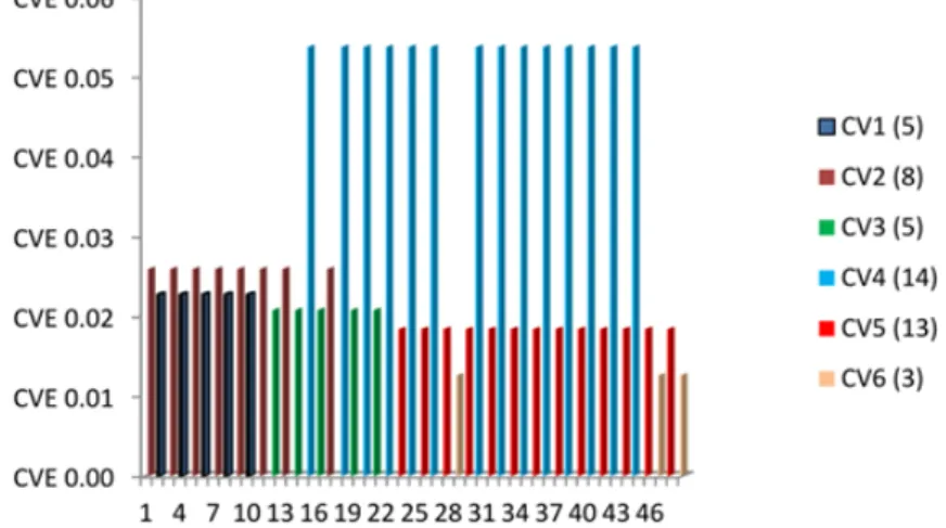
Table 1 was used to plot a graph and Fig. 2 illustrates

the distribution of the six CV classes where the x-axis represented 50 blocks/partitions and the y-axis represented the CV values of the different classes. The figures in brackets show the number of data points per CV class and they were re-displayed in Table 4. Each block/partition contained different numbers of data points, depending on the change in the curve direction, i.e., upward to downward or vice versa.

At this point, we had classified datasets into multiclass. The next step was to run simulations of the SVM models. The results of those simulations are in Table 3.

We fitted the kernel distribution functions and their parameters. The outcomes shown in Table 2

using different sets of kernel functions, i.e., radial, polynomial, linear, Laplacian, hyperbolic, Bessel and ANOVA RBF, were different. Moreover, the number of support vectors, parameters and training error were presented in Fig. 2. Definitions of the parameters given in the Table 2 are as follows:

• Sigma: the inverse kernel width used by the Radial, Gaussian, Laplacian, Bessel and ANOVA RBF kernel functions

• Degree: the degree of the polynomial, Bessel or ANOVA RBF kernel functions, i.e., a positive integer

• Scale: the scaling parameter of the polynomial and tangent kernel functions is a convenient way of • normalising patterns without any need to modify the

data itself

• Offset: the offset used in polynomial or hyperbolic tangent kernel functions

• Order: the order of the Bessel function

Next, we used the test statistic, i.e., MSE, MAE and MAPE, to measure the performance of each kernel function in all CV classes of the datasets. The results given in Table 3 show that the Laplacian kernel functions performed the best. Having successfully simulated the SVM with

Laplacian kernel functions and parameters, in conclusion there were six CV classes in 48 blocks/partitions and each block had a different number of data points.

Table 4 shows the CV classes including the

Laplacian kernel functions and parameters. At this stage, we completed simulations required for building up the training data.

Referring to the SVM model for classification, we simulated the test data, which came from the ratio of training and test data at 70:30, by using the trained Laplacian kernel functions and their parameters. The simulation results of the three datasets shown in Fig. 3, at which the x-axis represented the number of data points used for classification and the y-axis represented the EUR-USD. Finally, the results demonstrated that the graph of the multiclass SVM model in black solid line agreed with the graph of the original datasets in dotted blue line, whereas the graph of SVM model only was deviated from those two graphs. To ease for presentation, the x-axis represented the test data ranking between 2001st to 2049th of the original datasets.

To verify the performance of the multiclass using the mean reversion and coefficient of variance algorithm, we plotted three graphs, which showed the simulation results for the multiclass SVM model and the SVM without multiclass algorithm (SVM model only). The two graphs of the SVMs after simulations with and without multiclass were significantly different, as shown in

Table 5. Using the Laplacian kernel function and a

training:test data ratio of 70:30. For example, we compared the Accuracy count which was 79.88%, whereas the SVM model without the multiclass algorithm measured by Accuracy count of 73.21%. Finally, we measured the performance of the multiclass SVM model comparing with the SVM model only by using the test statistic, i.e., MSE, MAE, MAPE, R2, AIC and BIC. The results in Table 5. showed that the proposed model outperformed the performance of the simulation from the SVM model only.

3.3. Robustness Test

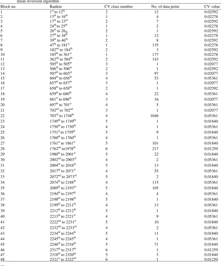
Table 1. Classification of the CV class ranking for each block, the CV and their related values and the number of blocks created by mean reversion algorithm

Block no. Rankin CV class number No. of data point CV value

1 1st to 12th 2 12 0.02592

2 13th to 16th 1 4 0.02278

3 17th to 23rd 2 7 0.02592

4 24th _{to 25}th _{1 2 0.02278}

5 26th to 26th 2 1 0.02592

6 27th to 38th 1 12 0.02278

7 39th to 46th 2 8 0.02592

8 47th _{to 181}st _{1 135 0.02278}

9 182nd to 184th 2 3 0.02592

10 185th _{to 361}st _{1 177 0.02278}

11 362nd to 504th 2 143 0.02592

12 505th to 505th 3 1 0.02077

13 506th to 506th 2 1 0.02592

14 507th to 603rd 3 97 0.02077

15 604th to 656th 4 53 0.05361

16 657th to 657th 3 1 0.02077

17 658th to 658th 2 1 0.02592

18 659th to 680th 4 22 0.05361

19 681st to 696th 3 16 0.02077

20 697th to 701st 4 5 0.05361

21 702nd to 702nd 3 1 0.02077

22 703rd to 1748th 4 1046 0.05361

23 1749th to 1749th 5 1 0.01840

24 1750th to 1750th 4 1 0.05361

25 1751st to 1759th 5 9 0.01840

26 1760th to 1760th 4 1 0.05361

27 1761st to 1861st 5 101 0.01840

28 1762nd to1978th 6 217 0.01259

29 1980th to 2001st 5 22 0.01840

30 2002nd to 2003rd 4 2 0.05361

31 2004th to 2016th 5 13 0.01840

32 2017th _{to 2071}st _{4 55 0.05361}

33 2072nd to 2073rd 5 2 0.01840

34 2074th to 2188th 4 115 0.05361

35 2089th to 2193rd 5 105 0.01840

36 2194th to 2197th 4 4 0.05361

37 2198th _{to 2198}th _{5 1 0.01840}

38 2199th to 2211th 4 13 0.05361

39 2212th to 2212th 5 1 0.01840

40 2213th to 2221st 4 9 0.05361

41 2222nd to 2231st 5 10 0.01840

42 2232nd to 2233rd 4 2 0.05361

43 2234th to 2244th 5 11 0.01840

44 2245th to 2245th 4 1 0.05361

45 2246th to 2316th 5 71 0.01840

46 2317th to 2317th 6 1 0.01259

47 2318th to 2320th 5 3 0.01840

Table 2. Kernel functions for each CV class

Class of kernel No. of Objective Training

functions support vectors Sigma Degree Scale Offset Order function value error Radial

1 77 0.09 N.A. N.A. N.A. N.A. −18.62 0.02

2 53 0.16 N.A. N.A. N.A. N.A. −13.34 0.03

3 38 0.17 N.A. N.A. N.A. N.A. −7.91 0.01

4 265 0.12 N.A. N.A. N.A. N.A. −46.51 0.01

5 51 0.44 N.A. N.A. N.A. N.A. −27.54 0.12

6 28 0.07 N.A. N.A. N.A. N.A. −12.14 0.05

Polynomial

1 53 N.A. 1.00 1.00 1.00 N.A. −13.50 0.03

2 30 N.A. 1.00 1.00 1.00 N.A. −9.51 0.03

3 23 N.A. 1.00 1.00 1.00 N.A. −2.26 0.01

4 196 N.A. 1.00 1.00 1.00 N.A. −108.63 0.13

5 40 N.A. 1.00 1.00 1.00 N.A. −38.47 0.41

6 23 N.A. 1.00 1.00 1.00 N.A. −4.87 0.03

Linear

1 53 N.A. N.A. N.A. N.A. N.A. −13.50 0.03

2 30 N.A. N.A. N.A. N.A. N.A. −9.51 0.03

3 23 N.A. N.A. N.A. N.A. N.A. −2.26 0.01

4 196 N.A. N.A. N.A. N.A. N.A. −108.63 0.13

5 40 N.A. N.A. N.A. N.A. N.A. −38.47 0.41

6 23 N.A. N.A. N.A. N.A. N.A. −4.87 0.03

Laplacian

1 73 0.08 N.A. N.A. N.A. N.A. −26.78 0.02

2 42 0.13 N.A. N.A. N.A. N.A. −17.01 0.06

3 39 0.19 N.A. N.A. N.A. N.A. −9.67 0.01

4 372 0.12 N.A. N.A. N.A. N.A. −59.43 0.01

5 46 0.16 N.A. N.A. N.A. N.A. −35.79 0.25

6 25 0.09 N.A. N.A. N.A. N.A. −16.76 0.17

Hyperbolic

1 49 N.A. N.A. 1.00 1.00 N.A. −431.65 110.29

2 26 N.A. N.A. 1.00 1.00 N.A. −140.27 51.68

3 18 N.A. N.A. 1.00 1.00 N.A. −48.33 12.76

4 188 N.A. N.A. 1.00 1.00 N.A. −7391.51 2373.01

5 36 N.A. N.A. 1.00 1.00 N.A. −197.83 65.98

6 19 N.A. N.A. 1.00 1.00 N.A. −53.53 16.25

Bessel

1 70 1.00 1.00 N.A. N.A. 1.00 −29.68 0.07

2 41 1.00 1.00 N.A. N.A. 1.00 −15.55 0.07

3 28 1.00 1.00 N.A. N.A. 1.00 −8.57 0.02

4 41 1.00 1.00 N.A. N.A. 1.00 −15.55 0.07

5 42 1.00 1.00 N.A. N.A. 1.00 −32.32 0.21

6 29 1.00 1.00 N.A. N.A. 1.00 −12.95 0.07

ANOVA RBF

1 92 1.00 1.00 N.A. N.A. N.A. −10.62 0.01

2 60 1.00 1.00 N.A. N.A. N.A. −5.42 0.01

3 50 1.00 1.00 N.A. N.A. N.A. −2.53 0.00

4 50 1.00 1.00 N.A. N.A. N.A. −2.53 0.00

5 56 1.00 1.00 N.A. N.A. N.A. −18.71 0.06

6 44 1.00 1.00 N.A. N.A. N.A. −4.81.00 0.01

Table 3. Performance evaluation for all kernel functions

Kernel function MSE MAE MAPE

Radial 3.84E-05 0.0048831 0.375369

Polynomial 0.000520 0.0159646 1.212167

Linear 0.000520 0.0159676 1.212442

Laplacian 3.24E-05 0.0046254 0.360253

Hyperbolic 6.192284 1.5028091 113.5211

Bessel 0.000483 0.0128695 0.985140

Table 4. Details of the number of blocks per CV class, the parameters of the CV class and its value

Class Blocks Parameter of Laplacian kernel function CV

1 5 F(w,x) = wT exp(-0.880257537388077 || x-x’||)+b 0.02278 2 8 F(w, x) = wT exp(-0.126109678105003 || x-x’||)+b 0.02592 3 5 F(w, x) = wT exp(-0.1872440577155 || x-x’||)+b 0.02077 4 14 F(w, x) = wT exp(-0.120770384940063 || x-x’||)+b 0.05361 5 13 F(w, x) = wT _{exp(-0.156375637970856 || x-x’||)+b 0.01840}

6 3 F(w, x) = wT exp(-0.880257537388077 || x-x’||)+b 0.01259

Table 5. Simulation results using the multiclass SVM model compared with simulations using the SVM model without multiclass (SVM only), using the original dataset was the reference

Test statistic SVM model only Multiclass SVM model

Accuracy counts

30:70 70.2600000 78.210000

50:50 70.6000000 78.9200000

70:30 73.2100000 79.8800000

MSE 0.0001429 3.242E-05

MAE 0.0098611 0.0046254

MAPE 0.6946638 0.3602532

R2 0.9827000 0.9992000

AIC −4213.8360000 −5209.8460000

BIC −4200.2000000 −5196.2180000

Fig. 1. Diagram showing the multiclass SVM model with robustness tests using OAA and OAO strategies

Fig. 3. Performance of the multiclass SVM model compared with the original dataset where the plot on the x-axis represents the test data at 2001st to 2049th of the entire datasets

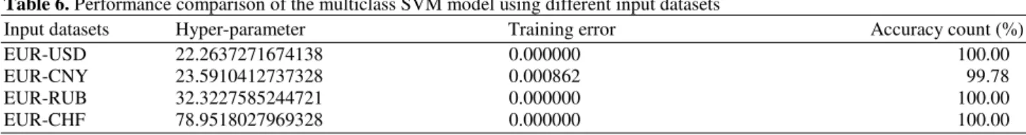
Table 6. Performance comparison of the multiclass SVM model using different input datasets

Input datasets Hyper-parameter Training error Accuracy count (%)

EUR-USD 22.2637271674138 0.000000 100.00

EUR-CNY 23.5910412737328 0.000862 99.78

EUR-RUB 32.3227585244721 0.000000 100.00

EUR-CHF 78.9518027969328 0.000000 100.00

In the parameter selection of the SVM simulation software, we selected Laplacian kernel function and compared the results simulations of the OAA and OAO strategies. Table 6 presented performance comparison of the multiclass SVM models using the different input datasets. The Accuracy count for the OAA and OAO strategies reached to 100% for every single simulated input data except EUR-CNY yielded 99.78% and the training errors of each simulation were similar.

4. DISCUSSION

The mechanism of mean reversion and coefficient of variance algorithm started by classifying each datasets with its mean, giving two separated groups, termed to ‘mean1+’ and ‘mean1– ‘; and continue to divide each

mean1+’ and ‘mean1–’ until the minimum and maximum

values of the datasets located in both ends. Therefore, we may obtain ‘mean2+’ and ‘mean2–’ inasmuch as ‘mean3+’

and ‘mean3–’ and so on. In this study, we optimise the

classification process; and have found six possible CV classes. The future work will be in the area of optimization of kernel functions in the frequency domain.

5. CONCLUSION

The multiclass algorithm for SVM model consists of mean reversion and coefficient of variance algorithm using for partition and classification nonlinear nonstationary datasets yields a significant outcome, compared with the conventional SVM model without multiclass algorithm. To verify the robustness of the proposed algorithm, the OAA and OAO strategies were introduced. By using a variety of test statistic, the simulation results using different inputs from many exchange rates i.e., EUR-USD, EUR-CNY, EUR-RUB and EUR-CHF confirmed that the proposed multiclass algorithm outperformed significantly the simulations of the conventional SVM model.

6. ACKNOWLEDGMENT

Jantratornkul and Wong Fan Voon, who read, edited and provided helpful suggestions.

7. REFERENCES

Allwein, E.L., R.E. Schapire and Y. Singer, 2000. Reducing multiclass to binary: A unifying approach for margin classifiers. J. Mach. Learn. Res., 1: 113-141. DOI: 10.1162/15324430152733133

Bali, T.G. and K.O. Demitras, 2008. Testing mean reversion in stock market volatility. J. Futures Markets, 28: 1-33.

Chen, J., C. Wang and R. Wang, 2009. Adaptive binary tree for fast SVM multiclass classification. Neurocomputing, 72: 3370-3375. DOI: 10.1016/j.neucom.2009.03.013

Chen, S.N. and K. Jeon, 2000. Mean reversion behavior of the returns on currency assets. Int. Rev. Econ. Finance, 7: 185-200. DOI: 10.1016/S1059-0560(98)90039-9 Cieslak, D.A. and N.V. Chawla, 2009. A framework for

monitoring classifiers’ performance: When and why failure occurs? Knowl. Inform. Syst., 18: 83-109. DOI: 10.1007/s10115-008-0139-1

Cochrane, J.H., 1988. How big is the random walk in GNP. J. Political Econ., 96: 893-920. DOI: 10.1086/261569

Datig, M. and T. Schlurmann, 2004. Performance and limitations of the Hilbert-Huang Transformation (HHT) with an application to irregular water waves.

Ocean Eng., 31: 1783-1834. DOI:

10.1016/j.oceaneng.2004.03.007

Diebold, F.X., 2004. The nobel memorial prize for robert f. engle. Scandinavian J. Econ., 106: 165-185. Dietterich, T.G. and G. Bakiri, 1995. Solving Multiclass

Learning Problems via Error-Correcting Output Codes. J. Arti Intell. Res., 2: 263-286. DOI: 10.1613/jair.105

Fama, E.F. and K.R. French, 1992. The cross-section of expected stock returns. J. Finance, 47: 427-465. DOI: 10.2307/2329112

Guhathakurta, K., I. Mukherjee and A. Roy, 2008. Empirical mode decomposition analysis of two different financial time series and their comparison. Chaos. Solut. Fractals, 37: 1214-1227. DOI: 10.1016/j.chaos.2006.10.065

Hsu, C.W. and C.J. Lin, 2002. A comparison of methods for multiclass support vector machines. IEEE Trans. Neural Netw., 13: 415-425. DOI:10.1109/72.991427 Huang, N.E. and N.O. Attoh-Okine, 2005. The Hilbert

Transform in Engineering. 1st Edn., CRC Press, ISBN-10: 0849334225, pp: 328.

Huang, N.E., Z. Shen and S.R. Long,M.C. Wu and H.H. Shih et al., 1998. The empirical mode decomposition and the hilbert spectrum for nonlinear and non-stationary time series analysis. Proc. R Soc. Lond. A., 454: 903-995.DOI: 10.1098/rspa.1998.0193

Huang, N.N.E. and S.S.P. Shen, 2005. Hilbert-Huang Transform and Its Applications. 1st Edn., World Scientific Publishing, Hackensack, ISBN-10: 9812563768, pp: 311.

Huang, W., Z. Shen, N.E. Huang and Y.C. Fung, 1996. Nonlinear indicial response of complex nonstationary oscillations as pulmonary hypertension responding to step hypoxia. Proc. Nat. Acad. Sci., 96: 1834-1839. DOI: 10.1073/pnas.96.5.1834

Kim, D. and H.S. Oh, 2012. EMD: Empirical Mode Decomposition and Hilbert Spectral Analysis. Lo, A.W and A.C. MacKinlay, 1988. Stock market

prices do not follow random walks: Evidence from a simple specification test. Rev. Financ. Stud., 1: 41-66. DOI: 10.1093/rfs/1.1.41

Pillay, E. and J.G. O’Hare, 2011. FFT based option pricing under a mean reverting process with stochastic volatility and jumps. J. Comput. Applied Math., 12: 3378-3384. DOI: 10.1016/j.cam.2010.10.024

Poterba, J.M. and L.H. Summers, 1988. Mean reversion in stock prices: Evidence and implications. J. Financ. Econ., 22: 27-59. DOI: 10.1016/0304-405X(88)90021-9

Rifkin, R. and A. Klautau, 2004. In defense of one-vs-all classification. J. Mach. Learn. Res., 5: 101-141. Schneider, J. and A. Moore, 1997. A Locally Weighted

Learning Tutorial using Vizier 1.0. Carnegie Mellon University.

Shi, F., Q.J. Chen and N.N. Li, 2008. Hilbert Huang transform for predicting proteins subcellular location. J. Biomed. Sci. Eng., 1: 59-63. DOI: 10.4236/jbise.2008.11009

Uhlenbeck, G.E. and L.S. Ornstein, 1930. On the Theory of the Brownian Motion. Phy. Rev., 36: 823-841. DOI: 10.1103/PhysRev.36.823

Wang, L., C. Koblinsky, S. Howden and N.E. Huang, 1990. Interannual variability in the south china sea from expendable bathythermograph data. J. Geophys. Res., 104: 509-523. DOI: 10.1029/1999JC900199