www.atmos-chem-phys.net/15/7247/2015/ doi:10.5194/acp-15-7247-2015
© Author(s) 2015. CC Attribution 3.0 License.
Low hygroscopic scattering enhancement of boreal aerosol and the
implications for a columnar optical closure study
P. Zieger1, P. P. Aalto2, V. Aaltonen3, M. Äijälä2, J. Backman2,a, J. Hong2, M. Komppula4, R. Krejci1,2, M. Laborde5,6, J. Lampilahti2, G. de Leeuw2,3, A. Pfüller4, B. Rosati7, M. Tesche1,b, P. Tunved1, R. Väänänen2, and T. Petäjä2
1Stockholm University, Department of Environmental Science and Analytical Chemistry & Bolin Centre for Climate Research, Stockholm, Sweden
2University of Helsinki, Department of Physics, Helsinki, Finland
3Finnish Meteorological Institute, Climate Research Unit, Helsinki, Finland
4Finnish Meteorological Institute, Atmospheric Research Centre of Eastern Finland, Kuopio, Finland 5AerosolConsultingML GmbH, Lausanne, Switzerland
6Ecotech Pty Ltd., Melbourne, Australia
7Paul Scherrer Institute, Laboratory of Atmospheric Chemistry, Villigen, Switzerland
anow at: Finnish Meteorological Institute, Atmospheric Composition Research, Helsinki, Finland bnow at: University of Hertfordshire, School of Physics, Astronomy and Mathematics,
Herts AL10 9AB, UK
Correspondence to:P. Zieger ([email protected])
Received: 20 December 2014 – Published in Atmos. Chem. Phys. Discuss.: 05 February 2015 Revised: 29 May 2015 – Accepted: 16 June 2015 – Published: 02 July 2015
Abstract. Ambient aerosol particles can take up water and thus change their optical properties depending on the hygro-scopicity and the relative humidity (RH) of the surrounding air. Knowledge of the hygroscopicity effect is of crucial im-portance for radiative forcing calculations and is also needed for the comparison or validation of remote sensing or model results with in situ measurements. Specifically, particle light scattering depends on RH and can be described by the scat-tering enhancement factor f(RH), which is defined as the
particle light scattering coefficient at defined RH divided by its dry value (RH <30–40 %).
Here, we present results of an intensive field campaign carried out in summer 2013 at the SMEAR II station at Hyytiälä, Finland. Ground-based and airborne measurements of aerosol optical, chemical and microphysical properties were conducted. The f(RH) measured at ground level by
a humidified nephelometer is found to be generally lower (e.g. 1.63±0.22 at RH=85 % and λ=525 nm) than
ob-served at other European sites. One reason is the high or-ganic mass fraction of the aerosol encountered at Hyytiälä to whichf(RH) is clearly anti-correlated (R2≈0.8). A
simpli-fied parametrization off(RH) based on the measured
chem-ical mass fraction can therefore be derived for this aerosol type. A trajectory analysis revealed that elevated values of
f(RH) and the corresponding elevated inorganic mass
frac-tion are partially caused by transported hygroscopic sea spray particles. An optical closure study shows the consistency of the ground-based in situ measurements.
Our measurements allow to determine the ambient parti-cle light extinction coefficient using the measuredf(RH).
By combining the ground-based measurements with inten-sive aircraft measurements of the particle number size distri-bution and ambient RH, columnar values of the particle ex-tinction coefficient are determined and compared to colum-nar measurements of a co-located AERONET sun photome-ter. The water uptake is found to be of minor importance for the column-averaged properties due to the low particle hygroscopicity and the low RH during the daytime of the summer months. The in situ derived aerosol optical depths (AOD) clearly correlate with directly measured values of the sun photometer but are substantially lower compared to the directly measured values (factor of∼2–3). The comparison
to originate from losses of coarse and fine mode particles through dry deposition within the canopy and losses in the in situ sampling lines. In addition, elevated aerosol layers (above 3 km) from long-range transport were observed using an aerosol lidar at Kuopio, Finland, about 200 km east-north-east of Hyytiälä. These elevated layers further explain parts of the disagreement.
1 Introduction
The uptake of water by atmospheric aerosol particles de-pends on the particle’s hygroscopicity and the ambient rel-ative humidity (RH). The exchange of water vapour with the environment causes a change in size and refractive index (RI) of aerosol particles and therefore directly influences its opti-cal properties. Especially the particle light scattering coeffi-cient σsp is strongly dependent on RH. The main quantity describing this effect is called the scattering enhancement factor f(RH,λ), which is defined asσsp(λ) at elevated RH
divided by its dry value
f (RH, λ)= σsp(RH, λ)
σsp(RHdry, λ), (1)
whereλdenotes the wavelength, which will be omitted from
now on for simplicity. Nevertheless, one should keep in mind that all optical properties are dependent onλ.
Long-term in situ measurements of aerosol scatter-ing coefficients are usually performed at dry conditions (WMO/GAW, 2003, for example, recommends a RH below 30–40 %), but these in situ measured values differ from the ambient- and thus climate-relevant ones. Knowledge of this RH effect is therefore important for the calculation of the di-rect aerosol radiative forcing (see e.g. Pilinis et al., 1995). In addition, the RH effect is also important for the valida-tion of model parametrizavalida-tions (Zieger et al., 2013) or for the comparison and validation of remote sensing to in situ mea-surements (e.g. Tesche et al., 2014; Zieger et al., 2011, 2012; Esteve et al., 2012; Morgan et al., 2010; Voss et al., 2001; Ferrare et al., 1998).
The magnitude off(RH) mainly depends on the aerosol
chemical composition and size. Several studies have exper-imentally determined f(RH) for different ambient aerosol
types using humidified nephelometer systems (see e.g. Fierz-Schmidhauser et al., 2010a; Covert et al., 1972; Pilat and Charlson, 1966, and Sect. 3.1). Arctic and marine aerosols usually show the greatest values of f(RH) which
de-crease with increasing anthropogenic influence (e.g.f(85 %,
550 nm)≈2–3.5; Titos et al., 2014a; Zieger et al., 2010;
Fierz-Schmidhauser et al., 2010c; Wang et al., 2007; Carrico et al., 1998, 2000, 2003; Gasso et al., 2000; McInnes et al., 1998). Continental aerosols (e.g. f(85 %, 550 nm)≈1.8–
2.8; Zieger et al., 2012, 2014; Fierz-Schmidhauser et al.,
2010b; Koloutsou-Vakakis et al., 2001; Sheridan et al.,
2001) and urban aerosols (e.g.f(85 %, 550 nm)≈1.3–1.6;
Titos et al., 2014b; Zieger et al., 2011; Yan et al., 2009; McInnes et al., 1998; Fitzgerald et al., 1982) are observed with intermediate values. Low values are usually seen for biomass burning aerosol (e.g.f(80 %, 550 nm)≈1.01–1.51;
Kotchenruther and Hobbs, 1998) or for highly polluted air masses (e.g.f(80 %, 550 nm)≈1.07–2.35; Pan et al., 2009).
Low values have also been reported for mineral dust which can be transported over long distances e.g. from the Sahara to the European continent (e.g.f(85 %, 550 nm)≈1.2–1.7;
Titos et al., 2014b; Zieger et al., 2012; Fierz-Schmidhauser et al., 2010b). In boreal environments, the aerosol particles are typically less hygroscopic (Swietlicki et al., 2008; Ehn et al., 2007; Petäjä et al., 2005; Hämeri et al., 2001) due to a large contribution of organics (Allan et al., 2006). So far, thef(RH) of particles representative for boreal regions has
not been characterized in great detail. This is the topic of the current study wheref(RH) is analyzed combining highly
time resolved and detailed aerosol micro-physical and chem-ical measurements. The results are further used to extrapolate the ground-based in situ measurements, which include the RH effect on the particle light scattering, to the atmospheric column using airborne measurements of the particle number concentration and size.
The motivation for this study is based on two research questions:
1. What is the magnitude of the scattering enhancement factorf(RH) in the boreal forest region of northern
Eu-rope?
2. Can an optical closure between ground-based in situ and remote sensing aerosol measurements be achieved?
2 The field site at Hyytiälä
A measurement campaign with ground-based and airborne measurements was carried out from May to August 2013 at the SMEAR II station at Hyytiälä, Finland, as part of the EU-FP7 project PEGASOS (Pan-European Gas-Aerosols-climate interaction Study). The station is located in southern Finland (61.85◦N, 24.28◦E, 180 m a.s.l.) and is surrounded
cottage were∼5 m above ground and∼10–15 m below the
top of the canopy.
In May and June 2013, intensive airborne measure-ments were conducted around Hyytiälä. This included sam-pling from an airship (Zeppelin) and more frequently from a Cessna (see Sect. 3.6), the data of which will be used in this study. The ground-based in situ measurements continued until the beginning of August 2013.
3 Instrumental
3.1 Particle hygroscopicity measurements
A humidified nephelometer (WetNeph) was deployed to measure the effect of water uptake on the particle light scattering coefficient. The instrument is described in de-tail by Fierz-Schmidhauser et al. (2010a); therefore only a brief description will be given here. The WetNeph con-sists of a specifically designed single-stream humidifica-tion system, where the aerosol first enters a humidifier (at a flow rate of 9.5 L min−1) and then a drier before the
par-ticle light-scattering coefficients are measured by an inte-grating nephelometer at three wavelengths (λ=450, 525,
635 nm). An LED-based nephelometer (Ecotech Pty Ltd., Aurora 3000) was used, which is less affected by the heat of the lamp that could influence the RH inside the nephelometer. The WetNeph was set to the humidograph mode, where the RH inside the nephelometer is periodically cycled between 35 and 40 and 90–95 % (slightly depending on the temper-ature inside the measurement container). One full humido-graph cycle (hydration and dehydration) took 3 h. This set-up allows to measure the upper and lower branch of the aerosol hysteresis curve separately. Dry scattering coefficients were measured in parallel with a second (reference) nephelometer of the same type as the WetNeph with an average RH inside the nephelometer cell of 27.5±5.5 % (mean±standard
devi-ation; SD). From these data, Eq. (1) is then used to calculate
f(RH) for each nephelometer wavelength.
All scattering coefficients were corrected for the trunca-tion error and non-idealities of the light source by the scheme described in Müller et al. (2011). First, the nephelometers were calibrated using particle-free air and CO2 as a span gas. Then both nephelometers were run in parallel, mea-suring the same aerosol at the same RH, to determine the relative differences between the two instruments. Relative differences between 5 and 12 % were found for the three wavelengths, which was accounted for when calculating the intensive parameter f(RH). In addition, measured
humido-grams of polydisperse ammonium sulphate particles mea-sured at the site were compared to model predictions using the size distributions measured by a differential mobility par-ticle sizer (DMPS) system (with a diameter range of 6 to 600 nm, see below), theoretical growth factors of ammonium sulphate and Mie theory (Fierz-Schmidhauser et al., 2010a).
Good agreement was found; however, the modelled values of f(RH) were 5–10 % above the measured values, which
can be attributed firstly to the presence of few large parti-cles that were not included in the model calculations (due to the size cut of the DMPS) and would lead to a lower pre-dictedf(RH) (Zieger et al., 2013), secondly to the RH
sen-sor’s uncertainty (1–2 % absolute difference, Rotronic Hy-groClip) and finally to the losses in the WetNeph system it-self (between 2.5 and 5 %, Fierz-Schmidhauser et al., 2010a).
The relative measurement uncertainty of f(RH) as an
up-per and conservative estimate is 20 % at RH=85 %
(Fierz-Schmidhauser et al., 2010a; Zieger et al., 2013). The Wet-Neph showed a good agreement to a novel commercially available humidified nephelometer system (aerosol condi-tioning system (ACS1000) by Ecotech Pty Ltd.) for certain periods of the campaign. At 85 % RH the median f(RH)
agreed within 6 % for 525 nm (M. Laborde, personal com-munication, April 2015).
The humidograms off(RH) can be described by an
empir-ical two-parameter fit (e.g. Clarke et al., 2002; Carrico et al., 2003):
f (RH)=a(1−RH)−γ. (2)
The parameter a in Eq. (2) is the intercept at RH=0 %
while γ describes the magnitude of the measured f(RH).
In previous work (Zieger et al., 2011, 2014), the upper and lower branches were fitted separately to the humidograms to investigate the existence of aerosol deliquescence (sudden transition from the solid to the liquid state of the particles; usually caused by pure inorganic salts). However, no deli-quescence was observed at Hyytiälä due to the dominance of organic substances.
Whilef(RH) represents the hygroscopic growth as an
op-tical measure, one can also describe the hygroscopic growth by the change in particle diameter. The hygroscopic growth factorg(RH) is defined as the ratio of the particle diameter at
elevated RH to its dry diameter
g(RH)=Dp,wet(RH)
Dp,dry . (3)
g(RH) was determined using a hygroscopicity tandem
differential mobility analyzer (H-TDMA), which is part of a volatile hygroscopicity tandem differential mobility ana-lyzer system. Detailed information on the system can be found in Hong et al. (2014). Four dry mobility diameters were selected (Dp,dry=30, 60, 100, 145 nm) and their
hu-midified size distribution was measured at RH=90±2 % by
3.2 Particle absorption measurements
A filter-based absorption photometer (aethalometer, Model AE-31, Maggee Scientific) was used to measure equivalent black carbon (EBC) mass concentrations (Weingartner et al., 2003; Petzold et al., 2013). The aethalometer is a multi-wavelength instrument that measures the particle light ab-sorption coefficient σap at seven wavelengths by recording the attenuation of light through a filter where particles de-posit. The instrument then converts the subsequent increase in attenuation to EBC concentrations using a mass absorp-tion cross secabsorp-tion of 14 625 nm m2g−1λ−1. The instrument
was measuring behind a Digitel PM10ambient humidity in-let with a flow rate of 30 L min−1. A site-specific correction
factor of C=3.35 to correct for multiple scattering within
the filter was applied (Weingartner et al., 2003). A more de-tailed description of the aethalometer measurements at the site is given by Virkkula et al. (2011).
3.3 Particle size distribution measurements
The particle number size distribution was determined at ground level using a DMPS for the fine mode (electrical mobility diameter,Dp<1 µm) and an aerodynamic particle
sizer (APS) for the coarse mode (aerodynamic particle diam-eter Dp>1 µm). The Hyytiälä-DMPS is a twin DMPS
set-up. DMPS1 has a 10.9 cm long Vienna-type DMA followed by a CPC (TSI Inc., Model 3025). The measurement range is 3 to 40 nm (electrical mobility diameter) with a sheath flow rate of 20 L min−1 and an aerosol flow rate of 4 L min−1.
DMPS2 has a 28 cm long Vienna-type DMA, followed by a CPC (TSI Inc., Model 3772). The measurement range of DMPS2 is between 20 and 1000 nm with a sheath air of 5 L min−1and an aerosol flow rate of 1 L min−1. The sheath flows of the twin DMPS are dried to RH<40 %, and
con-tinuously controlled with regulating valves and inline flow metres. The aerosol flow is brought to charge balance us-ing a14C radioactive source and the flows are monitored us-ing pressure drop flow metres. One measurement cycle takes about 10 min. The Hyytiälä-DMPS is regularly calibrated and checked with standard polystyrene latex spheres parti-cles, higher precision flow metres and has also been success-fully intercompared to the ACTRIS moving standard in 2009 (Wiedensohler et al., 2012). In addition to the twin DMPS, the APS (TSI Inc., Model 3321) measured the size distribu-tion in the aerodynamic diameter range between 520 nm and 20 µm. The aerosol is aspirated through a straight sampling line (tube diameter 16 mm, length 4 m) to the instrument to avoid particle losses. The inlet is at a height of 6 m above the ground and consists of a total suspended particle inlet (Digi-tel Inc.). The inlet is heated to 40◦C to prevent condensation
and to ensure that fog droplets are evaporated and the RH is below 40 %.
3.4 Particle chemical composition measurements The aerosol chemical composition was measured by an aerosol chemical speciation monitor (ACSM, Aerodyne Re-search Ltd.) which is permanently deployed at Hyytiälä since March 2012. The instrument is a lighter version of the Aero-dyne aerosol mass spectrometer (Canagaratna et al., 2007) developed for monitoring purposes. The ACSM inlet line had a PM2.5cyclone filter to stop dust and pollen contamination.
The inlet line is dried using a Nafion dryer, reducing sample RH below 30 %. At the entry to the instrument itself the sam-ple aerosol is concentrated into a beam by a standard aerosol mass spectrometer aerodynamic lens with a cut size of ap-proximately 600 nm. The measured mass is assigned to five main chemical species: sulphates (SO4), nitrates (NO3), am-monia (NH4), chlorides (Cl) and organics (Org). For a more detailed description on the data processing, the reader is re-ferred to the studies by Allan et al. (2003, 2004), while more technical details on the ACSM can be found in Ng et al. (2011).
Assuming internally and externally well-mixed aerosol, the molar concentrations of inorganic ions can be assigned to typically observed inorganic salts: ammonium sulphate ((NH4)2SO4), ammonium bisulphate ((NH4)HSO4) and am-monium nitrate (NH4NO3). Since the amount of chlorides at Hyytiälä was negligibly low, ammonium chloride (NH4Cl) was excluded from the calculations. It was assumed that am-monium ions first pair with SO4 ions to form ammonium sulphate and/or bisulphate – depending on the molar ratio of NH4to SO4– with the remaining amount of NH4being avail-able to form ammonium nitrate. Leftover NO3was consid-ered to originate from organic nitrates. The loadings of NH4 were typically too low to fully neutralize all of the observed SO4and NO3. Occasionally, the SO4was left unneutralized, in which case they were considered to originate from sulfuric acid (H2SO4). It should be noted that the above calculations are very sensitive to the assumption of well-mixed aerosol and additionally fail to account for possible organic salts (e.g. organonitrate and organosulphate compounds). As these as-sumptions are extreme in an ambient aerosol situation, the es-timate must be considered only a rough first approximation. However, it does provide some quantitative results which we can use to predictf(RH), as shown in Sect. 6.2.
Submicron elemental carbon (EC) mass concentration was measured using a semi-continuous organic carbon (OC)/EC analyzer (Sunset Technologies Inc.). The instrument mea-sures the mass concentrations of OC and EC with a time res-olution of approximately 3 h. The device utilized a two-step thermal–optical method for the determination of OC and EC. More details can be found in Peterson and Richards (2002) and Karanasiou et al. (2011).
The chemical mass fractionFi was determined by
divid-ing the concentrations of the individual components derived from the ACSM and EC/OC analyses by the sum of all
by the ACSM measurement). The organic mass fractionForg
was determined by adding the EC part (which is known to have a low hygroscopicity) of the EC/OC analysis to the
organic components of the ACSM. The mass fraction is rep-resentative for sub-micron particles only due to the experi-mental restrictions.
3.5 Auxiliary in situ instruments
Within the monitoring network, an integrating nephelome-ter (TSI Inc., Model 3563) is used to measure σsp, dry at
λ=450, 550 and 700 nm. The instrument is located in the
aerosol cottage behind an switching PM1 and PM10 inlet (RH inside nephelometer cell 6.5±3.5 %). Here, only the
PM10 measurements ofσsp, dryare used to retrieve the com-plex refractive index and to compare the measurements of the WetNeph reference nephelometer to it. The scattering coef-ficients were corrected for nonidealities of the light source and the truncation error by the correction scheme of Ander-son and Ogren (1998).
Meteorological parameters like temperature, wind speed and direction or RH were continuously measured along a 124 m high tower.
3.6 Airborne measurements
Vertical profiles of the aerosol size distributions were mea-sured using a Cessna 172 F aircraft as a platform (Schobes-berger et al., 2013; Leino et al., 2014). The total particle concentration was measured using an ultrafine condensation particle counter (TSI Inc., Model 3776) with a diameter cut off size of 3 nm. A scanning mobility particle sizer (SMPS, Wang and Flagan, 1990) with a small Hauke-type DMA and CPC (TSI Inc., TSI 3010) was used to determine the par-ticle number size distribution (mobility diameter size range of 10–270 nm). For the SMPS the inversion by Collins et al. (2002) was used, and the calibration corrections and turbu-lent tube losses were taken into account. Other instruments inside the cabin included the Li-Cor 840 gas analyzer mea-suring H2O and CO2concentrations and a pressure sensor. Ambient air temperature was measured using a PT100 sen-sor. A GPS receiver recorded the flight path. The sample air inlet was a downscaled version of the inlet design used with University of Hawaii’s DC-8 (McNaughton et al., 2007). It was situated under the right wing out from the propeller flow. The sample air was led inside the aircraft via a stainless steel tube of length 4.2 m and diameter of 22 mm. The flow rate of the inlet tube was between 45 and 50 L min−1.
The flights were conducted with a slow airspeed of
≈130 km h−1. The ascend or descent rate was around
2.5 m s−1. Most of the research flights (23/30) were con-ducted above the area surrounding the SMEAR II station at Hyytiälä. The other flights were performed around Jämijärvi airport located 80 km west of Hyytiälä. The flight profiles usually contained several flight paths of around 30 km with
constant altitudes and additionally a climb up to 3.2 km. The direction of the flight paths was chosen to be perpendicular to the wind direction at ground. The measurements are de-scribed in more detail by Väänänen et al. (2015).
3.7 Columnar and vertical measurements of aerosol optical properties
Columnar aerosol optical properties were measured using a sun photometer (SPM, CIMEL CE-318) which has been operated at Hyytiälä since February 2008 (Aaltonen et al., 2012). The instrument was installed on a 18 m high tower above the canopy of the forest surrounding the station and is part of the AERONET network (Holben et al., 1998). It measures direct sun irradiance to obtain the aerosol optical depth (AOD) at different wavelengths (λ=340, 380, 440,
500, 675, 870, 1020 and 1640 nm) and the Ångström expo-nent (see Eq. 6 below). The absolute uncertainty of the AOD for this instrument type was estimated by Eck et al. (1999) to be∼0.01 for the visible and near-infrared and∼0.02 for the
ultraviolet region. Moreover, other optical and microphysical properties of atmospheric aerosols are routinely retrieved us-ing an inversion scheme developed by Dubovik et al. (2006). The calibration is carried out yearly by comparison with ref-erence instruments, after which final corrections are made and the data are available as quality-assured level 2.0 data (Holben et al., 2006). The level 2.0 data has been used in the following analysis.
In addition to the SPM measurements, data from a seven-channel Raman lidar (PollyXT; Althausen et al., 2009; En-gelmann et al., 2012) was included in the data analysis. The lidar is located in Kuopio (62◦44′17′′N, 27◦32′33.5′′E,
190 m a.s.l.) which is 200 km east-north-east of Hyytiälä. It
is operated by the Finnish Meteorological Institute within the Finnish observation network (Hirsikko et al., 2014) and is part of the European Aerosol Research lidar Network (EAR-LINET; Pappalardo et al., 2014). PollyXT provides vertical profiles of particle backscatter coefficients at wavelengths of 355, 532 and 1064 nm and the particle extinction coefficient at 355 and 532 nm. The system also includes a depolarization (532 nm) and a water-vapour (407 nm) channel. The vertical resolution of the instrument is 30 m.
4 Trajectory calculations
16/05 26/05 05/06 15/06 25/06 05/07 15/07 25/07 0.5
1 1.5 2 2.5 3
f(RH=85%,525nm) [−]
26/05 05/06 15/06 25/06 05/07 15/07 25/07 0
50 100 150 200 250
σsp,dry
(525nm) [Mm
−1]
f(RH=85%,525nm)
σ sp(525nm) dry
Airborne measurements
Figure 1.Time series of the scattering enhancement factorf(RH) at RH=85 % andλ=525 nm (bullet points) and the dry particle light scattering coefficient atλ=525 nm (solid line) measured at Hyytiälä. The error bars give the 95 % confidence interval. The arrow indicates the period of airborne measurements.
1 1.5 2 2.5 3
0 0.5 1 1.5 2 2.5
PDF [−]
f(RH=85%,λ) [−]
(a)
450nm 525nm 635nm
0 0.2 0.4 0.6
0 1 2 3 4 5 6
PDF [−]
γ(λ) [−]
(b)
450nm 525nm 635nm
0.8 0.9 1 1.1 1.2
0 1 2 3 4 5 6 7 8
PDF [−]
a(λ) [−]
(c)
450nm 525nm 635nm
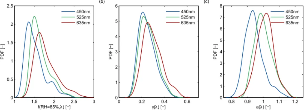
Figure 2.Probability density function (PDF) of(a)the measuredf(RH=85 %),(b)the fit-parameterγ (magnitude off(RH)) and(c)the fit-parametera(intercept). The different lines show the result for the three nephelometer wavelengths.
The surface residence time of an air parcel was then cal-culated by adding the travel time of each trajectory for the entire measurement period on a 1◦×1◦longitudinal and
lati-tudinal grid. Only periods when the air parcel was within the ML were considered.
To further differentiate between the continental and mar-itime influence the parameterψis introduced:
ψ=
tend
Z
tstart
(ρ(t )·ǫ(t ))dt, (4)
wheretstartdenotes the start andtend the arrival time of the trajectory. The factor ǫ(t )in Eq. (4) is+1 if the air parcel
traverses within the ML above land, while it is−1 when the
parcel traverses within the ML above oceans. The factorρ(t )
accounts for the removal of the particles with an estimated half-lifetime of one week (assuming a quadratic decrease with time). Other removal mechanisms (e.g. due to precipita-tion) are not taken into account. By this definition,ψhas as
outer boundaries−1 (air mass traversed only above oceans)
and+1 (air mass traversed only above land). We are aware
that this is a simplified way of classifying the air masses;
however, it will be shown thatψ sufficiently describes the
maritime and continental influence for our purposes.
5 Results
Section 5.1 describes the results of in situ measurements of
f(RH). Its correlation and the proposed parametrization to
the particle’s chemical composition are discussed in Sect. 5.2 and 5.3. The following Sect. 5.4 explains the extrapolation of the ground-based in situ measurements to the atmospheric column and compares the result to routinely performed SPM measurements. Different hypothesis are discussed in Sect. 6 that can impact the comparison.
5.1 Influence of water uptake on the aerosol light scattering coefficient at Hyytiälä
The time series off(RH) at RH=85 % was calculated by
av-eraging the humidograms every 3 h (one full RH cycle) and applying Eq. (2) to the measurements. The result is shown in Fig. 1 together with the corresponding dry scattering coefficient σsp, dry for λ=525 nm. f(RH=85 %, 525 nm)
Table 1.Mean, standard deviation (SD) and percentile values (prctl.) of the scattering enhancement factor f(RH), the magnitudeγ and interceptaof the fitted humidograms.
Mean SD 90th prctl. 75th prctl. Median 25th prctl. 10th prctl.
f(85 %, 450 nm) 1.53 0.24 1.90 1.64 1.47 1.35 1.26
f(85 %, 525 nm) 1.63 0.22 1.95 1.74 1.57 1.48 1.42
f(85 %, 635 nm) 1.79 0.27 2.17 1.94 1.71 1.59 1.51
γ(450 nm) 0.24 0.07 0.34 0.28 0.22 0.19 0.16
γ(525 nm) 0.25 0.07 0.35 0.29 0.24 0.20 0.17
γ(635 nm) 0.30 0.08 0.41 0.35 0.28 0.23 0.20
a(450 nm) 0.96 0.07 1.07 1.00 0.95 0.91 0.88
a(525 nm) 1.01 0.05 1.08 1.04 1.00 0.97 0.94
a(635 nm) 1.01 0.05 1.08 1.05 1.01 0.98 0.95
Table 2.Mean, standard deviation (SD) and percentile values (prctl.) of the particle light scattering coefficient (σsp,dry), the particle light
absorption coefficient (σap,dry), the single scattering albedo (ω0), the Ångström scattering exponent (αsp, determined by a fit) and the main
aerosol chemical components (ACSM and EC/OC analysis). All optical properties are given at dry conditions and were calculated to the
wavelength of the WetNeph nephelometer. The values are given for the time period when the WetNeph was in operation (see Fig. 1).
Mean SD 90th prctl. 75th prctl. Median 25th prctl. 10th prctl.
σsp,dry(450nm) [Mm−1] 42.03 25.42 79.57 52.91 34.07 22.84 18.35
σsp,dry(525nm) [Mm−1] 32.90 19.75 61.18 40.84 26.61 18.15 14.60
σsp,dry(635nm) [Mm−1] 27.19 17.65 51.01 34.34 21.27 14.62 11.00
σap,dry(450nm) [Mm−1] 2.11 1.19 3.45 2.54 1.90 1.32 0.92
σap,dry(525nm) [Mm−1] 1.82 1.00 3.05 2.22 1.62 1.14 0.82
σap,dry(635nm) [Mm−1] 1.51 0.82 2.63 1.89 1.35 0.94 0.66
ωsp,dry(450nm) [-] 0.95 0.02 0.97 0.96 0.95 0.93 0.91
ωsp,dry(525nm) [-] 0.94 0.03 0.97 0.96 0.94 0.93 0.91
ωsp,dry(635nm) [–] 0.94 0.03 0.97 0.96 0.94 0.93 0.91
αsp[-] 1.30 0.23 1.60 1.44 1.31 1.18 1.00
Organic mass conc. [µgm−3] 4.57 2.63 9.03 6.30 3.78 2.59 1.71
NH4mass conc. [µgm−3] 0.37 0.15 0.57 0.46 0.36 0.26 0.20
SO4mass conc. [µgm−3] 0.85 0.37 1.29 1.04 0.83 0.55 0.40
NO3mass conc. [µgm−3] 0.20 0.11 0.37 0.26 0.16 0.12 0.10
Cl mass conc. [µgm−3] 0.01 0.01 0.02 0.01 0.01 0.00 0.00
EC mass conc. [µgm−3] 0.13 0.07 0.20 0.14 0.11 0.09 0.07
a mean value of 1.63±0.22. f(RH=85 %, 525 nm)
de-creases with increasing dry scattering coefficientσsp, dry,
in-dicating an increased presence of less hygroscopic particles at highσsp, dry. The probability density function (PDF) of the measured f(RH=85 %) for all nephelometer wavelengths
and the entire campaign is shown in Fig. 2 together with the PDF of the fit parameters used in Eq. (2). A small increase of f(RH=85 %) with increasing wavelength is observed,
similar to observations made at Melpitz, Germany (Zieger et al., 2014). This effect can be reproduced by calculating the optical properties using Mie theory with the input of the measured size distribution and chemical composition of the particles. The fit-parametersγ andaconsequently show
a low variation with a mean and SD value of 0.25±0.07 and
1.01±0.05 respectively. The value ofa≈1 indicates the
ab-sence of hysteresis effects. The mean, SD and percentile val-ues off(RH=85 %) are given for all wavelengths in Table 1
together with the fit parameters (see Eq. 2). To bring our mea-surement results into a broader context, Table 2 shows the average values for the main aerosol optical parameters (all calculated to the nephelometer wavelengths) and the chemi-cal composition measurements.
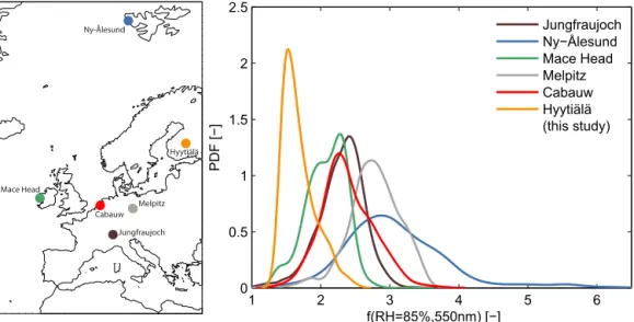
Thef(RH) observed at Hyytiälä is remarkably low
com-pared to other sites. Figure 3 shows the PDF at RH=85 %
and λ=550 nm (linearly interpolated) in comparison to
Ny-Ålesund
Mace Head
Jungfraujoch Melpitz Cabauw
Hyytiälä
1 2 3 4 5 6
0 0.5 1 1.5 2 2.5
f(RH=85%,550nm) [−]
PDF [−]
Jungfraujoch Ny−Ålesund Mace Head Melpitz Cabauw Hyytiälä (this study)
Figure 3.Probability density function (PDF) of the measuredf(RH=85 %, 550 nm) at Hyytiälä (orange line) in comparison to results obtained at other European sites where the same instrument had been deployed (see legend; data taken from Zieger et al., 2013). The result for Hyytiälä was linearly interpolated to 550 nm wavelength. The left panel shows the location of the different sites.
different nephelometer was used (Zieger et al., 2013). High values of f(RH) were measured for pristine maritime and
Arctic aerosol found at Ny-Ålesund, Spitsbergen (campaign mean and SD: f(85 %, 550 nm)=3.24±0.63), or aerosol
dominated by inorganic salts as recorded in winter 2009 at Melpitz, Germany (f(85 %, 550 nm)=2.77±0.37).
Inter-mediate values were usually measured for continental and anthropogenic influenced aerosol at Cabauw, the Nether-lands (f(85 %, 550 nm)=2.38±0.38), or free tropospheric
aerosol at Jungfraujoch, Switzerland (f(85 %, 550 nm)=
2.30±0.33). Thef(RH) values given above are campaign
av-erages; however, each site had its characteristics for specific air mass types like marine aerosol, anthropogenic-influenced aerosol or desert dust. For example, Mace Head in Ireland showed distinct differences inf(RH) depending on the wind
direction; if the air had a maritime origin generally higher values were observed (f(85 %, 550 nm)=2.28±0.19) in
contrast to wind coming from the island or continent with influence of anthropogenic emissions (f(85 %, 550 nm)=
1.80±0.26). A separation of different air mass types for the
other sites are given in Table 2 in Zieger et al. (2013). The trajectory analysis reveals further insights to the source of f(RH) as shown in Fig. 4. Only concurrent
times when all main in situ instruments (WetNeph, ACSM and aethalometer) were running in parallel were used. Fig-ure 4a reveals that the main catchment area of the air arriv-ing at Hyytiälä was southern Finland, Russia, the Baltic Sea, parts of Scandinavia and continental Europe as well as the Atlantic and Arctic oceans. Thef(RH=85 %, 525 nm), the
organic mass fraction and the EBC concentration were sepa-rately averaged on a 1◦×1◦grid when the air parcel of the
trajectory was within the ML for each grid point. It is hereby assumed that the property did not change along the
trajec-tory. It can be seen in Fig. 4b that air masses with eastern and continental origin had generally a lowerf(RH), while air
masses traversing over oceans or originating from the Arctic were characterized with elevated values off(RH), which can
be explained by the contribution of hygroscopic sea spray particles transported to Hyytiälä. However, no distinct del-iquescence was observed in contrast to other sites like Mel-pitz (Germany), Cabauw (The Netherlands) or Ny-AAlesund (Spitzbergen), which can be explained by the high contribu-tion of organic substances at Hyytiälä. Figure 4c shows the organic mass fraction is clearly elevated for continental air masses, while it decreased for air masses having a maritime origin. Figure 4d shows the spatial distribution of the EBC as measured by the aethalometer. A strong source of EBC around St. Petersburg in Russia and generally elevated con-centrations of air masses coming from the continent can be seen. No weighting or removal was considered for this analy-sis since mainly intensive parameters are shown. In addition, the analysis is also influenced by shadowing effects when air masses from different origin are averaged on the same grid point to one mean value. This can be avoided by using the factorψ introduced in Eq. (4), which reveals the potential
maritime and continental influence. Figure 5 shows the aver-age values off(RH=85 %, 525 nm), the EBC concentration
and the organic mass fraction vs.ψ. It can be seen that the
scattering enhancement is generally higher for maritime air masses, while it clearly decreases with increasing continen-tal influence. As an opposite trend, the organic mass fraction steadily increases with more continental influence. The EBC values show no significant trend compared tof(RH) or the
organic mass fraction.
Figure 4. Results of the trajectory analysis (10-day backward calculations of air masses arriving at Hyytiälä, black cross, averaged on a 1◦×1◦grid).(a)Total surface residence time,(b)scattering enhancement factor (at RH=85 % and 525 nm),(c)organic mass fraction,
(d)equivalent black carbon concentration. Only concurrent times are shown when all instruments were operated in parallel.
Maritime-continental influence Maritime-continental influence Maritime-continental influence
(a) (b) (c)
1 1.5 2 2.5
−0.75 to −0.5−0.5 to −0.25−0.25 to 00 to 0.250.25 to 0.50.5 to 0.750.75 to 1
f(RH=85%,525nm) [−]
0 100 200 300 400 500 600 700 800 900
−0.75 to −0.5−0.5 to −0.25−0.25 to 00 to 0.250.25 to 0.50.5 to 0.750.75 to 1
BC [ng/m
3]
0.1 0.2 0.3 0.4 0.5 0.6 0.7 0.8 0.9 1
−0.75 to −0.5−0.5 to −0.25−0.25 to 00 to 0.250.25 to 0.50.5 to 0.750.75 to 1
Organic mass fraction [−]
Maritime ContinentalMaritime ContinentalMaritime Continental
No. of points:
2 263 337 450 445 386 128
meteorological parameters. No clear and significant depen-dency was found when compared to the single scattering albedo, aerosol size distribution parameters (total number concentration and mean size), wind direction or wind speed. An exception was the small inverse correlation (R2= 0.45)
that was found for the scattering Ångström exponent (only when using the 450 and 525 nm scattering coefficients) and the total particle surface area. This can probably be ex-plained by the fact that an increased concentration of mainly smaller particles (increased Ångström exponent) were also composed of more organic components (lower hygroscop-icity), which overall caused a decreasedf(RH). This is also
seen in the trajectory analysis, which revealed that air masses from the east showed generally a higher Ångström exponent similar to the organic mass fractionForg(see Fig. 4c).
5.2 Comparison to the chemical composition measurements
The reason for the lowf(RH) at Hyytiälä can be explained
by the dominance of organic substances in the particle’s chemical composition, which leads to lower particle hygro-scopicity. As an example, the fit-parameter γ (Eq. 2) at λ=525 nm is plotted in Fig. 6 as a function of the
or-ganic mass fractionForg. The linear regression shows a clear anti-correlation (squared Pearson’s correlation coefficient:
R2=0.77) with a decrease in γ with increasing Forg (i.e.
γ (525nm)=(−0.71±0.15)·Forg+(0.76±0.11); retrieved
from a weighted bivariate fit according to York et al., 2004, taking the SD of the average values as an input for the un-certainty calculation). The dominance of the organic mass fraction (mean±SD: 0.7±0.11) clearly determines the low
values ofγ and thus the lowf(RH) observed at Hyytiälä.
For comparison, the values measured at Melpitz, Germany, are added to Fig. 6 (for more details see Zieger et al., 2014). The organic mass fraction at Melpitz of submicrometer par-ticles was substantially lower than at Hyytiälä (mean±SD:
0.23±0.10). Although theγ values for Melpitz were
mea-sured at a different time of year (winter) and showed a higher variability (R2=0.50), they almost line up linearly with
the observations made at Hyytiälä. Due to measurement re-strictions the total mass at Melpitz was only differentiated between black and organic carbon, while the total mass at Hyytiälä is determined from the elemental carbon of the EC/OC analysis (organic carbon is assumed to be included
in the ACSM organic mass fraction). The ammonia mass fractions at Hyytiälä and Melpitz are also linearly correlated, while the sulphate mass fraction did not show a joint lin-ear behaviour with the Melpitz data. The reason is that the aerosol found at Melpitz during the winter months also con-tained large amounts of nitrate which mainly formed am-monium nitrate (with a higher hygroscopicity than organic aerosol), while the nitrate contribution at Hyytiälä was very small and the sulphate mainly formed ammonium sulphate
0 0.2 0.4 0.6 0.8 1
0 0.2 0.4 0.6 0.8 1
Organic mass fraction Forg [−]
γ
(525nm) [−]
Melpitz (Zieger et al., 2014) Hyytiälä (this study)
Hyytiälä:γ=(−0.71±0.15) Forg + (0.76±0.11), R
2=0.77
Melpitz:γ=(−1±0.54) Forg + (0.79±0.14), R2 =0.5
Joint dataset: γ=(−0.67±0.066) Forg + (0.73±0.045), R2=0.9
Figure 6.The fit-parameterγ(forλ=525 nm) vs. the organic mass fractionForgmeasured at Hyytiälä (green bullets) and Melpitz,
Ger-many (grey squares). The solid and dashed lines represent the cor-responding bivariate weighted linear regressions.
or ammonium bisulphate, which together with the organic contribution lead to a generally lower hygroscopicity. 5.3 A simplified parametrization forf(RH)
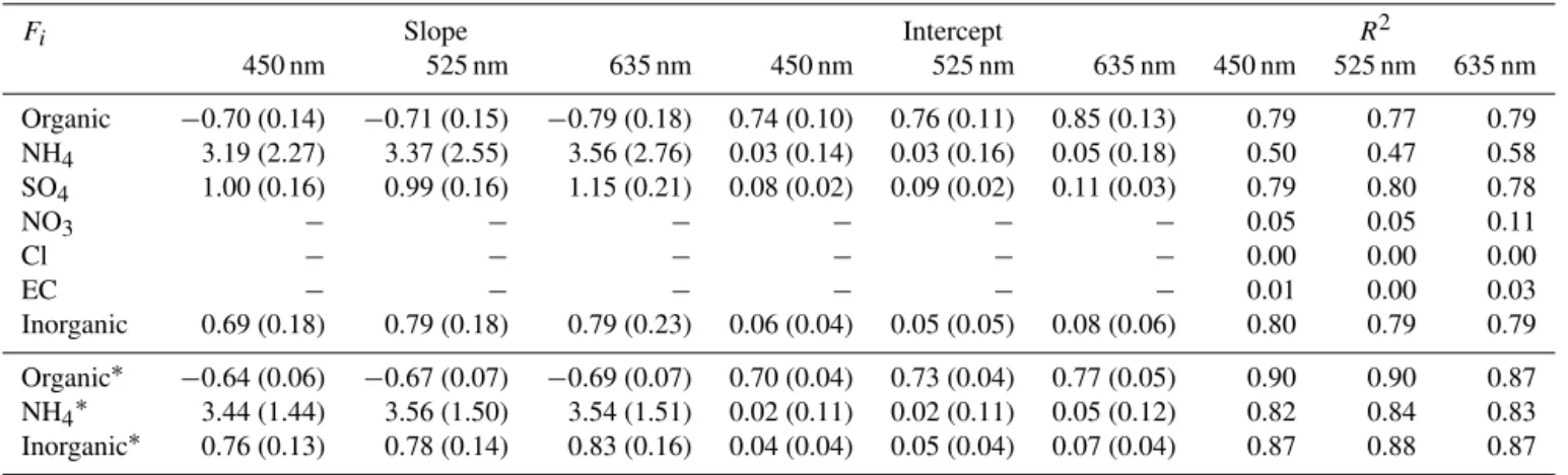
A summary of the linear fit parameters ofγ vs. the
chem-ical mass fractions is shown in Table 3 for the components which showed a clear linear behaviour. The inorganic mass fractions, mainly sulphate and ammonia, are clearly posi-tively correlated withγ andf(RH), in contrast to the
anti-correlated organic mass fraction. This allows the use of con-tinuously performed chemical composition measurements at Hyytiälä to predictf(RH) whether a humidified
nephelome-ter is operated. It can be done by taking the total organic or inorganic mass fraction as a proxy forf(RH) and using the
linear regression parameters given in Table 3 to calculateγ
for each wavelengths.f(RH) then follows by using Eq. (2),
assuming an intercept ofa=1. The variance of the intercept a can be used to estimate an uncertainty of thef(RH)
pre-diction (see Table 1).
Numerical parametrizations of f(RH) using chemical
mass fractions are only sparsely published. Quinn et al. (2005) proposed a similar parametrization of γ using
the mass fraction of organic matter and sulphate (γs= −0.6·Feorg+0.9 with Feorg=Corg/(Corg+CSO4)and γs=
ln(f (RH))/ln((1−RHref)/(1−RH)), which is similar to
Eq. (2) ifa=1; RHrefdenotes the dry reference RH). This
parametrization is limited to aerosol dominated by the accu-mulation mode and is only given forλ=550 nm (P. Quinn,
personal communication, May 2015). Our results (if cal-culated in the same manner as described in Quinn et al., 2005) show the same decreasing trend ofγs (for example for
Table 3.Parameters retrieved from a linear regression of the different chemical mass fractionsFi (ACSM and EC/OC) vs.γ(fit parameter forf(RH)) for the different nephelometer wavelengths. The calculated uncertainty of slope and intercept of the used bivariate weighted fit (York et al., 2004) are given in parenthesis. The parameters for NO3, Cl and EC are not given due to the low correlation. The lower part (marked by an asterisk) shows the linear regression parameters calculated in the same manner for the joint data set of Hyytiälä (this study) and Melpitz (Zieger et al., 2014) for the components which showed a joint linear behaviour. These values can be used to predictf(RH) by using Eq. (2) (assuming an intercept ofa=1).
Fi Slope Intercept R2
450 nm 525 nm 635 nm 450 nm 525 nm 635 nm 450 nm 525 nm 635 nm
Organic −0.70 (0.14) −0.71 (0.15) −0.79 (0.18) 0.74 (0.10) 0.76 (0.11) 0.85 (0.13) 0.79 0.77 0.79
NH4 3.19 (2.27) 3.37 (2.55) 3.56 (2.76) 0.03 (0.14) 0.03 (0.16) 0.05 (0.18) 0.50 0.47 0.58
SO4 1.00 (0.16) 0.99 (0.16) 1.15 (0.21) 0.08 (0.02) 0.09 (0.02) 0.11 (0.03) 0.79 0.80 0.78
NO3 − − − − − − 0.05 0.05 0.11
Cl − − − − − − 0.00 0.00 0.00
EC − − − − − − 0.01 0.00 0.03
Inorganic 0.69 (0.18) 0.79 (0.18) 0.79 (0.23) 0.06 (0.04) 0.05 (0.05) 0.08 (0.06) 0.80 0.79 0.79
Organic∗ −0.64 (0.06) −0.67 (0.07) −0.69 (0.07) 0.70 (0.04) 0.73 (0.04) 0.77 (0.05) 0.90 0.90 0.87
NH4∗ 3.44 (1.44) 3.56 (1.50) 3.54 (1.51) 0.02 (0.11) 0.02 (0.11) 0.05 (0.12) 0.82 0.84 0.83
Inorganic∗ 0.76 (0.13) 0.78 (0.14) 0.83 (0.16) 0.04 (0.04) 0.05 (0.04) 0.07 (0.04) 0.87 0.88 0.87
e
Forg+0.81 atλ=525 nm). However, both data sets do not
show the same joint linear trend anymore because the organic mass fraction of the parametrization by Quinn et al. (2005) is calculated using the organic and sulphate concentrations only. The aerosol at Melpitz, however, had a significant con-tribution of nitrate, ammonia and black carbon which needs to be included in the parametrization to retrieve a reliable estimate on f(RH). In a more recent study, Zhang et al.
(2015) parametrized their measurements off(RH) from the
Yangtze River Delta region in China in a similar way as Quinn et al. (2005) but adding also nitrate to the organic mass fraction. A linear relationship ofγs= −0.42·Feorg+0.54 with
e
Forg=Corg/(Corg+CSO4+CNO3)was found, which com-pares better to our results; however, the ammonia and black carbon components are still missing in the linear relationship presented by Zhang et al. (2015).
Table 3 also states the linear regression parameters for the joint Hyytiälä and Melpitz data sets. As mentioned above, the organic and the total inorganic mass fractions showed a common linear behaviour and thus a more general rule to predictf(RH) from aerosol chemical composition
measure-ments can be derived. Individual inorganic components like sulphate or nitrate may show different functional dependen-cies individually for each site; however, as the comparison to Quinn et al. (2005) and Zhang et al. (2015) showed, it is im-portant to include all major chemical constituents when de-riving a general parametrization ofγ orf(RH) as has been
done here. Our parametrization for Hyytiälä is strictly spo-ken only valid for the summer months when the fine mode is clearly dominated by less hygroscopic organic substances. Verification during other seasons and adding other sites is needed to allow a generalization of these findings. The addi-tion of the Melpitz findings from Zieger et al. (2014) should
only be seen as a first step. Additionally, the parametrization may not be valid during periods with substantially different coarse mode contribution which can have a potentially large impact on the totalf(RH) (Zieger et al., 2013).
5.4 Extrapolation to the atmospheric column using aircraft measurements
The in situ measurements were extrapolated to the atmo-spheric column using regular airborne profile measurements that were performed during the second half of May un-til mid of June 2013. In total 17 profiles with collocated cloud-free SPM measurements on the ground were avail-able. The measurements were binned in 200 m wide height levels (starting at 200 m a.s.l.). The profile flights time took on average 2.5 h and included up to three full ascends and descends. A comparison of the aircraft measurement at the lowest flight level (200–400 m a.s.l.) to the ground-based CPC shows a good agreement (R2=0.80, linear regression: NtotCessna=1.17Ntotground−142 cm−3) and slightly less
parti-cles by the ground CPC.
The AOD is defined as the vertical integral of the particle light extinction coefficientσep:
AOD(λ)= h1
Z
h0
σep(λ, h)dh, (5)
whereh0is the surface altitude,h1is usually the top of the atmosphere (e.g. when measured by a SPM) andλthe
wave-length. Here, h1 is the height of the highest profile point reached by the aircraft.
(aethalometer) were first transformed to the respective SPM wavelength using the Ångström law:
σsp(λ)=kλ−αsp, (6)
where k is the turbidity coefficient and αsp the scattering Ångström exponent. Equation (6) can be formulated for
σap,dry in an analogous way. The sum ofσsp,dry andσap,dry yields the particle light extinction coefficientσep,dry. We have limited the extrapolation to SPM wavelengths that are close to the nephelometer wavelengths to reduce the involved un-certainties. The in situ AODs are therefore only calculated between 440 and 870 nm. To calculateσep,dry(λ, h)at
differ-ent altitudes the total particle number concdiffer-entration Ntotas measured by the airborne CPC was used as a scaling factor
c (h). The in situ AOD for the dry case then calculates as
follows
AODin situdry (λ)= h1
Z
h0
c (h) σep, dryground(λ)dh,
with c (h)= Ntot(h)
Ntot(h0). (7)
For the ambient in situ AOD, the particle hygroscopic growth at RH of the different altitudes was now taken into account by using the ground-based measured f(RH) and
assuming that it does only depend on RH. This assump-tion means that the particle chemical composiassump-tion and inten-sive size distribution parameter do not change with altitude. Eq. (7) then changes to
AODin situamb. (λ)= h1
Z
h0
c (h)f (RH, λ)σsp, dryground(λ)
+σap, dryground(λ)dh. (8)
Note that the absorption coefficient is assumed not to change with RH. This is a reasonable assumption at Hyytiälä due to the fact that the scattering enhancement ex-ceeds the absorption enhancement (Nessler et al., 2005) and, even more importantly, due to the dominance of the light scattering (i.e. campaign average for the single scattering albedoω0=0.94±0.03 atλ=525 nm, see Table 2), which
in total will only induce a small error. Thef(RH) is linearly
inter- or extrapolated to the SPM wavelengths. To test the in-fluence of the layer above the maximum flight altitude an ex-ponential decrease of the total number concentration was as-sumed (withc(h)=c(hi)exp(−0.25h)above the maximum
flight altitude, where c(hi)is the scaling factor of the last
height bin and hthe altitude up to 7 km). This is a
reason-able assumption only for cases without clear elevated layers, which was most likely only given for the first half of the air-borne observation period (see Sect. 6.4). The in situ AOD with the exponential decreasing profile above the maximum
(b) (a)
0 20 40 60 80 100
0 500 1000 1500 2000 2500 3000 3500 4000 4500 RH [%]
0 2 4 6 8
x 10−5 0 500 1000 1500 2000 2500 3000 3500 4000 4500 σ
ep(λ=500nm) [m−1]
Altitude [m a.s.l.]
0 20 40 60 80 100
0 500 1000 1500 2000 2500 3000 3500 4000 4500 RH [%]
0 0.5 1 1.5 2
x 10−5 0 500 1000 1500 2000 2500 3000 3500 4000 4500 σ
ep(λ=500nm) [m −1]
Altitude [m a.s.l.]
RH Ground (amb.) c(h)*σ ep ground (dry) c(h)*σ ep ground (amb.) c(h)*σ ep ground (dry, extrp.)
Legend see (a)
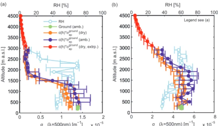
Figure 7.Example of the ground-based in situ measurements ex-trapolated to the atmospheric column. Particle light extinction coef-ficientσep(atλ=500 nm) measured at the surface at ambient RH (along the tower at 17, 67 and 124 m; green bullets), surface ex-tinction coefficient weighted with the relative changes in the total number concentration measured by the aircraft CPC (dry, orange points) and at ambient conditions (violet points) with the RH mea-sured on board the aircraft (blue points, upper axis). The red points are dry values ofσepabove the maximum flight altitude assuming
an exponential decreasing particle concentration. The error bars de-note the 25th and 75th percentile values.(a)Result for the 23 May 2013.(b)Result for the 02 June 2013.
flight level is only calculated for the dry case since no RH measurements are available above the maximum flight alti-tude.
To calculate the in situ AOD the atmosphere above was separated into 200 m wide levels in which the CPC measure-ments were averaged to determinec(h)for each layer starting
at 200 m a.s.l. (close to the top of the canopy and location of the SPM). Two example profiles showing the in situ derived profiles are presented in Fig. 7. For comparison, the ambi-ent extinction coefficiambi-ent measured at the ground is shown together with the RH profile. As a test for the variability, the calculations were repeated by using the 25th and 75th percentiles as lower and upper boundary respectively. In the first example, the top of the ML is clearly seen at around 1500 m. The particle light extinction coefficient sharply de-creases above the ML. The RH effect is significant but not very strong due to the low hygroscopicity of the organic-dominated aerosol at Hyytiälä and the low RH profile during that time of day (RH varied within the ML between 50 and 70 % while it decreased to 20 % above 2000 m). Integrating the ambient extinction coefficient profile yields an AODin situ amb. of 0.018 atλ=500 nm, while the SPM measured a value of
0.055. The second profile example (Fig. 7b) shows the re-sult for the 02 June, where no clear ML transition can be observed. The extinction coefficient still is elevated even at the maximum flight level of 2700 m. An integration of the ambient extinction coefficient profile gives an AODin situamb. of 0.1 atλ=500 nm, while the SPM measured a value of 0.37.
1000 2000 3000 4000
Max. flight alt. [m]
(a)
0 0.05 0.1 0.15 0.2 0.25 0.3 0.35 0.4
AOD(
λ
=500nm) [−]
(b)
Sun photometer (SPM) In−situ (dry) In−situ (amb.) In−situ (dry, extrp.)
−100 −50
0
Relative diff. to SPM AOD(
λ
=500nm) [%]
(c)
In−situ (dry) In−situ (amb.) In−situ (dry, extrp.)
05/19 05/26 06/02 06/09 06/16
−100 −50
0
Relative diff. to SPM
AOD(
λ
) [%]
(d)
λ=870 nm
λ=675 nm
λ=500 nm
λ=440 nm
Figure 8. (a)Time series of the maximum altitude during the aircraft profiling.(b)Time series of the AOD atλ=500 nm measured by the sun photometer (SPM, grey curve), determined from the ground-based dry extinction coefficient and the airborne CPC as scaling factor (orange curve) and determined from the ground-based extinction coefficient at ambient conditions (violet curve). The red dashed curve represents the in situ derived AOD when an exponential decreasing profile is assumed above the maximum flight altitude (at dry conditions). The error bars denote the distance to the 25th and 75th percentile values, while the centre point gives the median value for each profile.(c)
Relative difference of in situ derived AOD compared to the SPM measurement ((AODin-situ−AODSPM)/AODSPM·100% atλ=500 nm).
(d)Relative difference of dry in situ derived AOD compared to the SPM measurement for different SPM wavelengths.
SPM measured ones are depicted in Fig. 8 forλ=500 nm
to-gether with the maximum flight altitude. The in situ derived values follow the course in time of the direct AOD values of the SPM. However, they are 2–3 times smaller than the di-rectly obtained ones (Fig. 8c). Figure 8b and c also reveals that the addition of an assumed exponential decreasing pro-file above approx. 3 km only marginally leads to an increase of the in situ derived dry AOD. This points towards the fact that most of the particles were captured by the aircraft profil-ing, if the assumption of an exponential decrease in particle number concentration is valid. However, this assumption is most likely not valid for the second half of the aircraft profil-ing period. As can be seen in Fig. 8b, the AOD increases in the beginning of June due to long-range transport of mineral dust in elevated layers (see Sect. 6.4). The WetNeph was not in continuous operation between 08 and 15 June 2013 due to computer failures and thus the ambient AODin situamb. was not retrieved for this period.
The calculations were done for all SPM wavelengths be-tween 440 and 870 nm which are close to the spectral region of the nephelometer. Figure 8d shows that the relative
differ-ence of the dry in situ derived AOD to the SPM measured values increases for larger wavelengths. These differences are more pronounced for the period of potential long-range transported mineral dust.
The following hypotheses are brought forward to explain the clear disagreement between in situ derived and directly measured AOD:
1. assumptions made to calculate AODin-situ; 2. inconsistencies within the in situ measurements; 3. missing coarse mode particles (Dp>1 µm) and general
sampling losses within the ground-based in situ mea-surements;
4. removal by dry deposition within the canopy; 5. aerosol layers above the maximum flight altitude.
6 Discussion
6.1 Influence of general assumptions being made The main assumptions that were made in Sect. 5.4 can all have a potential influence on the disagreement between in situ derived and measured AOD values. The first main as-sumption is to use the total particle number concentration as scaling factorc(h)in Eqs. (7) and (8). It should be noted here
that the results are in a similar range if the particle surface is being used to calculatec(h); however, that factor would omit
optically active particles above the upper size limit of the air-borne SMPS (see Fig. 11b) and therefore we prefer to take the total concentration to determinec(h).
To calculate the ambient extinction, it was assumed in Eq. (8) that the particle light absorption enhancement is neg-ligible. As mentioned above, this is justified for this site due to the low absorption enhancement effect compared to the scattering effect and the overall dominance of particle light scattering when determining the particle light extinction co-efficient (Nessler et al., 2005).
For the ambient case, it was additionally assumed that the
f(RH) is the same within the column as measured at ground
and therefore only depends on the RH at different altitudes. This assumption implies that the chemical composition (hy-groscopicity) and mean size is constant throughout the at-mospheric column. This assumption is most likely fulfilled for a well-mixed boundary layer; however, it will not be valid for lofted or separate layers during episodes with long-range transported air masses. During the summer months at Hyytiälä, however, the columnar RH was always moderate and low in addition to the fact that particles are generally less hygroscopic at this boreal site and, therefore, the overall effect of the constantf(RH) assumption was probably small
compared to the hypotheses discussed below. 6.2 Consistency of in situ measurements: optical
closure study
To prove the consistency of the optical and microphysical aerosol in situ measurements, a closure study based on Mie theory (Bohren and Huffman, 2004) was performed. The particles were assumed to be spherical, homogeneous and internally mixed. As input, the particle number size dis-tribution measured by the DMPS and APS was used (the APS and DMPS size distributions were merged at the last DMPS size bin). The complex refractive index was inverted from the dry scattering (nephelometer) and absorption coef-ficient (aethalometer) measurements and the measured parti-cle number size distribution using Mie theory (Zieger et al., 2010). Only the measurements from the continuous aerosol monitoring program were used for the retrieval since they were also located inside the aerosol cottage. The calculation was done incorporating the TSI nephelometer illumination sensitivity and the specific scattering angles to avoid the
trun-cation error (Anderson et al., 1996). Forλ=450 nm a mean
value for the RI of(1.56±0.07)+(0.008±0.005)iwas
cal-culated, while(1.53±0.06)+(0.008±0.005)iand(1.50±
0.07)+(0.008±0.005)iwere calculated forλ=550 nm and λ=700 nm respectively. These retrieved real parts of the RI
for Hyytiälä are close to the values of ammonium sulphate (e.g. 1.536+10−7iatλ=450 nm; Toon et al., 1976). The
re-sult of the Mie calculations is shown in Fig. 9a, in which the relative differences between prediction (Mie calculation) and measurement are shown for all nephelometer wavelengths. The monitoring nephelometer (located in the cottage) is in almost perfect agreement to the calculation which is reason-able since the same measurement was used to retrieve the RI. However, the little variation proves that it is justified to use an average and fixed RI for each wavelength for the entire period. The calculatedσsp,dryfor the dry nephelometer used
within the WetNeph system (located in the campaign con-tainers) are clearly underestimated by the model calculations (on average 8–30 %, see Fig. 9a). This corresponds to gen-eral differences between the dry monitoring nephelometer in the cottage measuring less particle light scattering than the reference nephelometer of the WetNeph located inside the container (see Fig. 9b). The lower measured scattering coef-ficients of the cottage nephelometer are in correspondence to the underestimation of the measured particle number size dis-tribution, which is an input to the Mie calculation. Therefore, particle number concentration and light scattering measure-ments of the monitoring measurement inside the cottage were affected by the same loss effect. Almost the same result is obtained when the RI of ammonium sulphate is taken. Small parts of the disagreement could come from general calibra-tion issues of the nephelometers used in the WetNeph set-up. The larger variation of the WetNeph reference nephelometer (the error bars denote the 25th and 75th percentile values) suggests that the container site experienced more variation in aerosol concentration compared to the cottage site inside the forest.
The differences in the scattering coefficients cancel out when the scattering enhancement is calculated. In a first test, the hygroscopic growths factors g(RH) (Eq. 3) of the
HT-DMA were taken (details on thef(RH) calculation can be
found in Zieger et al., 2013). The g(RH) values were
in-terpolated between the measured dry diameters ofDp=30
and 145 nm. Above 145 nm, the values ofg(RH) were
as-sumed to be the same as the one measured atDp=145 nm
(similar forDp=30 nm). The calculated values of f(RH)
using the HTDMA measurements lie on average within the range of the measured values (Fig. 9a). A slight disagree-ment for the larger wavelengths (on average 12 % at 635 nm) is found. As second test, the values ofg(RH) were calculated
using the ACSM and EC/OC measurements. The value for
pure organics was first assumed to begorg(RH=90 %)=1.2
(Fierz-Schmidhauser et al., 2010b; Zieger et al., 2014) and secondly assumed to begorg(RH=90 %)=1.05, a value
(a) (b)
−80 −60 −40 −20 0 20 40 60 80
Difference (Neph1 − Neph2)/ Neph2 x 100 [%]
Nephelometer comparison (dry)
σ
sp,dry(λ) measured
Neph1: cottage Neph2: container −80
−60 −40 −20 0 20 40 60 80
Difference (predicted−measured)/measured x 100 [%] σsp(λ) dry
Neph cottage with RI of Mie inversion
σ sp(λ) dry
Neph container with RI of Mie inversion
f(RH=85%,λ)
with g(RH) of HTDMA
f(RH=85%,λ)
with g(RH) of ACSM+EC/OC g
org(90%)=1.2
f(RH=85%,λ)
with g(RH) of ACSM+EC/OC g
org(90%)=1.05
Optical closure (Mie calculation)
450nm 525nm 635nm 450nm (cottage) 550nm (cottage) 700nm (cottage)
Figure 9. (a)Result of the optical closure study. Relative differences of the predicted to measured scattering coefficient (dry) and scattering enhancement factor (at RH=85 %) for the different nephelometer wavelengths. The circle denotes the median value and the error bars the 25th and 75th percentile values.(b)Comparison of the dry nephelometer measurements (σsp,dry) between cottage (monitoring) and container
(WetNeph). The values of the cottage nephelometer were interpolated using Eq. (6).
(Riipinen et al., 2015). The calculated values using the origi-nal value ofgorg(RH=90 %)=1.2 are systematically higher
than the direct measurements (≈30 %), while the lower
value ofgorg(RH=90 %)=1.05 delivers an improved
agree-ment. This points towards the importance of the hygroscopic growth factor, which is especially for low hygroscopic sub-stances important when calculating f(RH) (see Fig. A1 in
Zieger et al., 2013).
Summarizing the optical closure study, one can conclude that the different in situ measurements provide consistent re-sults. However, the differences found in the scattering coeffi-cients measured by the monitoring and reference nephelome-ters point towards losses. Partitioning effects of semi-volatile organics (Donahue et al., 2006) or nitrate components (due to the low concentration to a lesser extent, see Table 2) that could have caused a potential decrease in the overall particle properties cannot be ruled out completely. Although it is be-lieved to have a minor effect during the summer months and daytime in situ measurements at this site. Smaller differences can additionally be explained by the simplified assumptions taken for the Mie calculations (e.g. internal mixture, homo-geneous and spherical particles, no size dependence of the refractive index, specific values forg(RH)).
6.3 Particle losses
The SPM was placed on a tower above the forest canopy (∼198 m a.s.l.), while the in situ measurements were
per-formed on ground below the canopy (∼180 m a.s.l.).
Parti-cles may have been lost within the canopy by dry deposi-tion before reaching the inlet (Grönholm et al., 2007; Bu-zorius et al., 2003; Petroff et al., 2008), which includes re-moval through Brownian diffusion (mainly for fine mode par-ticles belowDp<100 nm) or through impaction or
intercep-tion (mainly for coarse mode particles aboveDp>1000 nm).
Grönholm et al. (2009) performed aerosol flux measurements using the eddy covariance technique at Hyytiälä and found that only 35 % of the particles penetrated through the canopy at low wind speeds. At higher wind speeds and correspond-ingly stronger turbulent conditions only 10 % of all particles reached the ground. The study by Grönholm et al. (2009) was performed in spring, while our measurements were done in summer months with probably more turbulence and thus higher deposition losses. In addition, particle losses could have also occurred within the inlet and tubing itself. How-ever, this is rather unlikely since the optical closure study has shown the consistency of the optical and microphysical aerosol measurements.
Figure 10a shows the average particle number size distri-bution measured at the ground and by the aircraft within the lowest layer. For small particles below 100 nm, the aircraft measured on average higher concentrations (up to 40 %) than the ground-based instrument. However, for the optically im-portant size range above 100 nm, both size distributions agree surprisingly well. Figure 10b depicts the scattering size dis-tribution calculated using the measured size disdis-tributions and Mie theory. Here, both size distribution measurements agree until the maximum diameter of the aircraft SMPS is reached. Unfortunately, aboveDp>270 nm the aircraft did not record
the size distribution and thus missed information on the opti-cally important part of the aerosol size spectrum.
The relative disagreement between in situ derived and measured AOD values increased for larger wavelengths (see Fig. 8d), which points towards an influence of large parti-cles which are not sufficiently sampled by the in situ instru-ments. Figure 11 shows the calculated scattering coarse mode fraction (defined as the scattering coefficient for particles aboveDp>1 µm divided by the total scattering coefficient
101 102 103 0
500 1000 1500 2000 2500 3000 3500 4000
Particle diameter [nm]
dN/dlogD [cm
−3] (a)
Ground Airborne
101 102 103
0 1 2 3 4 5 6 7 8x 10
−5
λ=500nm
Particle diameter [nm]
d
σ
/dlogD [m
−1] (b)
Ground Airborne
Figure 10. (a) Average particle number size distribution measured at ground and within the lowest flight level by the aircraft (200– 400 m a.s.l.).(b) Aerosol scattering size distribution calculated using Mie theory for the wavelengths of 500 nm (RI=1.51). The centre lines show the median, while the corresponding shaded areas denote the 25th and 75th percentile values.
400 600 800 1000 1200 1400 1600
0 0.2 0.4 0.6 0.8 1
Wavelength [nm]
σsp
(D
p
>1
µ
m)/
σsp
(tot) [−]
Figure 11.Coarse mode fraction of the particle light scattering co-efficient vs. the sun photometer wavelengths. The black centre line shows the median value, while the shaded area denote the 25th and 75th percentile value range for the period with airborne measure-ments.
in the SPM measurements. The calculation was done for all time periods with corresponding profiles using the particle number size distribution measurement on the ground. With increasing wavelength more light scattering will be due to coarse mode particles. Atλ=1020 nm, for example, it is
al-ready 50 % for the here measured aerosol. A few losses of supermicron particles can therefore explain the observed dif-ferences.
The AOD for the fine mode fraction (Dp<1 µm) was
esti-mated by taking the measured particle number size distribu-tion at ground and applying Mie theory (taking the RI from the Mie inversion, see Sect. 6.2) which results in the extinc-tion coefficient for submicrometer particles only. The calcu-lation of in situ AOD for the fine mode fraction followed in the same manner as described above (using Eq. 8). The comparison of the derived values to the AERONET inverted fine mode AOD is shown in Fig. 12. A high correlation was
0 0.05 0.1 0.15 0.2
0 0.05 0.1 0.15 0.2 0.25
y=1.53x+0.0239
R2= 0.84
Fine mode AOD(500nm) in−situ (ambient) [−]
Fine mode AOD(500nm) AERONET [−]
Figure 12.Aerosol optical depth (AOD) of fine mode particles de-rived from AERONET vs. the in situ dede-rived value using Mie the-ory and the measured size distribution (at 550 nm). The error bars denote the range of the 25th and 75th percentile values, while the centre points mark the median value.
found (R2=0.84) and a linear least-squares regression
re-vealed that the AERONET values were significantly higher (slope of 1.53) compared to the in situ derived values. Again, this indicates that besides the missing coarse mode also the loss of fine mode particles contributed to the found disagree-ment. These particles could have been fine mode particles above the maximum flight altitude (see Sect. 6.4) or particles possibly lost through dry deposition within the canopy. 6.4 Elevated layers