NPGD
1, 543–582, 2014Improving ETKF using the second-order
information
G. Wu et al.
Title Page
Abstract Introduction
Conclusions References
Tables Figures
◭ ◮
◭ ◮
Back Close
Full Screen / Esc
Printer-friendly Version Interactive Discussion
Discussion
P
a
per
|
D
iscussion
P
a
per
|
Discussion
P
a
per
|
Discuss
ion
P
a
per
|
Nonlin. Processes Geophys. Discuss., 1, 543–582, 2014 www.nonlin-processes-geophys-discuss.net/1/543/2014/ doi:10.5194/npgd-1-543-2014
© Author(s) 2014. CC Attribution 3.0 License.
Open Access
Nonlinear Processes in Geophysics
Discussions
This discussion paper is/has been under review for the journal Nonlinear Processes in Geophysics (NPG). Please refer to the corresponding final paper in NPG if available.
Improving the ensemble transform
Kalman filter using a second-order Taylor
approximation of the nonlinear
observation operator
G. Wu1, X. Zheng1, L. Wang2, X. Liang3, S. Zhang1, and X. Zhang1
1
State Key Laboratory of Remote Sensing Science, College of Global Change and Earth System Science, Beijing Normal University, Beijing, China
2
Department of Statistics, University of Manitoba, Winnipeg, Canada
3
National Meteorological Information Center, China Meteorological Administration, Beijing, China
Received: 28 January 2014 – Accepted: 12 March 2014 – Published: 11 April 2014
Correspondence to: X. Zheng ([email protected])
NPGD
1, 543–582, 2014Improving ETKF using the second-order
information
G. Wu et al.
Title Page
Abstract Introduction
Conclusions References
Tables Figures
◭ ◮
◭ ◮
Back Close
Full Screen / Esc
Printer-friendly Version Interactive Discussion
Discussion
P
a
per
|
D
iscussion
P
a
per
|
Discussion
P
a
per
|
Discuss
ion
P
a
per
|
Abstract
The Ensemble Transform Kalman Filter (ETKF) assimilation scheme has recently seen rapid development and wide application. As a specific implementation of the Ensemble Kalman Filter (EnKF), the ETKF is computationally more efficient than the conventional EnKF. However, the current implementation of the ETKF still has some limitations when 5
the observation operator is strongly nonlinear. One problem is that the nonlinear op-erator and its tangent-linear opop-erator are iteratively calculated in the minimization of a nonlinear objective function similar to 4DVAR, which may be computationally expen-sive. Another problem is that it uses the tangent-linear approximation of the observation operator to estimate the multiplicative inflation factor of the forecast errors, which may 10
not be sufficiently accurate.
This study seeks a way to avoid these problems. First, we apply the second-order Taylor approximation of the nonlinear observation operator to avoid iteratively calculat-ing the operator and its tangent-linear operator. The related computational cost is also discussed. Second, we propose a scheme to estimate the inflation factor when the 15
observation operator is strongly nonlinear. Experimentation with the Lorenz-96 model shows that using the second-order Taylor approximation of the nonlinear observation operator leads to a reduction of the analysis error compared with the traditional lin-ear approximation. Similarly, the proposed inflation scheme leads to a reduction of the analysis error compared with the procedure using the traditional inflation scheme. 20
1 Introduction
The spatial and temporal distribution of observations is continuously changing with the improvement of numerical models and observation techniques. Sounding data, remote sensing observations, radiance data and other indirect information bring both opportu-nities and challenges in data assimilation. How to assimilate these indirect observations 25
NPGD
1, 543–582, 2014Improving ETKF using the second-order
information
G. Wu et al.
Title Page
Abstract Introduction
Conclusions References
Tables Figures
◭ ◮
◭ ◮
Back Close
Full Screen / Esc
Printer-friendly Version Interactive Discussion
Discussion
P
a
per
|
D
iscussion
P
a
per
|
Discussion
P
a
per
|
Discuss
ion
P
a
per
|
The observation operators for indirect observations are often nonlinear. For example, radiative transfer codes (e.g., RTTOV, CRTM, Saunders et al., 1999; Han et al., 2006) can be treated as observation operators by mapping air temperature and moisture to the microwave radio brightness temperature (McNally, 2009). Because the relationship of these observations with modelled variables may be strongly nonlinear (Liou, 2002), 5
and because the observation errors may be spatially correlated (Miyoshi et al., 2013), data assimilation schemes have to be appropriately designed to address such indirect observations.
Most data assimilation methods are fundamentally based on linear theory but have different responses to departures from linearity (Lawson and Hansen, 2004). Con-10
ceptually, variational data assimilation schemes (VAR, e.g., Parrish and Derber, 1992; Courtier et al., 1994; Lorenc, 2003) can assimilate data with nonlinear observation op-erators and spatially correlated observation errors. However, a drawback of VAR is that it has to calculate the adjoint of a dynamical model, which is not an easy task in prac-tice. Moreover, VAR does not give a direct estimate of the background error covariance 15
matrix, which is crucial for the performance of any data assimilation scheme.
The Ensemble Kalman Filter (EnKF) scheme has a strategy to optimize forecast er-ror statistics without using the adjoint of the dynamical model (e.g., Evensen, 1994a, 1994b; Burgess et al., 1998; Anderson and Anderson, 1999; Wang and Bishop, 2003; Wu et al., 2013). It is also conceptually applicable to data assimilation with nonlinear 20
observation operators. However, it has been demonstrated that when the observation operator is strongly nonlinear, using the linear approximation of the observation oper-ator to derive the error covariance evolution equation can result in an oversimplified closure and dubious performance of the EnKF (e.g., Miller et al., 1994; Evensen, 1997; Yang et al., 2012).
25
NPGD
1, 543–582, 2014Improving ETKF using the second-order
information
G. Wu et al.
Title Page
Abstract Introduction
Conclusions References
Tables Figures
◭ ◮
◭ ◮
Back Close
Full Screen / Esc
Printer-friendly Version Interactive Discussion
Discussion
P
a
per
|
D
iscussion
P
a
per
|
Discussion
P
a
per
|
Discuss
ion
P
a
per
|
matrix through eigenvector decomposition of a matrix with the ensemble size. Hunt et al. (2007) extended the ETKF method to address a general nonlinear observation operator using the cost function, similar to Lorenc (2003). However, Hunt et al. (2007) minimized the weight vector of the ensemble analysis state instead of the analysis state, as in Lorenc (2003). In addition to the reduction of the computational cost com-5
pared with EnKF, another advantage of the ETKF proposed by Hunt et al. (2007) is that it can assimilate observations with strongly nonlinear observation operators (Chen et al., 2009) and with spatially correlated observation errors (Stewart et al., 2013), sim-ilar to VAR.
However, there are still problems associated with the ETKF when the observation 10
operator is strongly nonlinear. First, the current ETKF is based on the minimization of a cost function similar to that in VAR for nonlinear observation operators (Hunt et al., 2007). The direct calculation for the minima may be computationally expensive because the nonlinear operators and their tangent-linear operators have to be itera-tively calculated. Using the linear approximation of the nonlinear observation operators 15
(e.g. Hunt et al., 2007) can effectively reduce the computational burden, but at the cost of increasing analysis error. Second, tangent-linear approximation of the observation operator is used for the forecast error inflation in the ETKF (e.g., Li et al., 2009). If the observation operators are strongly nonlinear, the inflation factors and hence the fore-cast error covariance matrices may be estimated erroneously in this way, leading to an 20
eventual increase in the analysis error.
In this study, we propose two alternative approaches to improving assimilation quality when the observation operator is strongly nonlinear. First, in an effort to reduce compu-tational cost without significantly reducing estimation quality, we use the second-order Taylor expansion of the observation operator to estimate both the inflation factors and 25
NPGD
1, 543–582, 2014Improving ETKF using the second-order
information
G. Wu et al.
Title Page
Abstract Introduction
Conclusions References
Tables Figures
◭ ◮
◭ ◮
Back Close
Full Screen / Esc
Printer-friendly Version Interactive Discussion
Discussion
P
a
per
|
D
iscussion
P
a
per
|
Discussion
P
a
per
|
Discuss
ion
P
a
per
|
The potential use of the second-order information has been noted by some authors. For example, Hunt et al. (2007) noted that the second-order derivatives of the objec-tive function might be used to estimate the covariance of analysis weight, which is an important step in ETKF with a nonlinear observation operator. Moreover, Le Dimet et al. (2002) and Daescu and Navon (2007) noted that the second-order information in 5
nonlinear variational data assimilation is important to the issue of solution uniqueness. In the conventional ETKF scheme, the linear approximation of nonlinear observa-tion operators is used for the purpose of reducing the computaobserva-tional cost compared with conventional methods of searching the minima of nonlinear cost functions (Hunt et al., 2007). This study also aims to investigate the changes of analysis errors when 10
a nonlinear observation operator is substituted by its first-order and second-order Tay-lor approximations. We focus on the formulation of the forecast error inflation method in the case of a nonlinear observation operator and on improved accuracy with the second-order vs. the first-order approximation and the linear approximation. Further studies on the performance of the proposed schemes in practical data assimilations 15
are needed and should be performed in the future.
The remainder of the paper is organized as follows. Our modified ETKF schemes are described in Sect. 2. The assimilation results on a Lorenz-96 model with a nonlinear observation system are presented in Sect. 3. The discussions are given in Sect. 4, and conclusions are presented in Sect. 5.
20
2 Methodology
2.1 ETKF with forecast error inflation
NPGD
1, 543–582, 2014Improving ETKF using the second-order
information
G. Wu et al.
Title Page
Abstract Introduction
Conclusions References
Tables Figures
◭ ◮
◭ ◮
Back Close
Full Screen / Esc
Printer-friendly Version Interactive Discussion
Discussion
P
a
per
|
D
iscussion
P
a
per
|
Discussion
P
a
per
|
Discuss
ion
P
a
per
|
Using the notations of Ide et al. (1997), a nonlinear discrete-time forecast and obser-vation system can be written as
xti =Mi−1(xai−1)+ηi, (1)
yoi =Hi(xti)+εi, (2)
5
where i is the time step index; xti ={xit(1),xit(2),. . .,xti(n)}T is the n-dimensional true state vector; xai−1={xia−1(1),xia−1(2),. . .,xia−1(n)}T is the n-dimensional analy-sis state vector, which is an estimate of xti−1; Mi is the nonlinear forecast
oper-ator; yoi ={yio(1),yio(2),. . .,yio(pi)}T is the pi-dimensional observation vector; Hi =
{hi(1),hi(2)···,hi(pi)}Tis the nonlinear observation operator, where hi(k) is a n
-10
dimensional multivariate function; and ηi and εi are the forecast and observation
er-ror vectors, which are assumed to be statistically independent of each other, time-uncorrelated, and to have mean zero and covariance matrices Pi and Ri, respec-tively. The detailed procedure of the ETKF with a nonlinear observation operator (Hunt et al., 2007) with the proposed inflation scheme is as follows.
15
Step 1. Calculate thejth perturbed forecast state at timei as
xfi,j=Mi−1 xai−1,j
, (3)
wherexai−1,j is thejth perturbed analysis state at timei−1. Then, the mean forecast state is defined as
20
xfi = 1
m m X
j=1
xfi,j, (4)
wheremis the total number of ensemble members.
Step 2. Assume the forecast errors to be in the formpλi(xfi,j−xfi), (j=1, 2,. . .,m), where the inflation factorλi can be estimated by minimizing the objective function
25
Li(λ)=Tr
didTi −Ci(λ)−I didTi −Ci(λ)−I T
NPGD
1, 543–582, 2014Improving ETKF using the second-order
information
G. Wu et al.
Title Page
Abstract Introduction
Conclusions References
Tables Figures
◭ ◮
◭ ◮
Back Close
Full Screen / Esc
Printer-friendly Version Interactive Discussion
Discussion
P
a
per
|
D
iscussion
P
a
per
|
Discussion
P
a
per
|
Discuss
ion
P
a
per
|
Here,Iis them×midentity matrix,
di =R−i 1/2yoi −Hi xfi
. (6)
is the innovation vector normalized by the square root of the observation error covari-ance matrix (Wang and Bishop, 2003), and
5
Ci(λ)≡ 1
m−1
m X
j=1 h
R−i 1/2 Hi xfi +pλ xfi,j−xfi
−Hi xfi
Hi xfi + p
λ xfi,j−xfi
−Hi xfi T
R−i1/2i. (7)
(See Appendix A for details).
Step 3. Calculate the analysis state as 10
xai =xfi + q
ˆ
λiXfiwai (8)
where
Xfi = xfi,1−xfi,xfi,2−xfi,. . .,xfi,m−xfi (9) 15
andwai is estimated by minimizing the objective function
Ji(w)=1
2(m−1)w
Tw +1
2
yoi −Hi
xfi + q
ˆ
λiXfiw
T
R−i 1
yoi −Hi
xfi + q
ˆ
λiXfiw
. (10)
Step 4. Calculate a perturbed analysis state as 20
xai,j=xai + q
ˆ
NPGD
1, 543–582, 2014Improving ETKF using the second-order
information
G. Wu et al.
Title Page
Abstract Introduction
Conclusions References
Tables Figures
◭ ◮
◭ ◮
Back Close
Full Screen / Esc
Printer-friendly Version Interactive Discussion
Discussion
P
a
per
|
D
iscussion
P
a
per
|
Discussion
P
a
per
|
Discuss
ion
P
a
per
|
where Wai,j is the jth column of the matrix Wai =√m−1( ¨Ji|wai)−
1/2
and ¨Ji|wai is the second-order derivative ofJi(w) atwai (see Appendix B for details). Lastly, seti =i+1 and return to Step 1 for the next iteration.
For estimating the inflation factor, Li et al. (2009) proposed a scheme, for which the tangent-linear operator of the observation operator (see Sect. 2.2.1 for the definition) 5
is required. In the effort to reduce computational cost of searching the minima of the objective function (Eq. 10), Hunt et al. (2007) suggested the following linear approxi-mation,
Hi
xfi + q
ˆ
λiXfiw
≈Hi xfi
+Yfiw (12)
10
where
Yfi =
Hi q
ˆ
λi xfi,1−xfi
+xfi
−Hi xfi
,Hi q
ˆ
λi xfi,2−x f i
+xfi
−Hi xfi
,
. . .,Hi q
ˆ
λi xfi,m−xfi +xfi
−Hi xfi
. (13)
In this study, this traditional ETKF approach is validated against the other approaches. 15
2.2 Simplified estimation methods in special cases
To compute the variational minimization in Eq. (10) operationally, one can directly com-pute the explicit solution of the minima and iterate the process as in the 4D-Var outer loop (Lorenc, 2003; Liu et al., 2008). However, doing so still requires repeatedly cal-culating the nonlinear function Hi(xfi +
q
ˆ
λiXfiw) and its tangent-linear operator (see
20
NPGD
1, 543–582, 2014Improving ETKF using the second-order
information
G. Wu et al.
Title Page
Abstract Introduction
Conclusions References
Tables Figures
◭ ◮
◭ ◮
Back Close
Full Screen / Esc
Printer-friendly Version Interactive Discussion
Discussion
P
a
per
|
D
iscussion
P
a
per
|
Discussion
P
a
per
|
Discuss
ion
P
a
per
|
2.2.1 First-order Taylor approximation forHi
The first-order Taylor approximation forHi at the forecast state vectorxfi is defined as
Hi xti
≈Hi xfi +H˙i|xf
i x
t i−x
f i
, (14)
where 5
˙ Hi|xf
i =
∂hi(1)
∂xi(1) ···
∂hi(1)
∂xi(n) ..
. . .. ...
∂hi(pi)
∂xi(1) ···
∂hi(pi)
∂xi(n)
xi=xfi
(15)
is the first-order derivative ofHi evaluated at the forecast statexfi (tangent-linear
oper-ator). Then,λi can be estimated by minimizing the quadratic function
L1,i(λ)=Trh didiT−λR−i1/2H˙i|xf i
ˆ PiH˙Ti|xf
iR
−1/2 i −I
10
didTi −λRi−1/2H˙i|xf i
ˆ PiH˙Ti|xf
iR
−1/2 i −I
Ti
. (16)
The analytic solution is
ˆ
λi =
TrhR−i 1/2H˙i|xf i
ˆ PiH˙Ti|xf
iR
−1/2 i did
T i −I
Ti
TrhR−i1/2H˙i|xf i
ˆ PiH˙Ti|xf
iR
−1
i H˙i|xfiPˆiH˙ T i|xfiR
−1/2 i
i, (17)
15
where
ˆ
NPGD
1, 543–582, 2014Improving ETKF using the second-order
information
G. Wu et al.
Title Page Abstract Introduction Conclusions References Tables Figures ◭ ◮ ◭ ◮ Back Close
Full Screen / Esc
Printer-friendly Version Interactive Discussion Discussion P a per | D iscussion P a per | Discussion P a per | Discuss ion P a per |
Similarly,wai can be estimated by minimizing the multivariate quadratic function
J1,i(w)=
1
2(m−1)w
T
w
+1
2
yoi −Hi xfi
−
q
ˆ
λiH˙i|xfiXfiw
T
R−i1
yoi −Hi xfi
−
q
ˆ
λiH˙i|xfiXfiw
(19)
and the analytic solution is 5
wai = (m−1)I+λˆ XfiTH˙Ti|xf iR
−1 i H˙i|xfiXfi
−1 q
ˆ
λi Xfi T˙
HTi|xf iR
−1 i y
o
i −Hi x f i
. (20)
(see Appendix C for details).
2.2.2 Second-order Taylor approximation forHi
The second-order Taylor approximation forHi atxfi is defined as
10
Hi xti
≈Hi xfi +H˙i|xf
i x
t i−x
f i +1 2 x t i −x
f i
T
⊗H¨i|xf i ⊗ x
t i−x
f i
, (21)
whereH¨i|xf i ≡ {
¨ Hi|xf
i(1),. . .,
¨ Hi|xf
i(pi)}
T
is the second-order derivative ofHi atxfi,
¨ Hi|xf
i(k)≡
∂2hi(k)
∂xi(1)∂xi(1) ···
∂2hi(k)
∂xi(1)∂xi(n)
..
. . .. ...
∂2hi(k)
∂xi(n)∂xi(1) ···
∂2hi(k)
∂xi(n)∂xi(n)
xi=xfi
k=1,. . .,pi, (22)
15
and⊗is the outer product operator, i.e., for two arbitraryn-dimensional vectorsxand
y,
xT⊗H¨i|xf
i ⊗y={x
TH¨
i|xfi(1)y,. . .,xTH¨i|xfi(pi)y} T
NPGD
1, 543–582, 2014Improving ETKF using the second-order
information
G. Wu et al.
Title Page Abstract Introduction Conclusions References Tables Figures ◭ ◮ ◭ ◮ Back Close
Full Screen / Esc
Printer-friendly Version Interactive Discussion Discussion P a per | D iscussion P a per | Discussion P a per | Discuss ion P a per |
is a pi-dimensional vector. Then, λi can be estimated by minimizing the polynomial objective function ofλ1/2
L2,i(λ)=Trh didiT−λR−i1/2H˙i|xf i
ˆ PiH˙Ti|xf
iR
−1/2 i −λ
3/2C
1,i−λ3/2CT1,i−λ 2C
2,i−I
didTi −λRi−1/2H˙i|xf i
ˆ PiH˙Ti|xf
iR
−1/2 i −λ
3/2C
1,i−λ3/2CT1,i−λ 2C
2,i−I Ti
, (24) 5
where
C1,i = 1
2(m−1)
m X
j=1
R−i 1/2H˙i|xf i
q
λi xfi,j−xfi
xfi,j−xfiT⊗H¨i|xf i ⊗ x
f i,j−x
f i
T
R−i 1/2
, (25)
and 10
C2,i = 1
4(m−1)
m X
j=1 h
R−i1/2 xfi,j−xfiT⊗H¨i|xf
i ⊗ x
f i,j−x
f i
xfi,j−xfiT⊗H¨i|xf i ⊗ x
f i,j−x
f i
T
R−i 1/2
. (26)
Moreover, wai can be estimated by minimizing the multivariate polynomial objective function
15
J2,i(w)≈
1
2(m−1)w
Tw
+1
2
"
yoi −Hi xfi
−
q
ˆ
λiH˙i|xfiXfiw− ˆ
λi
2
XfiwT⊗H¨i|xf
i ⊗ X
f iw
#T
R−i1
"
yoi −Hi xfi
−
q
ˆ
λiH˙i|xfiXfiw− ˆ
λi
2
XfiwT⊗H¨i|xf
i ⊗ X
f iw
#
NPGD
1, 543–582, 2014Improving ETKF using the second-order
information
G. Wu et al.
Title Page
Abstract Introduction
Conclusions References
Tables Figures
◭ ◮
◭ ◮
Back Close
Full Screen / Esc
Printer-friendly Version Interactive Discussion
Discussion
P
a
per
|
D
iscussion
P
a
per
|
Discussion
P
a
per
|
Discuss
ion
P
a
per
|
(see Appendix D for details).
2.3 Validation statistics
In the following experiments, the “true” statexti is known by experimental design and is non-dimensional. In this case, we can use the Root Mean Square Error of the Analysis state (A-RMSE) to evaluate the accuracy of the assimilation results. The A-RMSE at 5
theith step is defined as
A-RMSE= r
1
nkx a i −x
t
ik2, (28)
where k · k denotes the Euclidean norm and n is the dimension of the state vector. A smaller A-RMSE indicates a better performance of the assimilation scheme.
10
Following Anderson (2007) and Liang et al. (2012), the Root Mean Square Error of the Forecast state (F-RMSE) and the Spread of the Forecast state (F-Spread) at the
ith step are defined as
F-RMSE= r
1
nkx f i −x
t
ik2. (29)
15
and
F-Spread= v u u t
1
n(m−1)
m X
j=1
kxfi,j−xfik2. (30)
Roughly speaking, if xfi,j and xti are identically distributed with a mean value of xfi, then F-RMSE and F-Spread should be consistent with each other. This is more likely 20
NPGD
1, 543–582, 2014Improving ETKF using the second-order
information
G. Wu et al.
Title Page
Abstract Introduction
Conclusions References
Tables Figures
◭ ◮
◭ ◮
Back Close
Full Screen / Esc
Printer-friendly Version Interactive Discussion
Discussion
P
a
per
|
D
iscussion
P
a
per
|
Discussion
P
a
per
|
Discuss
ion
P
a
per
|
3 Experiments with the Lorenz-96 model
In Sect. 2.1, we outlined the general ETKF assimilation scheme with Second-order Least Squares (SLS) error covariance matrix inflation. In Sect. 2.2, we proposed sim-plified estimation methods for two special cases: whenHi is tangent-linear (Sect. 2.2.1)
and whenHi can be approximated by the second-order Taylor expansion (Sect. 2.2.2). 5
In this section, we apply these assimilation schemes to the Lorenz-96 model (Lorenz, 1996) with model errors and a nonlinear observation system because it is a nonlinear dynamical system with properties relevant to realistic forecast problems.
3.1 Description of the dynamic and observation system
The Lorenz-96 model (Lorenz, 1996) is a strongly nonlinear dynamical system with 10
quadratic nonlinearity governed by the equation
dXk
dt =(Xk+1−Xk−2)Xk−1−Xk+F, (31)
wherek=1, 2,. . .,K (K =40, so there are 40 variables). We apply the cyclic boundary conditionsX−1=XK−1,X0=XK,XK+1=X1. The dynamics of Eq. (31) are
“atmosphere-15
like” in that the three terms on the right-hand side consist of a nonlinear advection-like term, a damping term and an external forcing term, respectively. These terms can be thought of as a given atmospheric quantity (e.g., zonal wind speed) distributed on a latitude circle.
We solve Eq. (31) using the fourth-order Runge–Kutta time integration scheme 20
NPGD
1, 543–582, 2014Improving ETKF using the second-order
information
G. Wu et al.
Title Page
Abstract Introduction
Conclusions References
Tables Figures
◭ ◮
◭ ◮
Back Close
Full Screen / Esc
Printer-friendly Version Interactive Discussion
Discussion
P
a
per
|
D
iscussion
P
a
per
|
Discussion
P
a
per
|
Discuss
ion
P
a
per
|
the fractal dimension of the attractor is 27.1 (Lorenz and Emanuel, 1998). The initial condition is chosen to beXk=F whenk6=20 andX20=1.001F.
Because the microwave brightness temperature is an exponential function of soil temperature, we use the exponential observation function to mimic the radiative transfer model in this study. Suppose the synthetic observation generated at thekth model grid 5
point is
yio(k)=xit(k) exp{αxti(k)}+εi(k), (32)
where k=1,. . .,pi, and εi ={εi(1),εi(2),. . .,εi(pi)}T is the observation error vector with a mean of zero and covariance matrixRi. Here,α is a parameter controlling the 10
nonlinearity of the observation operator, andα=0 corresponds to the linear case. All the 40 model variables are observed in our experiments. Suppose the observation errors are spatially correlated. The leading-diagonal elements ofRi areσo2=1, and the off-diagonal elements at site pair (j,k) are
Ri(j,k)=σo2×0.5min(|j−k|,40−|j−k|), (33)
15
With the exponential observation function and spatially correlated observation errors, the proposed scheme may potentially be applied to assimilate remote sensing obser-vations and radiance data.
We added model errors in the Lorenz-96 model because they are inevitable in real 20
dynamic systems. The model is a forced dissipative model with a parameterF that con-trols the strength of the forcing (Eq. 31). It behaves quite differently, with different values ofF, and it produces chaotic systems with integer values ofF larger than 3. Thus, we used various values ofF to simulate a wide range of model errors while retainingF =8 when generating the “true” state. These observations were then assimilated withF =4, 25
NPGD
1, 543–582, 2014Improving ETKF using the second-order
information
G. Wu et al.
Title Page
Abstract Introduction
Conclusions References
Tables Figures
◭ ◮
◭ ◮
Back Close
Full Screen / Esc
Printer-friendly Version Interactive Discussion
Discussion
P
a
per
|
D
iscussion
P
a
per
|
Discussion
P
a
per
|
Discuss
ion
P
a
per
|
3.2 Assimilation results
In this section, we examine the following five data assimilation methods corresponding to five different treatments of nonlinearity in inflation factor estimation and optimization:
ETKF: Traditional ETKF described in the last paragraph of Sect. 2.1.
TT: Tangent-linear approximation in both inflation (Eq. 17) and optimization (Eq. 20) 5
TN: Tangent-linear approximation in inflation (Eq. 17) and nonlinearity in optimization (Eq. 10)
SS: Second-order approximation in both inflation (Eq. 24) and optimization (Eq. 27) NN: Nonlinearity in both inflation (Eq. 5) and optimization (Eq. 10).
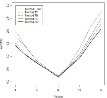
The corresponding time-mean A-RMSEs of these assimilation schemes withα=0.1 10
and F =4, 5, . . . , 12, over 100 000 time steps are plotted in Fig. 1. First, the figure clearly shows that for each estimation method, the A-RMSE increases asF becomes increasingly distant from the true value of 8.
Moreover, method NN has a smaller A-RMSE uniformly over all values of F than method TN, indicating that the proposed nonlinear inflation estimation (Eq. 5) per-15
forms better than the tangent-linear inflation scheme (Eq. 17). On the other hand, the A-RMSEs of methods SS and TN are close and smaller than that of method TT, sug-gesting that the second-order Taylor approximation method is comparable to the partial nonlinear method and is better than the first-order Taylor approximation method. Lastly, the traditional ETKF method has the largest A-RMSE, which implies that although the 20
linear approximation is computationally more efficient, it may introduce larger analysis error.
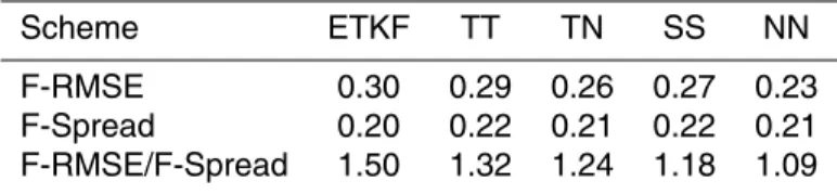
For the Lorenz-96 model with large error (F =12), the time-mean A-RMSEs and F-RMSEs of the five methods are given in Table 1 as well as the time-mean values of the objective functions. It can be seen that the full nonlinear method (NN) has both 25
NPGD
1, 543–582, 2014Improving ETKF using the second-order
information
G. Wu et al.
Title Page
Abstract Introduction
Conclusions References
Tables Figures
◭ ◮
◭ ◮
Back Close
Full Screen / Esc
Printer-friendly Version Interactive Discussion
Discussion
P
a
per
|
D
iscussion
P
a
per
|
Discussion
P
a
per
|
Discuss
ion
P
a
per
|
Taylor approximation method (TT). In all cases, a smaller error corresponds to a smaller value of the objective functionL.
To investigate the consistency between F-RMSE and F-Spread, we present the time-mean values of the five methods for casesF =12 andF =8 in Tables 2 and 3, respec-tively, as well as the ratios of F-RMSE over F-Spread. It is easy to see that in all cases, 5
the F-RMSEs are larger than F-Spreads, and therefore, all ratios are greater than 1. However, the ratio of the full nonlinear method (NN) is the smallest, while the ratio of the linear approximation method is the largest. The ratio of the second-order approx-imation method (SS) is comparable to that of the partial nonlinear method (TN), but smaller than that of the first-order approximation method (TT). This suggests that the 10
ensemble perturbed predictions are the most (least) reasonable for method NN (ETKF). Moreover, the ratios withF =8 are much closer to 1 than those withF =12 because the model error withF =12 is much larger than that withF =8 (see Sect. 2.3).
3.3 Impacts of Taylor approximations
In Sect. 3.2, we see that the A-RMSEs derived from the five ETKF assimilation 15
schemes are close when F is close to the true value of 8 but are different when F
departs from 8. This effect may depend on how well the Taylor expansions approxi-mate the nonlinear observation operatorHi.
For example, the Taylor expansion of the kth component of observation operator
Hi(x)=xexp{αx}(Eq. 32) withα=0.1 around the forecast statexif(k) is 20
xit(k) exp{0.1xti(k)}=xif(k) exp{0.1xfi(k)}
+ 1+0.1xif(k)exp{0.1xfi(k)} xti(k)−xfi(k)
+ 0.2+0.01xfi(k)
exp{0.1xif(k)} xti(k)−xif(k)2+···. (34)
To verify how well the Taylor expansions approximate the nonlinear observa-25
NPGD
1, 543–582, 2014Improving ETKF using the second-order
information
G. Wu et al.
Title Page
Abstract Introduction
Conclusions References
Tables Figures
◭ ◮
◭ ◮
Back Close
Full Screen / Esc
Printer-friendly Version Interactive Discussion
Discussion
P
a
per
|
D
iscussion
P
a
per
|
Discussion
P
a
per
|
Discuss
ion
P
a
per
|
xit(k) exp{0.1xti(k)}. If a ratio falls outside the interval [−0.1, 0.1], then the correspond-ing residual cannot be regarded as becorrespond-ing of a higher order infinitesimal and, therefore, cannot be ignored. Therefore, a larger proportion of the ratios falling outside the interval [−0.1, 0.1] indicates a worse Taylor expansion and vice versa.
The proportions of the ratios that fall outside the interval [−0.1, 0.1] are plotted 5
in Fig. 2, which shows that when F =8, the proportions are 0.0169 and 0.0006 for the first-order and second-order Taylor expansions, respectively. This result indicates that at almost all times and locations, both the first-order and second-order Taylor ex-pansions are good approximations of xti(k) exp{0.1xti(k)}. However, when F =12, at approximately 47 % (19 %) of the times and locations,xti(k) exp{0.1xti(k)} cannot be 10
adequately approximated by its first (second) order Taylor expansion. Therefore, the A-RMSEs derived by the five ETKF schemes are quite different. This example also indicates that the success of the Taylor approximation method depends on both the smoothness ofHi and the range of forecast states. It seems that for the same strongly
nonlinear observation operator, the larger the model error, the less success of the Tay-15
lor approximation.
4 Discussions
4.1 Inflation
It is widely recognized that the initial estimates of ensemble forecast errors should be inflated to improve assimilated results. To date, however, all of the existing adaptive 20
inflation schemes in ETKF are based on the assumption that the observation operator is linear or tangent-linear (e.g., Li et al., 2009; Miyoshi, 2011). In this study, a method to estimate the multiplicative inflation factors is proposed for general nonlinear obser-vation operators.
Historically, in systems such as the Met Office ETKF (Flowerdew and Bowler, 2011), 25
NPGD
1, 543–582, 2014Improving ETKF using the second-order
information
G. Wu et al.
Title Page
Abstract Introduction
Conclusions References
Tables Figures
◭ ◮
◭ ◮
Back Close
Full Screen / Esc
Printer-friendly Version Interactive Discussion
Discussion
P
a
per
|
D
iscussion
P
a
per
|
Discussion
P
a
per
|
Discuss
ion
P
a
per
|
analysis ensemble to be severely under-spread even when the background ensemble is well-spread. In this case, therefore, inflation must be applied to the analysis ensem-ble to correctly respond to the actual analysis uncertainty in the nonlinear forecast step. Inflation of the background ensemble may be more appropriate when the inflation pri-marily represents forecast model error, although stochastic physics or additive inflation 5
may be more appropriate in this case (Hamill and Whitaker, 2005; Wu et al., 2013). Our choice to inflate the background ensemble is crucial to the ability of finding a di-rect nonlinear solution for Eqs. (5)–(7) because of the way the inflation factor appears in these equations. Our objective function for estimating the multiplicative inflation factors is the second-order distance between the expectations of the squared innovation and 10
its realization, which also makes the rms spread equal to the rms error (e.g., Palmer et al., 2006; Wang and Bishop, 2003; Flowerdew and Bowler, 2011).
The proposed nonlinear method is tested using the Lorenz-96 model with nonlinear observation systems (Sect. 3.2). The resulting A-RMSEs are clearly smaller than those of the first-order Taylor approximation in the estimation of the inflation factor. This in-15
dicates that the proposed full nonlinear inflation method is better than the first-order Taylor approximation inflation method in the case of nonlinear observation operators (i.e., method NN is better than method TN). In addition, the F-RMSE and the F-Spread of the proposed nonlinear method are more consistent than those of the first-order Taylor approximation method.
20
The proposed inflation method works well in the case where observation errors are spatially correlated. Some data assimilation schemes assume the observation error covariance matrix to be diagonal for simplicity and ease of computation (e.g., Ander-son, 2007, 2009). However, because satellite observations often contain significantly correlated errors, the observation error covariance matrix has nonzero off-diagonal en-25
tries (Miyoshi et al., 2013). The inflation method proposed in this study can be applied to assimilate such observations.
NPGD
1, 543–582, 2014Improving ETKF using the second-order
information
G. Wu et al.
Title Page
Abstract Introduction
Conclusions References
Tables Figures
◭ ◮
◭ ◮
Back Close
Full Screen / Esc
Printer-friendly Version Interactive Discussion
Discussion
P
a
per
|
D
iscussion
P
a
per
|
Discussion
P
a
per
|
Discuss
ion
P
a
per
|
and Anderson, 1999). For testing the empirical tuning method, the most accurate ap-proach (i.e. estimate the minima of the objective function, Eq. 10), and the statistics root mean square errors of analysis-minus-observation and forecast minus-observation are used to tune the inflation factor. The A-RMSEs are estimated as 2.97 and 2.85 re-spectively which are larger than that of method SS (2.29). The ratios of F-RMSE to 5
F-Spread are estimated as 3.14 and 3.45 respectively, which are also larger than that of method SS (1.80). All these facts indicate than the empirical estimation method for the inflation factor is not as good as our proposed method in this experimentation.
4.2 Second-order Taylor approximation
In Sect. 3.2, we showed that the ETKF scheme equipped with our proposed nonlin-10
ear inflation method leads to the smallest A-RMSE in all ETKF schemes analysed in this study. However, this ETKF scheme requires repeated calculation of the nonlinear observation functionsHi(xfi +√λ(xi,jf −xfi)) andHi(xfi +
q
ˆ
λiXfiw) when minimizing the objective functionsLi(λ) andJi(w), which can be computationally expensive. To reduce
the computational cost, a commonly used approach is to substituteHi by its
tangent-15
linear operator (i.e., first-order Taylor expansion). However, this approach comes at the cost of losing estimation quality, as we have shown in this study.
As an effort to strike a balance between the estimation quality and computational cost, the nonlinear observation operatorHi in the objective functionsLi(λ) and Ji(w) is substituted by its order Taylor expansion. This is because (1) the second-20
order Taylor expansion is a better approximation ofHi than its tangent-linear operator;
(2) with second-order Taylor expansion, the inflation factor λ and the weight vector
w are concentrated out of Hi, so the objective functions (Eqs. 24 and 27) become polynomials, for which a minima is easier to derive; and (3) the second-order derivative ofHi is required for estimating ensemble analysis states (Eq. 11) in the ETKF scheme, 25
NPGD
1, 543–582, 2014Improving ETKF using the second-order
information
G. Wu et al.
Title Page
Abstract Introduction
Conclusions References
Tables Figures
◭ ◮
◭ ◮
Back Close
Full Screen / Esc
Printer-friendly Version Interactive Discussion
Discussion
P
a
per
|
D
iscussion
P
a
per
|
Discussion
P
a
per
|
Discuss
ion
P
a
per
|
The accuracy of the ETKF scheme with the second-order Taylor approximation is examined in Sect. 3.2. The results suggest that the scheme is more accurate than the ETKF scheme based on the first-order Taylor approximation and is comparable with the scheme based on nonlinear optimization and tangent-linear multiplicative inflation. However, it is less accurate than the nonlinear optimization and nonlinear inflation es-5
timation ETKF scheme proposed in this study. On the other hand, both schemes have similar F-RMSE over F-Spread ratios.
Despite the advantage that the objective functions (Eqs. 24 and 27) are easier to min-imize, the computational cost of the ETKF with the second-order Taylor approximation may increase from computing (Xfiw)TH¨i|xf
i,kX
f
iw. Because the most typical nonlinear
10
observation operator in numerical weather prediction is the radiative transfer model RT-TOV, the related computational issue is discussed and is documented in Appendix E. In fact, unlike forecast operators, the observation operators are usually localized, and therefore, the computation of (Xfiw)TH¨i|xf
i,kX
f
iw is still feasible.
In additional, there are other ways to address this problem. For example, in the deter-15
ministic variational framework, Met Office re-linearizes the observation operator every 10 iterations (Rawlins et al., 2007), and ECMWF uses a nonlinear outer loop. Both ap-proaches retain the efficiency of a tangent-linear approximation in the inner loop, while allowing for nonlinearity at a higher level. To better understand the efficacy of the ETKF scheme with second-order Taylor approximation, a more careful comparison with alter-20
native assimilation schemes is necessary. We plan to face this challenge in the near future.
4.3 Caveats
This study assumes the inflation factor to be constant in space, but this is apparently not the case in many practical applications, specifically when observations are sparse. 25
NPGD
1, 543–582, 2014Improving ETKF using the second-order
information
G. Wu et al.
Title Page
Abstract Introduction
Conclusions References
Tables Figures
◭ ◮
◭ ◮
Back Close
Full Screen / Esc
Printer-friendly Version Interactive Discussion
Discussion
P
a
per
|
D
iscussion
P
a
per
|
Discussion
P
a
per
|
Discuss
ion
P
a
per
|
2009; Miyoshi et al., 2010; Miyoshi and Kunii, 2012). If the forecast model has a large error, a multiplicative inflation may not be effective enough to improve the assimilation results. In this case, the additive inflation and localization technique may be applied to further improve the assimilation quality (Wu et al., 2013).
This study also assumes that the analysis increment can be expressed as a linear 5
combination of ensemble forecast errors (Eq. 8). This assumption is true if the ob-servation operator is tangent-linear, but the nonlinear obob-servation operator can affect the combination of possible increments that produce the optimal analysis (Yang et al., 2012). However, our examples demonstrate that the proposed ETKF methods can still work well when the observation operators are not tangent-linear.
10
At the last, but not the least, the results concluded in this study are related to the Lorenz-96 experiment. It may not be regarded as general rules. However, they can serve as counter examples to validate some ideas.
5 Conclusions
In this study, a new approach to inflating the ensemble forecast errors is proposed for 15
the ETKF with a nonlinear observation operator. For an idealized model, it is shown that the proposed inflation approach can reduce analysis error compared with the tangent-linear multiplicative inflation, despite it being computationally more expensive. An ETKF scheme with the second-order Taylor approximation is also proposed. In terms of anal-ysis error, the scheme is better than the first-order Taylor approximation ETKF scheme 20
and traditional ETKF scheme, specifically when the model error is larger. However, it is comparable to the scheme based on nonlinear optimization and tangent-linear multi-plicative inflation. Finally, the proposed ETKF scheme with nonlinear optimization and nonlinear inflation was found to be the best among all of the schemes presented in this study.
NPGD
1, 543–582, 2014Improving ETKF using the second-order
information
G. Wu et al.
Title Page
Abstract Introduction
Conclusions References
Tables Figures
◭ ◮
◭ ◮
Back Close
Full Screen / Esc
Printer-friendly Version Interactive Discussion
Discussion
P
a
per
|
D
iscussion
P
a
per
|
Discussion
P
a
per
|
Discuss
ion
P
a
per
|
In the future studies, we plan to further investigate the computational efficiency of the proposed ETKF schemes and to validate them using more sophisticated dynamic models and observation systems.
Appendix A
Derivation of Eq. (6)
5
The estimation of the inflation factorsλis based on the innovation statistic normalized by the square root of the observation error covariance matrix
di =R−i 1/2 yoi −Hi xfi =R−i 1/2 yoi −Hi xti
+R−i 1/2 Hi xti
−Hi xfi
, (A1) 10
whereyoi,xfi andxti are the observation, forecast and true state vector at theith time step, respectively, and Hi is the observation operator. The covariance matrix of the random vector di can be expressed as a second-order regression equation (Wang and Leblanc, 2008):
didTi =Eh Ri−1/2 yoi −Hi xti
+R−i1/2 Hi xti
−Hi xfi
15
R−i 1/2 yoi −Hi xti
+R−i1/2 Hi xti
−Hi xfiTi+Ξ, (A2)
whereEis the expectation operator andΞis a zero-mean error matrix. The expectation in Eq. (A2) has the decomposition
Eh R−i1/2 yoi −Hi xti
+R−i 1/2 Hi xti
−Hi xfi
20
R−i 1/2 yoi −Hi xti
+R−i1/2 Hi xti
NPGD
1, 543–582, 2014Improving ETKF using the second-order
information
G. Wu et al.
Title Page
Abstract Introduction
Conclusions References
Tables Figures
◭ ◮
◭ ◮
Back Close
Full Screen / Esc
Printer-friendly Version Interactive Discussion
Discussion
P
a
per
|
D
iscussion
P
a
per
|
Discussion
P
a
per
|
Discuss
ion
P
a
per
|
=EhR−i 1/2 yoi −Hi xti
yoi −Hi xti T
R−i1/2i
+EhR−i 1/2 Hi xti
−Hi xfi
Hi xti
−Hi xfi T
R−i 1/2i
+EhR−i 1/2 yoi −Hi xti
Hi xti
−Hi xfiTR−i1/2i
+EhR−i 1/2 Hi xti
−Hi xfi
yoi −Hi xitTR−i1/2i. (A3) 5
Assuming the forecast and observation errors are statistically independent, we have
EhR−i1/2 yoi −Hi xti
Hi xti
−Hi xfiTR−i1/2i
=R−i1/2Eh yoi −Hi xti
Hi xti
−Hi xfiTiR−i1/2=0, (A4)
EhR−i1/2 Hi xti
−Hi xfi
yoi −Hi xtiTR−i1/2i
=R−i1/2Eh Hi xti
−Hi xfi
yoi −Hi xtiTiR−i1/2=0. (A5) 10
From Eq. (2),yoi −Hi(xti) is the observation error at theith time step, and hence,
EhR−i1/2 yoi −Hi xti
yoi −Hi xtiTR−i1/2i
=R−i 1/2Eh yoi −Hi xti
yoi −Hi xtiTiR−i 1/2
=R−i 1/2RiR−i1/2
15
=I. (A6)
NPGD
1, 543–582, 2014Improving ETKF using the second-order
information
G. Wu et al.
Title Page
Abstract Introduction
Conclusions References
Tables Figures
◭ ◮
◭ ◮
Back Close
Full Screen / Esc
Printer-friendly Version Interactive Discussion
Discussion
P
a
per
|
D
iscussion
P
a
per
|
Discussion
P
a
per
|
Discuss
ion
P
a
per
|
Because the ensemble forecast states may be regarded as sample points ofxti (An-derson, 2007), we have
EhR−i1/2 Hi xti
−Hi xfi
Hi xti
−Hi xfiTR−i1/2i
= 1
m−1
m X
j=1 h
R−i1/2 Hi xfi +
p
λ xfi,j−xfi−Hi xfi
Hi xfi +pλ xfi,j−xfi
−Hi xfiTR−i1/2i
5
≡Ci(λ). (A7)
Substituting Eqs. (A3)–(A7) into Eq. (A2), we have
didTi =Ci(λ)+I+Ξ. (A8)
10
It follows that the second-order moment statistic of errorΞcan be expressed as
TrhΞΞTi=Trh didTi −Ci(λ)−I
didTi −Ci(λ)−ITi
≡Li(λ). (A9)
Appendix B
15
Derivation of ˙Ji|w and ¨Ji|w
The first-order derivative of the objective functionJi(w) (Eq. 10) is
˙
Ji(w)=(m−1)w−
q
ˆ
λi XfiTH˙T
i|xfi+ q
ˆ λiXfiw
R−i1
yoi −Hi
xfi + q
ˆ
λiXfiw
![Fig. 2. The proportions of residual ratios of the first-order and second-order Taylor expansions over the nonlinear observation operator x t i ,k exp {0.1x t i,k } that fall outside the interval [−0.1, 0.1], as a function of forcing F .](https://thumb-eu.123doks.com/thumbv2/123dok_br/16361219.190262/40.918.185.526.134.446/proportions-residual-expansions-nonlinear-observation-operator-interval-function.webp)
