On the Nonlinear Estimation of GARCH Models Using an Extended Kalman Filter

(1)

On the Nonlinear Estimation of GARCH Models

Using an Extended Kalman Filter

Sebasti´an Ossand´on and Natalia Bahamonde

Abstract—A new mathematical representation, based on a discrete-time nonlinear state space formulation, is presented to characterize a Generalized Auto Regresive Conditional Het-eroskedasticity (GARCH) model. Nonlinear parameter estima-tion and nonlinear state estimaestima-tion, for this state space model, using an Extended Kalman Filter (EKF) are described. Finally some numerical results, which make evident the effectiveness and relevance of the proposed nonlinear estimation are given.

Index Terms—GARCH models; Discrete-time nonlinear state space model; Nonlinear parameter estimation; Nonlinear state estimation; Extended Kalman Filter.

I. INTRODUCTION

During the last to decades GARCH type modeling, En-gle [5] and Bollerslev [2], has been an extremely active area of research. These models are often used in financial econometrics literature because their properties are close to the observed properties of empirical financial data. Also these propeties can capture various stylized facts. These models have gained popularity, specially due to their easy applicability and flexibility, allowing simple extensions that better fit the empirical financial data.

For the class of GARCH models, the most commonly used estimation procedure has been the Quasi Maximum Like-lihood (QMLE) aproach. Weiss [14] was the first to study the asymptotic properties of QMLE in GARCH models. The asymptotic properties of the QMLE for classical GARCH models have been extensively studied; see, for recent refer-ences, Berkes et al [1], Francq and Zakoian [6], Hall and Yao [8].

Alternatively, other estimation procedures are available based on the Autoregressive Moving Average Model (ARMA) representation of the squared GARCH process. This idea was taken by Giraitis and Robinson [7] who studied the Whittle estimator of parametric Auto Regresive Conditional Heteroskedasticity(∞)(ARCH(∞)) models, which involve the GARCH(p, q)case. Recently Kristensen and Linton [11] have proposed the use of the Yule Walker estimator for the GARCH(1,1) model. In Bose and Mukherjee [3] the asymptotic properties of two–stage least–squares estimator of the parameters of ARCH models is investigated, which has a closed–form expression and is computationally easy to

Manuscript received Mars 23, 2011; revised April 06, 2011. Natalia Bahamonde was supported in part by FONDECYT Grant 3080009.

S. Ossandón is with the Institute of Mathematics, Pontificia Universidad Católica de Valpara´ıso, Blanco Viel 596, Cerro Barón, Valpara´ıso, Chile. E-mail: sebastian.ossandon@ucv.cl.

N. Bahamonde is with the Institute of Statistics, Pontificia Universidad Cat´olica de Valpara´ıso, Blanco Viel 596, Cerro Bar´on, Valpara´ıso, Chile. E-mail: natalia.bahamonde@ucv.cl.

obtain. Simulation results show that for small samples size, this estimator has a better performance than the QMLE. On the other hand, space state models are a flexible family of models which fits for the modelling of many scenarios. These models, which were introduced in Kalman [9] and Kalman and Bucy [10], are frequently constructed and applied by modern stochastic controllers. In Durbin and Koopman [4], state space models was applied to time series analysis treatment.

This work proposes a novel estimation procedure for non-linear time series models based on the EKF. It is shown that for GARCH processes, it is possible to have a novel state space formulation and an efficient approach, based on the EKF, in order to obtain an estimation for the parameters and predictions for the states. The EKF proposed for GARCH models is derived from a discrete-time nonlinear state space formulation of the studied model. This method is adequate to obtain initial conditions for a maximum-likelihood iteration, or to provide the final estimation of the states and the param-eters when maximum-likelihood is considered inadequate or costly.

The structure of the paper is as follows. Section II defines the basic notation and the nonlinear problem. In Section III the EKF methodology is derived. In Section IV, nonlinear estimation algorithm is presented and Sections V their per-formance are evaluated in finite samples. Some concluding remarks are given in Section VI.

II. THE DISCRETE-TIME NONLINEAR PROBLEM

Let us consider the following discrete-time nonlinear state space mathematical model:

(

x(k)=f(x(k−1),u(k−1),θ)+σ(u(k−1),θ)·w(k),

y(k) =h(x(k),u(k),θ) +ν(k), (1) wherex(k)∈Rn is the state unknown vector,u(k)∈Rr is the input known vector,y(k)∈Rmis the noisy observation vector or output vector of the stochastic process,w(k)∈Rn

and ν(k) ∈ Rm are, respectively, the process noise (due, mainly, to disturbances and modelling inaccuracies of the process) and the measurement noise (due, mainly, to sensor inaccuracy). Moreover θ ∈ Rp is the parameter vector that is generally unknown, f(·) ∈ Rn, σ(·) ∈ Rn×n and

h(·) ∈ Rm are nonlinear functions that characterize the stochastic system.

Proceedings of the World Congress on Engineering 2011 Vol I WCE 2011, July 6 - 8, 2011, London, U.K.

ISBN: 978-988-18210-6-5

ISSN: 2078-0958 (Print); ISSN: 2078-0966 (Online)

(2)

With respect to the noises of the process, we assume the following assumptions:

• The vectorw(k)is assumed to be Gaussian, zero-mean

E(w(k)) = 0 and white noise with covariance matrix

E(w(k)·w(j)T_{) =}_Q_·_δ(k₋_j)_.

• The vectorν(k)is assumed to be Gaussian, zero-mean

E(ν(k)) = 0 and white noise with covariance matrix

E(ν(k)·ν(j)T_{) =}_R_·_δ(k₋_j)_.

Where δ(k−j) = identity matrix when k = j, otherwise, δ(k−j) =zero matrix.

A. The nonlinear state space formulation of the GARCH model used

The GARCH model (GARCH(1,1)), that we will use throughout this work, is characterized by the following discrete-time equations:

x(k) = σ(k)ε(k), (2)

σ2(k) = α0+α1x2(k−1)+β1σ2(k−1), (3)

where x(k) and σ(k) > 0 are, respectively the return and the volatility, in the discrete-time k ∈ Z, associated to a financial process, and (ε(k))k∈Z is a i.i.d. Gaussian sequence, with E(ε(k)) = 0,E(ε(k)·ε(j)) = Qδ(k−j), and parameters α0>0, α1≥0andβ1≥0. Moreover x(0) is independent of sequence(ε(k))k>0.

The only state space representation of equations (2) and (3) is,

X1(k) X2(k)

=

f1(X1(k−1), X2(k−1),θ) 0

+

0 1

ε(k) (4)

Y(k) =x(k) =X2(k) p

X1(k), (5)

where θ = (α0, α1, β1), f1(X1(k), X2(k),θ) = α0 + α1X22(k)X1(k) +β1X1(k), X1(k) = σ2(k) and X2(k) = x(k)/σ(k). Let us notice the obvious nonlinearity of this state space representation, due to the nonlinearity of the process and observation equations.

III. THEEXTENDEDKALMANFILTER

The discrete-time EKF generalizes, for a discrete-time non-linear stochastic process, the standard Kalman Filter (KF) used in discrete-time linear stochastic process. This extension is based on a successive linearization of the nonlinear state space model proposed for the stochastic process under study (see Wan and Nelson [12] and Wan et al [13]).

The functionsf andh(see equation (1)) are used to compute the predicted state and the predicted measurement from the previous estimate state. The following equation shows the computation of the predicted state from the previous estimate:

ˆ

x(k|k−1)=f(ˆx(k−1|k−1),u(k−1), k,θ). (6)

To compute the predicted estimate covariance a matrix A of partial derivatives (the Jacobian matrix) is previously computed. This matrix is evaluated, with the predicted states, at each discrete timestep and used in the Kalman filter equations. In other words, A is a linearized version of the nonlinear function f around the current estimate.

P(k|k−1)=A(k−1)P(k−1|k−1)A⊤(k−1) +Q. (7)

After making the prediction stage, we need to update the equations. So we have the residual measure innovation

˜

y(k)=y(k)−h(ˆx(k|k−1),u(k), k,θ) (8) and the conditional covariance innovation

S(k|k−1)=C(k)P(k|k−1)C⊤(k) +R, (9)

whereC is a linearized version of the nonlinear functionh

around the current estimate. The Kalman gain is given by

K(k)=P(k|k−1)C⊤_(k)S−1_(k|k₋_1), ₍₁₀₎

and the corresponding updates by

ˆ

x(k|k)=ˆx(k|k−1) +K(k)˜y(k) (11) and

P(k|k)=(I−K(k)C(k))P(k|k−1). (12)

The state transition and observation matrices (the linearized versions of f andh) are defined, respectively, by

A(k−1)=∂f ∂x

ˆ

x(k−1|k−1),u(k−1)

(13)

and

C(k)=∂h ∂x

ˆ x₍_k_|_k₋₁₎

(14)

IV. NONLINEAR ESTIMATION

A. Nonlinear parameter estimation

Given a discrete-time nonlinear stochastic system, as the presented in equation (1), the maximum likelihood estimation technique can be used to find the unknown parametersθ, of the model, from data of the state and output observations. In other words, given a sequence of measurement or ob-servations YN = [y(0),y(1),y(2), ...,y(k), ...,y(N)], the

likelihood function is given by the following joint probability density function:

L(θ;YN) =p(YN|θ), (15)

or equivalently:

L(θ;YN) =p(y(0)|θ) N

Y

k=1

p(y(k)|Yk−1,θ). (16)

ISBN: 978-988-18210-6-5

(3)

Since the dynamics of the stochastic system presented in equation (1) depends of Gaussian, white noise processes, it seems reasonable to assume that under certain regularity conditions, the probability density functionsp(y(k)|Yk−1,θ) can be approximated by functions of Gaussian probability densities. Therefore we can rewrite equation (16) as follows:

L(θ;YN)=

p(y(0)|θ) (2π)m/2

N

Y

k=1

g(k)

(det(S(k|k−1))1/2, (17)

whereg(k)=exp{−0.5˜y⊤(k)·S−1_(k|k−_1)·˜_y_(k)}_,_y_˜_(k)_{is the} residual measure innovation defined in equation (8),by(k|k− 1) =E(y(k)|Yk−1,θ)is the conditional mean ofy(k)given

y(0),y(1),y(2), ...,y(k−1) andθ, and finallyS(k|k−1) is the conditional covariance innovation, defined in equation (9), giveny(0),y(1),y(2), ...,y(k−1)andθ.

Conditioning ony(0), and considering the function:

l(θ) =−ln(L(θ;Yk|y(0))), (18)

the maximum likelihood estimator of θ can be obtained solving the following nonlinear optimization problem:

b

θ=argmin

θ (l(θ)). (19) Let us remark that for a fixed θ, the values of y˜(k) and S(k|k−1), at each discrete timestep, are obtained from the Kalman filter equations, described in section III, and subse-quently used in the construction of the likelihood function. Therefore the success of the optimization of likelihood func-tion depends strictly on the behavior of the EKF designed.

B. Nonlinear state estimation

Once estimated the parameters of the nonlinear stochastic process, such as described in the previous subsection, using the Extended Kalman Filter, the goal is to calculate from the observations an estimation of the state of the nonlinear system. For this calculation, we use again Kalman filter equations described in section III (see particularly equation (11)).

V. NUMERICAL RESULTS

In this section a numerical example is presented in order to make evident the effectiveness and relevance of the proposed nonlinear estimation method.

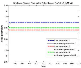
A GARCH(1,1) model, withθ= (α0, α1, β1) = (1,0.3,0.5) and noise process covariance Q = 0.1, is considered. The sample size used is 1000. Similar results are obtained with different initial values.

Figure V shows the nonlinear parameter estimation of GARCH(1,1) model described below.It can be seen the fast convergence of the parameter evolution (see Table 1 for details). For the parameter estimation, it is assumed that the

Figure 1. Nonlinear Parameter Estimation

Figure 2. Nonlinear State 1 Estimation

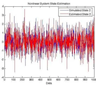
states of the model is always known. As seen in Figures 2 and 3, the simulated states are very close to the estimated states (using the EKF technique), being the Mean Squared Errors 3.2484and0.2332respectively.

Table I

MEAN ANDMEANSQUAREERROR(MSE)OF THE NONLINEAR PARAMETER ESTIMATION

α0 α1 β1

MEAN 0.9817 0.3049 0.5084 MSE 0.0062469 0.00086165 0.0013252

VI. CONCLUSIONS

This work presents for the first time a state space represen-tation for GARCH family of time series models. Moreover,

ISBN: 978-988-18210-6-5

(4)

Figure 3. Nonlinear State 2 Estimation

an efficient numerical method, for nonlinear estimation of GARCH processes, is presented. This procedure is im-plemented using a EKF technique. The numerical results demonstrate the effectiveness of state representation, and shows that it’s appropriate when the objective is to estimate the parameters and the state of a nonlinear system.

ACKNOWLEDGMENT

The authors would like to thank S. Eyheramendy and C. Reyes for many fruitful discussions related to this work.

REFERENCES

[1] I. Berkes, L. Horv´ath and P. Kokoszka, “GARCH processes: structure and estimation,”Bernoulli, vol. 9, no. 2, pp. 201-227, 2003.

[2] T. Bollerslev, “Generalized autoregressive conditional heteroskedastic-ity,”J. Econometrics, vol. 31, no 3, pp. 307-327, 1986.

[3] A. Bose and K. Mukherjee, “Estimating the ARCH parameters by solving linear equations,”J. Time Ser. Anal., vol. 24, no. 2, pp. 127-136, 2003.

[4] J. Durbin and S.J. Koopman, “Time Series Analysis by State Space Methods,”Oxford: Oxford University Press, 2001.

[5] R. Engle, “Autoregressive conditional heteroscedasticity with estimates of the variance of United Kingdom inflation,”Econometrica, vol. 50, no. 4, pp. 987-1007, 1982.

[6] C. Francq and J-M. Zakoian, “Maximum Likelihood Estimation of Pure GARCH and ARMA-GARCH Processes,”Bernoulli vol. 10, pp. 605-637, 2004.

[7] L. Giraitis and P. M. Robinson, “Whittle estimation of arch models,”

Econometric Theory, vol. 17, no. 3, pp. 608-631, 2001.

[8] P. Hall and Q. Yao, “Inference in ARCH and GARCH models with heavy-tailed errors,”Econometrica 71, 285317, 2003.

[9] R.E. Kalman, “A new approach to linear filtering and prediction problems,”Trans ASME J. Basic Eng., 82, 35-45, 1960..

[10] R.E. Kalman and R.S. Bucy, “New results in filtering and prediction theory,”Trans. ASME J. Basic Eng., 83, 95-108, 1961.

[11] D. Kristensen and O. Linton, “A closed-form estimator for the Garch

(1,1)model,”Econometric Theory, vol. 22, no. 2, pp. 323-337, 2006.

[12] E. A. Wan and A. T. Nelson. “Neural dual extended Kalman filtering: applications in speech enhancement and monaural blind signal sepa-ration, ”In Proc. Neural Networks for Signal Processing Workshop. IEEE, 1997.

[13] E. A. Wan, R. van der Merwe, and A. T. Nelson. “Dual Estimation and the Unscented Transformation, ”In S. Solla, T. Leen, and K.-R. Muller, editors, Advances in Neural Information Processing Systems, 12, pp. 666-672. MIT Press, 2000.

[14] A. Weiss, “Asymptotics theory for Arch models: estimation and testing,”Econometric Theory, vol. 2, pp. 107-131, 1986.

ISBN: 978-988-18210-6-5