www.atmos-chem-phys.net/11/8745/2011/ doi:10.5194/acp-11-8745-2011
© Author(s) 2011. CC Attribution 3.0 License.
Chemistry
and Physics
Influences of the variation in inflow to East Asia on surface ozone
over Japan during 1996–2005
S. Chatani and K. Sudo
Graduate School of Environmental Studies, Nagoya University, Nagoya, Japan
Received: 26 August 2010 – Published in Atmos. Chem. Phys. Discuss.: 17 December 2010 Revised: 20 August 2011 – Accepted: 22 August 2011 – Published: 29 August 2011
Abstract.Air quality simulations in which the global chem-ical transport model CHASER and the regional chemchem-ical transport model WRF/chem are coupled have been devel-oped to consider the dynamic transport of chemical species across the boundaries of the domain of the regional chemi-cal transport model. The simulation captures the overall sea-sonal variations of surface ozone, but overestimates its con-centration over Japanese populated areas by approximately 20 ppb from summer to early winter. It is deduced that ozone formation around Northeast China and Japan in summer is overestimated in the simulation. On the other hand, the sim-ulation well reproduces the interannual variability and the long-term trend of observed surface ozone over Japan. Sen-sitivity experiments have been performed to investigate the influence of the variation in inflow to East Asia on the inter-annual variability and the long-term trend of surface ozone over Japan during 1996–2005. The inflow defined in this pa-per includes the recirculation of species with sources within the East Asian region as well as the transport of species with sources out of the East Asian region. Results of sensitivity experiments suggest that inflow to East Asia accounts for ap-proximately 30 % of the increasing trend of surface ozone, whereas it has much less influence on the interannual vari-ability of observed surface ozone compared to meteorologi-cal processes within East Asia.
1 Introduction
Surface ozone is harmful to human health and the ecosys-tem. It causes pulmonary and cardiovascular system effects (WHO, 2006). Damage to vegetation could result in losses of
Correspondence to:S. Chatani
(chatani.satoru@f.mbox.nagoya-u.ac.jp)
agricultural crop yields (Wang and Mauzerall, 2004). In ad-dition to its critical role as an air pollutant, ozone is also one of short-lived climate forcers. Tropospheric ozone radiative forcing has been estimated to be the third largest among var-ious greenhouse agents since pre-industrial times (Forster et al., 2007). Damage to crops and forests could also alter their capabilities to absorb CO2, and indirectly exert changes in
carbon dioxide concentration in the atmosphere (Sitch et al., 2007). Therefore, it is beneficial both to preventing air pollu-tion and to mitigating the climate change to control ambient surface ozone concentration.
In Japan, the environmental quality standard (EQS) has been set for ambient photochemical oxidants which are dom-inated by ozone. However, the achievement rate of EQS for photochemical oxidants has remained almost zero through-out Japan. In fact, the concentration of photochemical oxi-dants is gradually increasing, whereas NOxand non-methane
affected the increasing trend of surface ozone over Japan. Yoshikado (2004) analyzed meteorological conditions and discussed their possible links to increasing surface ozone. Chatani et al. (2011) implied that surface ozone is increasing over the Tokyo metropolitan area because titration of ambient ozone by NO emissions is being suppressed due to stringent NOxemission controls.
Because the atmospheric lifetime of ozone near surface is one to two weeks in summer and one to two months in winter, ambient ozone produced in a polluted region of one continent can be transported to another continent (Akimoto, 2003). Vingarzan (2004) indicated that concentration of background ozone over the mid-latitudes in the northern hemisphere has continued to increase. This increase may have affected the increasing trend of surface ozone over Japan. Thus, the pur-pose of this study is to investigate the influence of the varia-tion in inflow to East Asia on the interannual variability and the long-term trend of surface ozone over Japan during 1996– 2005 through air quality simulation in which global and re-gional chemical transport models (CTMs) are coupled. The target domain of a regional CTM covers the East Asian coun-tries. The influence of the spatial and temporal variation in the regional CTM’s boundary concentrations provided from a global CTM on surface ozone over Japan was investigated. Global CTMs have been applied to investigate the influ-ence of hemispheric ozone transport over Japan. For exam-ple, Wild et al. (2004) used the Frontier Research System for the Global Change (FRSGC) version of the University of California, Irvine (UCI), global CTM, and discussed the influence of trans-Eurasian transport on the air quality over Japan. They indicated that European and North American emission sources have contributed to background ozone over Japan. However, one of the shortcomings in using global CTMs is their coarse resolution which is not suitable to rep-resent the urban and regional air quality. This study com-bined a regional CTM with a global CTM in order to rep-resent surface ozone in regional scale in more detail with finer resolution than global CTMs. A few previous studies in Japan (Yamaji et al., 2006, 2008; Kurokawa et al., 2009a) have utilized results of global CTMs as boundary concentra-tions in their regional CTM simulaconcentra-tions. Participating mod-els in Model Intercomparison Study Asia Phase II (MICS-Asia II) also applied boundary concentrations derived from a global CTM (Carmichael et al., 2008). However, these studies did not consider short-term (daily) and long-term (an-nual) variations in their boundary concentrations. This study represented daily and annual variations in boundary ozone concentrations as done by Takigawa et al. (2007). Another feature of this study is the long-term simulation covering ten years with a regional CTM to discuss the past trend of surface ozone over Japan. Kurokawa et al. (2009a) conducted long-term simulation with a regional CTM for twenty-five years during 1981–2005, but only for springtime. Lin et al. (2010) quantified the pollution inflow and outflow over East Asia in detail by using the simulation framework which is
simi-Table 1. Numerical options, modules and data used in the
WRF/Chem simulation.
Meteorology Microphysics WRF Single-Moment
3-class Longwave radiation Rapid Radiative
Transfer Model Shortwave radiation Dudhia
Surface layer MM5 similarity
Land surface Noah Land Surface
Model
Planetary Boundary layer Yonsei University
Cumulus Grell 3d ensemble
cumulus
Analyses data NCEP/NCAR global
reanalysis Grid nudging coefficients 1.0×10⁻⁴
Chemistry Chemical mechanism RADM2
Photolysis Fast-J
Biogenic emissions Guenther Anthropogenic emissions REAS
lar to this study, but only on March 2001. The present study included all seasons for ten years during 1996–2005, and in-vestigated the trend of surface ozone over Japan.
In this study, “inflow to East Asia” is defined as the ozone and other chemical species which are transported across the boundaries of the domain covering the East Asian countries from the outside. Their origins are out of the scope of this study. Precursors emitted in the East Asian countries and ozone produced from them could be transported out of East Asia and contribute to the increase of hemispheric back-ground ozone. Therefore, inflow to East Asia may be af-fected by precursors emitted from the East Asian countries themselves through the hemispheric transport. Even so, its impacts on the interannual variability and the long-term trend of surface ozone over Japan are worthwhile to be investi-gated because preceding studies using regional CTMs could not evaluate them. The long-term simulation in which global and regional CTMs are coupled in this study has enabled us to examine their impacts by taking short-term and long-term variations in the boundary concentrations of a regional CTM into account.
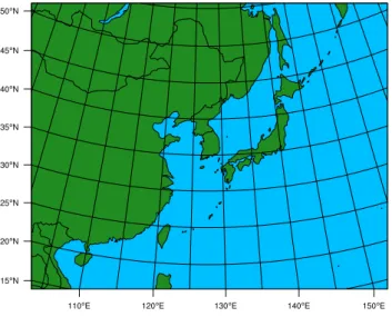
Fig. 1.Target domain of the WRF/chem simulation.
2 Simulation description
2.1 Online-coupled meteorology and chemistry transport model
The online-coupled WRF/chem model (Grell et al., 2005) version 3.0.1.1, in which chemical modules have been incor-porated into the Weather Research and Forecasting (WRF) framework, was used to simulate meteorological field and chemical transport simultaneously. The Community Multi-scale Air Quality modeling system (CMAQ) (Byun and Schere, 2006) has also been widely used to simulate chemi-cal transport. However, several studies (e.g. Lin et al., 2009; Lam and Fu, 2009) reported that artificial downward trans-port of ozone from the lower stratosphere causes overesti-mation of surface ozone when results of global CTMs are directly used as boundary concentrations in CMAQ simula-tions. This problem is more evident when vertical layers are collapsed in CMAQ simulations to alleviate computational costs. One possible reason may be decoupled treatment of vertical transport in meteorology models and CMAQ. On the other hand, the online-coupled WRF/chem uses the same structure of vertical layers and the same numerical scheme for meteorology and chemical transport. This study chose WRF/chem because it is expected to represent vertical trans-port of chemical species in a manner more consistent with meteorology.
Figure 1 shows the target domain of the WRF/chem simu-lation. It covers East Asian countries including Japan, South Korea, North Korea, Taiwan, Mongolia and a large part of China. The horizontal coordinate is based on the Lambert conformal, and the center of the domain is located at latitude 36.0 North and longitude 127.5 East. Grid size is 54×54 km,
and the number of grids is 100×80. The vertical coordinate is
based on the sigma-p coordinate. Model top is 5047 Pa, and
the number of layers is 25. The first six layers are within 2 km above the surface. The lowest layer height is about 70 m, and the layer height around the tropopause is about 1 km. All layer heights are coincided with the global CTM simulation. Ozone in the lowest layer is defined as “surface ozone” in this study.
Numerical options, modules and data used in the WRF/chem simulation are listed in Table 1. National Cen-ters for Environmental Prediction (NCEP)/National Center for Atmospheric Research (NCAR) global reanalysis data (Kistler et al., 2001) were used for the initial condition, the boundary condition, and grid nudging. REAS version 1.11 (Ohara et al., 2007) was used for anthropogenic emissions in Asian countries in each year during 1996–2005. Temporal variations within a year were not provided. Biogenic emis-sions were estimated within the model by using the simple biogenic emission scheme (Guenther et al., 1994). Biomass burning emissions were not considered in this study to avoid large variations in simulated ozone which may be caused by their uncertainties. The chemical mechanism used in the model was Regional Acid Deposition Model (RADM) 2 (Stockwell et al., 1990). All emissions and boundary con-centrations were speciated to RADM2 species groups. The target period of the simulation was ten consecutive years dur-ing 1996–2005.
2.2 Boundary concentrations
Boundary concentrations for the WRF/chem simulation were provided from the global chemical transport model CHASER (Sudo et al., 2002). Details of the CHASER simulation se-tups have been described elsewhere (Sudo et al., 2002; Sudo et al., 2007). Horizontal resolution is T42 (2.8×2.8 degree),
number of vertical layers is 32 from the surface to 40 km, and NCEP/NCAR global reanalysis data (Kistler et al., 2001) were used in the CHASER simulation. Input emissions in each year during 1996–2005 were derived by interpolating or extrapolating the global emission database EDGAR-HYDE 1.4 (Van Aardenne et al., 2001; Olivier and Berdowski, 2001) and EDGAR 32FT2000 (Olivier et al., 2005); Emissions for the US and Asia after 2000 were harmonized with the trend data reported by the US EPA (2007), US EPA (2006), and the REAS emission inventory (Ohara et al., 2007).
Simulated daily concentration of ozone and monthly con-centrations of other chemical species in CHASER grids were interpolated to boundary grids of the WRF/chem domain. Other studies (Kurokawa et al., 2009a; Lin et al., 2009; Lam and Fu, 2009) applied corrections to ozone concentrations in global CTM results, especially in the lower stratosphere when they were used as boundary concentrations in regional CTMs. To the contrary, this study applied no corrections, and utilized all results of the CHASER simulation including the lower stratosphere.
Monitoring stations in populated area
EANET monitoring stations Monitoring sites in China
Fig. 2.Location maps of monitoring stations in populated area, EANET monitoring stations in Japan, and monitoring sites in China which
were used in this study.
were conducted in this study. Boundary concentrations for each year were used in the BXX case. On the other hand, boundary concentrations for the year 2000 were commonly used for all the simulated years in the B00 case. Differences of simulation results between the BXX and B00 cases corre-spond to the influence of the variation in inflow to East Asia in each year from 2000 onwards.
2.3 Observation data
Annual and monthly pollutant concentrations observed at monitoring stations operated by Japanese and local govern-ments are available on the website (National Institute for En-vironmental Studies, 2010). It contains the monitoring data since 1970, which are valuable to evaluate the long-term trends of pollutant concentrations in Japan. The increasing trend of surface ozone in Japan has been reported annually by the Japanese government based on this database (Ministry of the Environment, 2010). Therefore, observation data at 1045 monitoring stations which continued monitoring for photo-chemical oxidants during 1996–2005 was used in this study. Most of the monitoring stations are located in coastal popu-lated areas in Japan as shown in the left map of Fig. 2 because they are operated mainly to evaluate the attainment of EQSs. This database has compiled surface ozone concentration as a daytime average and maximum concentrations of photo-chemical oxidants. Daytime corresponds to fifteen hours from 05:00 a.m. to 08:00 p.m. LT. Strictly speaking, photo-chemical oxidants include other trace oxidants like H2O2and
PAN, but instruments which detect only ozone have been of-ficially approved by the Japanese government because differ-ences in concentrations of photochemical oxidants and ozone are expected to be small. They have been used at some of the monitoring stations. Therefore, differences in concentrations between ozone and photochemical oxidants were ignored in this study. Observed and simulated daytime average concen-trations of surface ozone over Japanese populated areas (av-eraged over 1045 monitoring stations) are mainly discussed in this study.
Additionally, the Acid Deposition Monitoring Network in East Asia (EANET) operates monitoring stations located mainly in remote areas. Observed concentrations of sur-face ozone at ten EANET monitoring stations in Japan were used to validate the performance of the simulation in Japanese background areas during 2000–2005. The loca-tions of EANET monitoring staloca-tions are shown in the middle map of Fig. 2. They are scattered in remote areas throughout Japan. A few studies have reported long-term variations of observed surface ozone in China. The concentrations of sur-face ozone observed at Hok Tsui (Wang et al., 2009), Linan (Xu et al., 2008), and Shangdianzi (Lin et al., 2008) were used to validate the performance of the simulation in China during 1996–2005. Their locations are shown in the right map of Fig. 2.
3 Performance of the simulation
3.1 Horizontal distribution of surface ozone
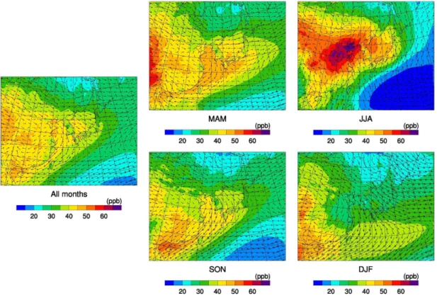
Fig. 3.Horizontal distributions of simulated yearly and seasonal surface ozone and wind fields averaged during 1996–2005 in BXX case.
To the contrary, a high concentration zone is located over northeast China and spreads to Japan. Between high and low concentration zones, the gradient of concentration is steep over Japan. In SON, distributions of surface ozone and wind fields are similar to those in spring, but have slightly different characteristics. Winds from Northeastern China to South-ern China are more evident, and the concentration of sur-face ozone is higher in Southern China and lower in North-ern China than in spring. In DJF, Japan is mostly affected by the transport of cleaner air with northwesterly winds from the Siberian high-pressure system. In addition, titration of am-bient ozone by NO emissions in the cold stagnant air causes low concentration of surface ozone over coastal populated areas.
Other studies have reported similar features in distribu-tions of simulated surface ozone. Kurokawa et al. (2009a) in-dicated that a high concentration zone spreads over Northern China and Japan in the distribution of simulated springtime boundary layer ozone. Difference in concentration over the land and the ocean is not obvious in their distribution pre-sumably because they showed boundary layer ozone which is defined as from the surface to an altitude of 1 km whereas this study discusses only surface ozone. Lin et al. (2009) indicated a high concentration zone concentrated on North-eastern China in the distribution of their simulated ozone for June 2001. Zhu et al. (2004) also indicated that a band of high ozone appears between 35◦N–45◦N and 70◦E–130◦E
in the summertime in their distribution of simulated ozone. The distributions of surface ozone obtained in this study are analogous to those.
3.2 Monthly variation of surface ozone over Japanese populated area
0 10 20 30 40 50 60 70 80
1 7 1 7 1 7 1 7 1 7 1 7 1 7 1 7 1 7 1 7
O3
or
O
x
(
ppb)
Observation (Daytime only) WRF/chem BXX (Daytime only)
WRF/chem BXX (Whole hours) CHASER (Whole hours)
1996 1997 1998 1999 2000 2001 2002 2003 2004 2005
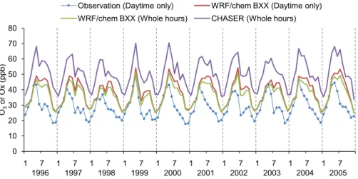
Fig. 4.Observed and simulated concentration of surface ozone over Japanese populated areas in each month during 1996–2005.
0 10 20 30 40 50 60 70
J F M A M J J A S O N D
O3
or
O
x
(
ppb)
Observation (Daytime only) WRF/Chem BXX (Daytime only) WRF/Chem BXX (Whole hours) CHASER (Whole hours)
Fig. 5. Monthly variations of observed and simulated
concentra-tions of surface ozone averaged during 1996–2005 over Japanese populated areas.
Figure 5 shows monthly variations of concentrations of observed and simulated surface ozone averaged during 1996–2005 over Japanese populated areas. The perfor-mance of the WRF/chem simulation from January to April is good. Concentrations of both observed and simulated sur-face ozone are the highest in May. However, the decrease of simulated surface ozone from May is not enough, and over-estimation continues until December. This tendency is more evident in WRF/chem than CHASER. Therefore, ozone for-mation and/or transport on a regional scale may be overesti-mated in summer and autumn.
3.3 Monthly variation of surface ozone in Japanese background area
Figure 6 shows monthly variations of concentrations of ob-served and simulated surface ozone in the BXX case aver-aged during 2000–2005 at each of ten EANET monitoring stations. Absolute values of concentrations are comparable but seasonal variations are different between observed and simulated surface ozone. Concentration of observed surface ozone is the highest in spring and the lowest in summer at all stations. Second peaks in autumn are found at most of stations. The simulation reproduced dips in summer at Oga-sawara and Hedomisaki, which are located in southern is-lands. They indicate that the simulation has capabilities to re-produce background surface ozone which is mainly affected by the inflow to East Asia. However, dips in summer do not appear in simulated values at remaining stations to which the flow passes over the Asian continent and/or Japanese islands. Therefore, overestimation of surface ozone in summer is a problem not only in populated areas but also in most of the background areas except for southern islands in Japan. 3.4 Monthly variation of surface ozone in China
0 20 40 60 80
1 3 5 7 9 11
O3 (ppb) Rishiri 0 20 40 60 80
1 3 5 7 9 11
O3 (ppb) Tappi 0 20 40 60 80
1 3 5 7 9 11
O3 (ppb) Ogasawara 0 20 40 60 80
1 3 5 7 9 11
O3 (ppb) Sado 0 20 40 60 80
1 3 5 7 9 11
O3 (ppb) Happo 0 20 40 60 80
1 3 5 7 9 11
O3 (ppb) Ijirako 0 20 40 60 80
1 3 5 7 9 11
O3 (ppb) Oki 0 20 40 60 80
1 3 5 7 9 11
O3 (ppb) Banryuko 0 20 40 60 80
1 3 5 7 9 11
O3 (ppb) Yusuhara 0 20 40 60 80
1 3 5 7 9 11
O3
(ppb)
Hedomisaki
Observation WRF/Chem CHASER
Fig. 6.Monthly variations of observed and simulated concentrations of surface ozone in the BXX case averaged during 2000–2005 at each
of ten EANET monitoring stations.
0 20 40 60 80
1 3 5 7 9 11 O3 (ppb) Hok Tsui (1994-2007) 0 20 40 60 80
1 3 5 7 9 11 O3 (ppb) Linan (1991-2006) 0 20 40 60 80
1 3 5 7 9 11 O3
(ppb)
Shangdianzi (2004-2006)
Observation WRF/Chem CHASER
Fig. 7. Monthly variations of observed and simulated
concentra-tions of surface ozone in the BXX case averaged during 1996–2005 at each of three monitoring sites in China. The durations of the monitoring are also shown.
concentration zone shown in Fig. 3. Therefore, the concen-tration of surface ozone in a high concenconcen-tration zone located over northeast China may be too emphasized in the simula-tion.
3.5 Discussions on the performance of the simulation
Overall, the simulation used in this study captured the gen-eral seasonal variation of surface ozone. Absolute val-ues of the surface ozone concentration were also repro-duced well at background sites except for summer. How-ever, it turned out that overestimation of surface ozone in summer is a major problem in the simulation used in this study. Other simulation studies also faced overestimation of ozone in summer over East Asia. For example, Holloway et al. (2007) indicated that the global atmospheric chemistry model MOZART tends to overpredict monthly concentra-tions of surface ozone over Japan except in springtime. Ac-cordingly, Lin et al. (2009) reduced boundary concentrations of ozone derived from MOZART results up to 40 % in sum-mer, and conducted regional simulation with WRF-CMAQ. The concentration of simulated ozone became closer to the
observed values, but dips in summer could not be fully re-produced. They concluded that systematic overprediction of summertime O3is due to model inability to accurately
simu-late cloud cover and monsoon rainfall and inadequate repre-sentation of southwesterly/southeasterly inflow of marine air masses.
As shown in Fig. 3, the gradient of surface ozone is steep over Japan in JJA between a high concentration zone around Northeast China and a low concentration zone over the Pa-cific Ocean. The average concentration of simulated surface ozone over Japan in JJA appears to be influenced by trans-port from both zones. The concentration of simulated surface ozone in a high concentration zone is significantly overesti-mated as discussed in Sect. 3.4. Therefore, the contribution of the transport of ozone from a high concentration zone to the average concentration of surface ozone over Japan may be overestimated in summer. Although the simulation cur-rently reproduced dips in summer only at two EANET mon-itoring stations located in the southern islands, dips in sum-mer should be reproduced in more regions over Japan if the relative strength of the influence of a high concentration zone becomes less over Japan.
What are possible reasons for the overestimation of ozone over Northeast China? One of these is uncertainties em-bedded in the emission inventory. Kurokawa et al. (2009b) conducted the adjoint inverse modeling of NOx emissions
using satellite observations of NO2 vertical column
densi-ties. They implied that original NOx emissions of REAS
may be overestimated in July 1996 and 1999 in the East-ern China region, and especially in the Beijing region where NOxemissions in 2002 may also be overestimated. In
-2.5 -2 -1.5 -1 -0.5 0 0.5 1 1.5 2 2.5
1996 1997 1998 1999 2000 2001 2002 2003 2004 2005 O3 anom al y ( ppb) Year Observation BXX B00 All months R=0.73, p=0.017 -6 -4 -2 0 2 4
1996 1997 1998 1999 2000 2001 2002 2003 2004 2005
O3 anom al y ( ppb) Year MAM R=0.74, p=0.013 -8 -6 -4 -2 0 2 4 6 8
1996 1997 1998 1999 2000 2001 2002 2003 2004 2005
O3 anom al y ( ppb) Year JJA R=0.81, p=0.004 -4 -3 -2 -1 0 1 2 3
1996 1997 1998 1999 2000 2001 2002 2003 2004 2005
O3 anom al y ( ppb) Year SON R=0.68, p=0.032 -1.5-2
-1 -0.5 0 0.5 1 1.5 2
1996 1997 1998 1999 2000 2001 2002 2003 2004 2005
O3 anom al y ( ppb) Year DJF R=0.32, p=0.404
Fig. 8.Yearly and seasonal anomalies of observed and simulated daytime average concentrations of surface ozone in BXX and B00 cases
over Japanese populated areas. The correlation coefficients and thep-values between observed and simulated surface ozone are also shown.
OH and HO2 concentrations. They implied the existence
of a pathway which amplifies the degradation of pollutants without producing ozone. Such a pathway is not included in the chemical mechanisms which have been incorporated in current CTMs. The uncertainties illustrated above may lead to overestimated ozone formation in summer over Northeast China.
The resolution of WRF/chem in this study may not be enough to resolve the situation over Japanese populated ar-eas. Chatani et al. (2011) indicated that the much finer reso-lution of the order of 4×4 km can reduce the overestimation
of surface ozone over the Tokyo metropolitan area. Monthly and hourly variations in emissions considered in their simu-lation may also be effective to reduce the overestimation.
4 The Influence of the variation in inflow on the interannual variability of surface ozone
In this section, the influence of the variation in inflow to East Asia on the interannual variability of surface ozone over Japan is discussed. Figure 8 shows anomalies of day-time average concentrations of observed and simulated sur-face ozone in the BXX and B00 cases for all months and each season over Japanese populated areas. Anomalies were calculated as differences of surface ozone concentrations in each year from those averaged during 1996–2005. The av-eraged concentrations in the BXX case were applied to cal-culate anomalies in the B00 case. DJF includes December of the previous year, and the value in 1996 was not calcu-lated. The correlation coefficients and the p values between observed and simulated surface ozone in the BXX case are also shown in figures.
The anomaly of observed surface ozone for all months dips in 1998, and continues to rise from 2002 to 2005. Except for dips in 1999 and 2003, the anomaly of simulated sur-face ozone for all months followed the trend of the observed anomaly. The anomalies of observed surface ozone for each
season were also well reproduced by the simulation except for DJF. The simulation has the capability to reproduce the interannual variability of surface ozone over Japan well, even if it has difficulty reproducing concentration levels in some seasons as discussed in the previous section. The high cor-relation coefficients and low p values between observed and simulated surface ozone also support the good performance of the simulation for the interannual variability of surface ozone except for DJF. Differences of anomalies of simulated surface ozone between the BXX and B00 cases are much smaller than the range of interannual variability. Therefore, it appears that the meteorological processes within East Asia mainly cause the interannual variability of surface ozone over Japanese populated areas and the variation in inflow to East Asia is not a major contributor to it.
Here, causes of the interannual variability of surface ozone over Japan were briefly examined by selecting typical years in which anomalies were large. 2005 in MAM, JJA and SON, and 2004 in DJF were defined as “High” years, and 1998 in MAM, 1999 in JJA, 2000 in SON and 2005 in DJF were de-fined as “Low” years. The distribution of simulated surface ozone and wind fields in “High” and “Low” years, and those of differences in simulated surface ozone and wind fields be-tween “High” and “Low” years in MAM, JJA, SON, and DJF in the BXX case are shown in Fig. 9.
Fig. 9. Distributions of surface ozone and wind fields in “High” years(a), “Low” years(b), and those of differences in surface ozone and wind fields between “High” and “Low” years(c)in MAM, JJA, SON, and DJF in BXX case.
Different characteristics are found in the distribution of surface ozone in other seasons. In JJA, a high concentra-tion zone expands over the Japan Sea in “High” years, and the highest difference between “High” and “Low” years ap-pears there. The air over the Japan Sea is mostly affected by southerly winds in “Low” years, but westerly components of winds are found in “High” years. In SON, the highest difference over Japan appears in Northern Japan where west-erly winds from the continent are more obvious in “High” years. In DJF, positive anomalies appear in most of the
do-main. Northerly winds which transport cleaner air seem to be weaker in “High” years.
-2.5 -2 -1.5 -1 -0.5 0 0.5 1 1.5 2 2.5
1996 1997 1998 1999 2000 2001 2002 2003 2004 2005 O3 anom al y ( ppb) Year Observation BXX BXX-B00 All months (Inflow to East Asia) -3 -2 -1 0 1 2 3
1996 1997 1998 1999 2000 2001 2002 2003 2004 2005
O3 anom al y ( ppb) Year MAM -3 -2 -1 0 1 2 3
1996 1997 1998 1999 2000 2001 2002 2003 2004 2005
O3 anom al y ( ppb) Year JJA -3 -2 -1 0 1 2 3
1996 1997 1998 1999 2000 2001 2002 2003 2004 2005
O3 anom al y ( ppb) Year SON -3 -2 -1 0 1 2 3
1996 1997 1998 1999 2000 2001 2002 2003 2004 2005
O3 anom al y ( ppb) Year DJF
Fig. 10. Yearly and seasonal anomalies of observed and simulated daytime average concentrations of surface ozone in BXX case, and
differences in anomalies between BXX and B00 cases (shown as BXX-B00) over Japanese populated areas. Each value is represented by a marker, and regression lines are drawn.
although other physical and chemical processes may also contribute to the interannual variability. Differences in wind fields may be linked to ENSO in other seasons as well as spring as discussed by Kurokawa et al. (2009a), but they are not in the scope of this study.
5 The influence of the variation in inflow on the long-term trend of surface ozone
In this section, the influence of the variation in inflow to East Asia on the long-term trend of surface ozone over Japan is discussed. Figure 10 shows anomalies of daytime average concentrations of observed and simulated surface ozone in the BXX case for all months and each season over Japanese populated areas. It also shows differences in anomalies be-tween the BXX and B00 cases which correspond to the influ-ence of the variation in modeled inflow. Each value is repre-sented by a marker and regression lines which are expected to reduce the influence of the interannual variability are drawn. Values of observed and simulated surface ozone in the BXX case for all months in 1998 are exceptionally low as shown in Fig. 10. They may be affected by the strongest ENSO event of the century (Chandra et al., 1998). Therefore, values in 1998 were not included to obtain regression lines because they are not appropriate for discussing the long-term trend.
Regression lines of anomalies of observed surface ozone have positive slopes for all months and each season except for DJF. They indicate that observed surface ozone over Japanese populated areas has an increasing trend in most seasons. Regression lines of anomalies of surface ozone simulated in the BXX case almost coincide with those of observed values for all months, MAM and JJA. The simu-lation performs well when reproducing the long-term trend
as well as the interannual variability of surface ozone over Japanese populated areas. The regression lines of differences in anomalies of simulated surface ozone between the BXX and B00 cases also have positive slopes for all months and all seasons. This implies that the variation in inflow to East Asia has influenced to some extent the long-term increasing trend of surface ozone over Japanese populated areas.
Slopes of regression lines are defined as increasing rates of surface ozone here. Figure 11 shows the increasing rates of observed and simulated surface ozone in the BXX case over Japanese populated areas for all months and each season. In-creasing rates of differences in simulated surface ozone be-tween the BXX and B00 cases are included. The range of the increasing rates for BXX-B00 in the 95 % confidence limit, and thep-values below 0.05 are also shown. The
in-creasing rates of observed and simulated surface ozone in the BXX case for all months are 0.18 and 0.15 ppb yr−1,
respec-tively. The corresponding increasing rate of differences in simulated surface ozone between the BXX and B00 cases is 0.06 ppb yr−1. Thus, approximately 30 % of the increasing
trend of surface ozone over Japanese populated area may be contributed by inflow to East Asia. This finding is statisti-cally robust because the p values are low.
0.18 (P=0.04)
0.12
0.40
0.18
-0.04
0.15
0.18
0.40
0.04
0.05
0.06 (P=0.01)
0.04
0.05 (P=0.002)
0.04
0.12 (P=0.03)
-0.1 0 0.1 0.2 0.3 0.4 0.5 0.6 All
months
MAM
JJA
SON
DJF
Increasing rate (ppb/year) Obs.
BXX
BXX-B00 (Inflow to East Asia)
Fig. 11.Increasing rates of observed and simulated concentrations
of surface ozone for all months and each season over Japanese pop-ulated areas in BXX case. Increasing rates of differences in simu-lated concentrations of surface ozone between BXX and B00 cases (represented as BXX-B00) are included. The range of the increas-ing rates for BXX-B00 in the 95 % confidence limit, and thep -values below 0.05 are also shown.
less active and ozone is transported over longer distances be-fore it is removed from the atmosphere.
The increasing rates of simulated surface ozone in the BXX case and differences in simulated surface ozone be-tween the BXX and B00 cases were also calculated for the entire domain. Their distributions with average wind fields during 1996–2005 for all months and each season are shown in Fig. 12. The increasing rates of differences in simulated surface ozone between the BXX and B00 cases for all months are positive nearly throughout the entire domain. They im-ply that inflow to East Asia has contributed to the increasing trend of surface ozone all over East Asia. Although increas-ing rates in DJF are dominant over those for all months be-cause both distributions of increasing rates are similar, higher positive increasing rates which are found close to the bound-aries in distributions in other seasons certainly reach Japan along the major wind direction.
The increasing rates of simulated surface ozone in the BXX case are also positive throughout most parts of the domain. However, their distribution appears different from that of differences in simulated surface ozone between the BXX and B00 cases. It seems that the spatial differences in the increasing trend of surface ozone are caused by fac-tors within the domain. Increasing rates of simulated sur-face ozone in the BXX case are the highest around South-ern China. This region tends to be affected by the transport from coastal populated areas in Eastern and Southern China. In addition, the warmer weather causes active photochemi-cal formation of ozone for longer periods than in Northern China. Wang et al. (2009) reported a high increasing rate of ozone, 0.58 ppb yr−1, during 1994–2007 in Hong Kong,
which matches a value obtained from simulation results.
The distribution of increasing rates of simulated surface ozone in the BXX case for each season is affected by the timescale of photochemical reactions. In JJA, increasing rates are high in regions adjacent to populated areas due to rapid photochemical reactions. In MAM and SON, higher increasing rates spread from the continent to Japan. To the contrary, negative values spread from the continent to Japan in DJF. It seems that increasing NOxemissions in populated
areas cause the negative trends in downwind regions due to titration, and subsequently cause the positive trend over the Pacific Ocean in DJF.
It is noteworthy that higher increasing rates are mainly found in regions downwind from populated areas. Therefore, the increasing trend of surface ozone is affected not only by increasing precursor emissions and inflow to East Asia but also by meteorological fields within East Asia. If there are any long-term variations in meteorological fields, they may also exert influence on the increasing trend of surface ozone. Further studies are necessary to identify the influence of me-teorological fields within East Asia on the increasing trend of surface ozone.
6 Summary
Air quality simulations in which the global chemical trans-port model CHASER and the regional chemical transtrans-port model WRF/chem are coupled have been developed to con-sider the dynamic transport of chemical species across the boundaries of the domain of the regional chemical transport model. The simulation reproduced periodical variation of ob-served surface ozone over Japan, but the concentration of sur-face ozone was overestimated from summer to early winter. This implied that excessive ozone formation around North-east China is one possible reason for overestimation of sur-face ozone over Japan. Further studies are needed to clarify the reasons for this overestimation and to reduce uncertain-ties in precursor emissions and photochemical reactions over East Asia.
The influence of inflow to East Asia was greater in winter, when photochemical reactions are less active.
Kurokawa et al. (2009a) stated that the increasing trend of boundary layer ozone was caused by the recent increase of anthropogenic precursor emissions in East Asia and espe-cially in China. However, it is not possible to attribute all of the remaining 70 % of the increasing trend of surface ozone over Japanese populated areas only to increasing emissions in East Asia. Further studies are required to distinguish the influence of various factors including meteorological condi-tions and titration of ambient ozone by decreasing NO emis-sions as well as increasing emisemis-sions in East Asia. If remain-ing parts of the increasremain-ing trend of surface ozone is attributed to multiple factors, it can be said that the influence of inflow to East Asia is one of dominant factors causing the increas-ing trend of surface ozone over Japanese populated areas. In order to evaluate its impacts, the simulations in which a re-gional CTM is coupled with a global CTM are essential.
Sudo et al. (2007) indicated that ozone exports from boundary layer in China and Asian free troposphere are dis-cerned through much of the Northern Hemisphere, suggest-ing significant and extensive impacts of eastern Asian pollu-tion. Therefore, inflow to East Asia may be largely affected by precursors emitted from the East Asian countries them-selves through the hemispheric transport. Further studies are necessary to identify the origins of inflow to East Asia.
Several modeling studies suggested that background ozone will continue to increase in the future (Dentener et al., 2006). It will certainly influence the future trend of surface ozone over Japanese populated areas. Contributions to the in-ternational cooperation aiming at preserving the global atmo-sphere are essential, not least to improve the local air quality. They should be also beneficial to mitigating the hemispheric transport of pollutants and the climate change.
Acknowledgements. NCEP/NCAR global reanalysis data are from
the Research Data Archive (RDA) which is maintained by the Com-putational and Information Systems Laboratory (CISL) at NCAR. NCAR is sponsored by the National Science Foundation (NSF). The original data are available from the RDA (http://dss.ucar.edu) in dataset number ds090.0. Observation data at monitoring stations operated by Japanese and local governments were obtained from the Environmental Numerical Databases provided by National Institute for Environmental Studies. Observation data at EANET monitoring stations were obtained from the CD-ROM titled “EANET Data Sets on the Acid Deposition in the East Asian Region” provided by the Network Center for EANET.
This research was supported by the Global Environment Research Fund (S-7 and A-0902) by the Ministry of the Environment (MOE), Japan.
Edited by: P. Haynes
References
Akimoto, H.: Global Air Quality and Pollution, Science, 302, 1716–1719, 2003.
Byun, D. W. and Schere, K. L.: Review of the governing equations, computational algorithms, and other components of the Models-3 Community Multiscale Air Quality (CMAQ) modeling system overview, Appl. Mech. Rev., 59, 51–77, 2006.
Carmichael, G. R., Sakurai, T., Streets, D., Hozumi, Y., Ueda, H., Park, S. U., Fung, C., Han, Z., Kajino, M., Engardt, M., Bennet, C., Hayami, H., Sartelet, K., Holloway, T., Wang, Z., Kannari, A., Fu, J., Matsuda, K., Thongboonchoo, N., and Amann, M.: MICS-Asia II: The model intercomparison study for Asia Phase II methodology and overview of findings, Atmos. Environ., 42, 3468–3490, 2008.
Chandra, S., Ziemke, J. R., Min, W., and Read, W. G.: Effects of 1997–1998 El Nino on tropospheric ozone and water vapor, Geo-phys. Res. Lett., 25, 3867–3870, 1998.
Chatani, S., Morikawa, T., Nakatsuka, S., Matsunaga, S., and Mi-noura H.: Development of a framework for a high-resolution, three-dimensional regional air quality simulation and its applica-tion to predicting future air quality over Japan, Atmos. Environ., 45, 1383–1393, 2011.
Dentener, F., Stevenson, D., Ellingsen, K., Van Noije, T., Schultz, M., Amann, M., Atherton, C., Bell, N., Bergmann, D., Bey, I., Bouwman, L., Butler, T., Cofala, J., Collins, B., Drevet, J., Do-herty, R., Eickhout, B., Eskes, H., Fiore, A., Gauss, M., Hauglus-taine, D., Horowitz, L., Isaksen, I. S. A., Josse, B., Lawrence, M., Krol, M., Lamarque, J. F., Montanaro, V., Muller, J. F., Peuch, V. H., Pitari, G., Pyle, J., Rast, S., Rodriguez, J., Sanderson, M., Savage, N. H., Shindell, D., Strahan, S., Szopa, S., Sudo, K., Vandingenen, R., Wild, O., and Zeng, G.: The global atmo-spheric environment for the next generation, Environ. Sci. Tech-nol., 40, 3586–3594, 2006.
Forster, P., Ramaswamy, V., Artaxo, P., Berntsen, T., Betts, R., Fa-hey, D. W., Haywood, J., Lean, J., Lowe, D. C., Myhre, G., Nganga, J., Prinn, R., Raga, G., Schulz, M., and Van Dorland, R.: Changes in Atmospheric Constituents and in Radiative Forcing, in: Climate Change 2007: The Physical Science Basis. Contribu-tion of Working Group I to the Fourth Assessment Report of the Intergovernmental Panel on Climate Change, Cambridge Univer-sity Press, Cambridge, UK and New York, NY, USA, 2007. Guenther, A., Zimmerman, P., and Wildermuth, M.: Natural volatile
organic compound emission rate estimates for U.S. woodland landscapes, Atmos. Environ., 28, 1197–1210, 1994.
Grell, G. A., Peckham, S. E., Schmitz, R., McKeen, S. A., Frost, G., Skamarock, W. C., and Eder, B.: Fully coupled “online” chem-istry within the WRF model, Atmos. Environ., 39, 6957–6975, 2005.
Hofzumahaus, A., Rohrer, F., Lu, K., Bohn, B., Brauers, T., Chang, C.-C., Fuchs, H., Holland, F., Kita, K., Kondo, Y., Li, X., Lou, S., Shao, M., Zeng, L., Wahner, A., and Zhang, Y.: Amplified Trace Gas Removal in the Troposphere, Science, 324, 1702– 1704, 2009.
2007.
Kistler, R., Kalnay, E., Collins, W., Saha, S., White, G., Woollen, J., Chelliah, M., Ebisuzaki, W., Kanamitsu, M., Kousky, V., van den Dool, H., Jenne, R., and Fiorino, M.: The NCEP-NCAR 50-Year Reanalysis: Monthly Means CD-ROM and Documentation, B. Am. Meteorol. Soc., 82, 247–267, 2001.
Kurokawa, J., Ohara, T., Uno, I., Hayasaki, M., and Tanimoto, H.: Influence of meteorological variability on interannual variations of springtime boundary layer ozone over Japan during 1981– 2005, Atmos. Chem. Phys., 9, 6287–6304, doi:10.5194/acp-9-6287-2009, 2009a.
Kurokawa, J., Yumimoto, K., Uno, I., and Ohara, T.: Adjoint in-verse modeling of NOxemissions over eastern China using
satel-lite observations of NO2vertical column densities, Atmos.
Env-iron., 43, 1878–1887, 2009b.
Lam, Y. F. and Fu, J. S.: A novel downscaling technique for the link-age of global and regional air quality modeling, Atmos. Chem. Phys., 9, 9169–9185, doi:10.5194/acp-9-9169-2009, 2009. Lin, M., Holloway, T., Oki, T., Streets, D. G., and Richter, A.:
Multi-scale model analysis of boundary layer ozone over East Asia, Atmos. Chem. Phys., 9, 3277–3301, doi:10.5194/acp-9-3277-2009, 2009.
Lin, M., Holloway, T., Carmichael, G. R., and Fiore, A. M.: Quan-tifying pollution inflow and outflow over East Asia in spring with regional and global models, Atmos. Chem. Phys., 10, 4221– 4239, doi:10.5194/acp-10-4221-2010, 2010.
Lin, W., Xu, X., Zhang, X. and Tang, J.: Contributions of pol-lutants from North China Plain to surface ozone at the Shang-dianzi GAW Station, Atmos. Chem. Phys., 8, 5889–5898, doi:10.5194/acp-8-5889-2008, 2008.
Ministry of the Environment: http://www.env.go.jp/air/osen/index. html (in Japanese), last access: 20 August 2010, 2010.
National Institute for Environmental Studies: http://www.nies.go. jp/igreen/td down.html (in Japanese), 1 June 2010, 2010. Ohara, T., Akimoto, H., Kurokawa, J., Horii, N., Yamaji, K.,
Yan, X., and Hayasaka, T.: An Asian emission inventory of anthropogenic emission sources for the period 1980–2020, At-mos. Chem. Phys., 7, 4419–4444, doi:10.5194/acp-7-4419-2007, 2007.
Olivier, J. G. J. and Berdowski, J. J. M.: Global emissions sources and sinks, in: The Climate System, edited by: Berdowski, J., Guicherit, R. and Heij, B. J., A.A. Balkema Publishers/Swets & Zeitlinger Publishers, Lisse, The Netherlands, 33–78, 2001. Olivier, J. G. J., Van Aardenne, J. A., Dentener, F., Ganzeveld, L.,
and Peters, J. A. H. W.: Recent trends in global greenhouse gas emissions: regional trends and spatial distribution of key sources, in: Non-CO2Greenhouse Gases (NCGG-4), Millpress,
Rotter-dam, 325–330, 2005.
Sitch, S., Cox, P. M., Collins, W. J., and Huntingford, C.: Indirect radiative forcing of climate change through ozone effects on the land-carbon sink, Nature, 448, 791–794, 2007.
Stockwell, W. R., Middleton, P., Chang, J. S., and Tang, X.: The second generation regional acid deposition model chemical mechanism for regional air quality modeling, J. Geophys. Res., 95, 16343–16367, 1990.
Sudo, K., Takahashi, M., Kurokawa, J., and Akimoto, H.: CHASER: A global chemical model of the tropo-sphere 1. Model description, J. Geophys. Res., 107, 4339, doi:10.1029/2001JD001113, 2002.
Sudo, K. and Akimoto, H.: Global source attribution of tropospheric ozone: Long-range transport from vari-ous, source regions, J. Geophys. Res., 112, D12302, doi:10.1029/2006JD007992, 2007.
Takigawa, M., Niwano, M., Akimoto, H., and Takahashi, M.: De-velopment of a One-way Nested Global-regional Air Quality Forecasting Model, SOLA, 3, 81–84, 2007.
Tanimoto, J., Ohara, T., and Uno, I.: Asian anthropogenic emis-sions and decadal trends in springtime tropospheric ozone over Japan: 1998–2007, Geophys. Res. Lett., 36, L23802, doi:10.1029/2009GL041382, 2009.
US EPA: Air emissions summary through 2005, http://www.epa. gov/airtrends/2006/emissions summary 2005.html, last access: 10 July 2010, 2006.
US EPA: Inventory of U.S. greenhouse gas emissions and sinks: 1990–2005, EPA430-R-07-002, 2007.
Van Aardenne, J. A., Dentener, F. J., Olivier, J. G. J., Klein Gold-ewijk, C. G. M., and Lelieveld, J.: A 1×1 degree resolution dataset of historical anthropogenic trace gas emissions for the period 1890–1990, Global Biogeochem. Cy., 15, 909–928, 2001. Vingarzan, R.: A review of surface ozone background levels and
trends, Atmos. Environ., 38, 3431–3442, 2004.
Wang, T., Wei, X. L., Ding, A. J., Poon, C. N., Lam, K. S., Li, Y. S., Chan, L. Y., and Anson, M.: Increasing surface ozone concen-trations in the background atmosphere of Southern China, 1994– 2007, Atmos. Chem. Phys., 9, 6217–6227, doi:10.5194/acp-9-6217-2009, 2009.
Wang, X. and Mauzerall, D. L.: Characterizing distributions of sur-face ozone and its impact on grain production in China, Japan and South Korea: 1990 and 2020, Atmos. Environ., 38, 4383– 4402, 2004.
WHO: Air quality guidelines. Global update 2005. Particulate mat-ter, ozone, nitrogen dioxide and sulfur dioxide, WHO Regional Office for Europe, Copenhagen, Denmark, 2006.
Wild, O., Pochanart, P., and Akimoto, H.: Trans-Eurasian trans-port of ozone and its precursors, J. Geophys. Res., 109, D11302, doi:10.1029/2003JD004501, 2004.
Xu, X., Lin, W., Wang, T., Yan, P., Tang, J., Meng, Z., and Wang, Y.: Long-term trend of surface ozone at a regional background station in eastern China 1991–2006: enhanced variability, At-mos. Chem. Phys., 8, 2595–2607, doi:10.5194/acp-8-2595-2008, 2008.
Yamaji, K., Ohara, T., Uno, I., Tanimoto, H., Kurokawa, J., and Akimoto, H.: Analysis of the seasonal variation of ozone in the boundary layer in East Asia using the Community Multi-scale Air Quality model: What controls surface ozone levels over Japan?, Atmos. Environ., 40, 1856–1868, 2006.
Yamaji, K., Ohara, T., Uno, I., Kurokawa, J., Pochanart, P., and Akimoto, H.: Future prediction of surface ozone over east Asia using models-3 community multiscale air quality modeling sys-tem and regional emission inventory in Asia, J. Geophys. Res., D08306, doi:10.1029/2007JD008663, 2008.
Yoshikado, H.: One possible factor causing recent trend of pho-tochemical oxidants, Journal of Japan Society for Atmospheric Environment, (in Japanese), 39, 188–199, 2004.