A multi-model assessment of pollution transport to the Arctic

(1)

www.atmos-chem-phys.net/8/5353/2008/ © Author(s) 2008. This work is distributed under the Creative Commons Attribution 3.0 License.

Chemistry

and Physics

A multi-model assessment of pollution transport to the Arctic

D. T. Shindell1, M. Chin2, F. Dentener3, R. M. Doherty4, G. Faluvegi1, A. M. Fiore5, P. Hess6, D. M. Koch1,

I. A. MacKenzie4, M. G. Sanderson7, M. G. Schultz8, M. Schulz9, D. S. Stevenson4, H. Teich1, C. Textor9, O. Wild10, D. J. Bergmann11, I. Bey12, H. Bian13, C. Cuvelier3, B. N. Duncan13, G. Folberth12, L. W. Horowitz5, J. Jonson14, J. W. Kaminski15, E. Marmer3, R. Park16, K. J. Pringle7,*, S. Schroeder8, S. Szopa9, T. Takemura17, G. Zeng18, T. J. Keating19, and A. Zuber20

1_{NASA Goddard Institute for Space Studies and Columbia University, New York, NY, USA} 2_{NASA Goddard Space Flight Center, Greenbelt, MD, USA}

3_{European Commission, Institute for Environment and Sustainability, Joint Research Centre, Ispra, Italy} 4_{School of GeoSciences, University of Edinburgh, UK}

5_{NOAA Geophysical Fluid Dynamics Laboratory, Princeton, NJ, USA} 6_{National Center for Atmospheric Research, Boulder, CO, USA} 7_{Met Office Hadley Centre, Exeter, UK}

*_{now at: Max Planck Institute for Chemistry, Mainz, Germany} 8_{ICG-2, Forschungszentrum-J¨ulich, Germany}

9_{Laboratoire des Science du Climat et de l’Environnement, Gif-sur-Yvette, France} 10_{Department of Environmental Science, Lancaster University, UK}

11_{Atmospheric Science Division, Lawrence Livermore National Laboratory, CA, USA}

12_{Laboratoire de Modélisation de la Chimie Atmosphérique, Ecole Polytechnique Fédérale de Lausanne, Lausanne,}

Switzerland

13_{Goddard Earth Science & Technology Center, U. Maryland Baltimore County, MD, USA} 14_{Norwegian Meteorological Institute, Oslo, Norway}

15_{Center for Research in Earth and Space Science, York University, Canada}

16_{Atmospheric Chemistry Modeling Group, Harvard University, Cambridge, MA, USA and School of Earth and}

Environmental Sciences, Seoul National University, Seoul, Korea

17_{Research Institute for Applied Mechanics, Kyushu University, Japan}

18_{National Centre for Atmospheric Science, Department of Chemistry, University of Cambridge, Cambridge, UK} 19_{Office of Policy Analysis and Review, Environmental Protection Agency, Washington DC, USA}

20_{Environment Directorate General, European Commission, Brussels, Belgium}

Received: 28 March 2008 – Published in Atmos. Chem. Phys. Discuss.: 6 May 2008 Revised: 5 August 2008 – Accepted: 15 August 2008 – Published: 10 September 2008

Abstract.We examine the response of Arctic gas and aerosol concentrations to perturbations in pollutant emissions from Europe, East and South Asia, and North America using re-sults from a coordinated model intercomparison. These sen-sitivities to regional emissions (mixing ratio change per unit emission) vary widely across models and species. Intermodel differences are systematic, however, so that the relative im-portance of different regions is robust. North America con-tributes the most to Arctic ozone pollution. For aerosols

Correspondence to:D. T. Shindell (dshindell@giss.nasa.gov)

(2)

Euro-pean emissions. Model diversity for aerosols is especially large, resulting primarily from differences in aerosol physi-cal and chemiphysi-cal processing (including removal). Compari-son of modeled aerosol concentrations with observations in-dicates problems in the models, and perhaps, interpretation of the measurements. For gas phase pollutants such as CO and O3, which are relatively well-simulated, the processes

contributing most to uncertainties depend on the source re-gion and altitude examined. Uncertainties in the Arctic sur-face CO response to emissions perturbations are dominated by emissions for East Asian sources, while uncertainties in transport, emissions, and oxidation are comparable for Euro-pean and North American sources. At higher levels, model-to-model variations in transport and oxidation are most im-portant. Differences in photochemistry appear to play the largest role in the intermodel variations in Arctic ozone sen-sitivity, though transport also contributes substantially in the mid-troposphere.

1 Introduction

Transport of pollution to the Arctic affects both air quality and climate change. While levels of pollutants such as tro-pospheric ozone and aerosols are generally lower in the Arc-tic than in industrialized areas, they can have substantial im-pacts on climate. For example, aerosols can greatly perturb the Arctic radiation balance (Garrett and Zhao, 2006; Lubin and Vogelmann, 2006). Though pollutant levels outside the Arctic may in fact have a larger influence than local pollutant levels on Arctic climate (Shindell, 2007), at least for histor-ical changes, it is important to understand the sources of the pollution that reaches the Arctic. This pollution alters local radiative fluxes, temperature profiles and cloud properties. Pollutant levels within the Arctic are especially important for climate in the case of black carbon (BC), which clearly has a strong local climate impact when it is deposited onto snow and ice surfaces, reducing their albedo (Hansen and Nazarenko, 2004; Jacobson, 2004; Warren and Wiscombe, 1980; Vogelmann et al., 1988).

While air pollution in most heavily populated areas of the world comes predominantly from local and regional emis-sions, pollution in the remote Arctic is primarily a result of long-range transport from source regions outside the Arc-tic. Pollution can be transported to the Arctic along a va-riety of pathways, with transport at low levels followed by uplift or diabatic cooling and tranport at high altitudes fol-lowing uplift near the emission source regions seen in a Lan-grangian model (Stohl, 2006). While there is general support for large contributions to Arctic pollution from both Eurasian and North American emissions (Xie et al., 1999; Sharma et al., 2006), it is crucial to quantify the relative importance of emissions from various source regions in determining local pollutant levels (Stohl, 2006). This will enable us to better

understand the influence of past emission changes, such as the apparent maximum in North American BC emissions in the early 20th century (McConnell et al., 2007), and future changes such as the expected continuing decrease in sions from mid/high latitude developed nations while emis-sions from lower latitude developing nations increase. Ad-ditionally, it will help to inform potential strategies to miti-gate Arctic warming via short-lived pollutants (Quinn et al., 2007).

In this paper, we examine model simulations performed within the Task Force on Hemispheric Transport of Air Pol-lution (HTAP), a project to develop a fuller understanding of long-range transport of air pollution in support of the 51-nation Convention on Long-Range Transboundary Air Pol-lution. Using these simulations, we can analyze transport of a variety of idealized and actual pollutants to the Arctic in a large suite of models, allowing us to characterize the rel-ative importance of emissions from different source regions as well as uncertainties in current understanding. As it is dif-ficult to determine the source regions for Arctic pollutants directly from observations, and there have been some appar-ent inconsistencies in previous modeling studies (Law and Stohl, 2007), we believe that examining results from a large suite of models is a useful endeavor.

2 Description of simulations and analyses

A series of simulations were designed to explore source-receptor relationships (i.e. the contribution of emissions from one region, the source, to concentrations or deposition in a receptor region). The source regions were chosen to en-compass the bulk of Northern Hemisphere emissions: Eu-rope (EU: 10 W–50 E, 25 N–65 N, which also includes North Africa), North America (NA: 125 W–60 W, 15 N–55 N), East Asia (EA: 95 E–160 E, 15 N–50 N) and South Asia (SA: 50 E–95 E, 5 N–35 N) (Fig. 1). Northern Asia (Russia) was not included as a source region as its total emissions of most pollutants are comparatively small (at least for anthropogenic sources). However, given their proximity to the Arctic, emis-sions from this area can contribute substantially to Arctic pollution and so we caution that our analyses are not exhaus-tive. We define the Arctic poleward of 68 N as our recep-tor region. A base case simulation was initially performed using each model’s own present-day emissions. Additional simulations then explored the response to a 20% reduction of anthropogenic emissions of nitrogen oxides (NOx) alone,

(3)

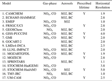
Table 1.Models simulations used in the analyses.

Model Gas-phase Aerosols Prescribed Horizontal lifetime Resolution

1. CAMCHEM NOx, CO SO2, BC Y 1.9

2. ECHAM5-HAMMOZ SO2, BC 2.8

3. EMEP NOx, CO SO2 1.0

4. FRSGC/UCI NOx, CO Y 2.8

5. GEOSChem NOx SO2, BC 2.0

6. GISS-PUCCINI NOx, CO SO2, BC Y 4.0

7. GMI NOx, CO SO2, BC Y 2.0

8. GOCART-2 SO2, BC 2.0

9. LMDz4-INCA SO2, BC 2.5

10. LLNL-IMPACT NOx, CO SO2, BC 2.0

11. MOZARTGFDL NOx, CO SO2, BC Y 1.9

12. MOZECH NOx, CO Y 2.8

13. SPRINTARS SO2, BC 1.1

14. STOCHEM-HadGEM1 NOx, CO 3.8

15. STOCHEM-HadAM3 NOx, CO SO2 Y 5.0

16. TM5-JRC NOx SO2, BC 1.0

17. UM-CAM NOx, CO Y 2.5

The response to perturbations in emissions of the indicated species were simulated by the models listing those species. Prescribed lifetime indicates that an additional simulation with idealized pre-scribed lifetime tracers was also performed. Note that a few models did not perform all the regional perturbation experiments. Horizon-tal resolution is in degrees latitude.

As models used different base case anthropogenic emis-sions, the 20% perturbations differed in absolute amounts. Hence we generally analyze changes in Arctic abundances normalized by the regional emissions change between the control and the perturbation using direct emissions (CO, BC) or the dominant precursor (sulfur dioxide (SO2) for sulfate

(SO4), NOxfor ozone (O3)). Hereafter we refer to this

quan-tity, in mixing ratio per Tg emission per season or year, as the Arctic sensitivity to source region emissions. With the excep-tion of non-linearities in the response, this separates out the effect of intermodel differences in emissions. Uncertainties in emissions are of a different character than the physical un-certainties that we also explore, as the former depend on the inventories used to drive models while the latter are intrinsic to the models themselves.

The response to emissions changes in all four HTAP source regions were analyzed. All these simulations included a minimum of 6 months integration prior to analysis to allow for stabilization, followed by a year of integration with 2001 meteorology (2001 was chosen to facilitate planned compar-isons with campaign data for that year). Differences in me-teorology were present, however, as models were driven by data from several reanalysis centers, or in some cases mete-orology was internally-generated based on prescribed 2001 ocean surface conditions. Additionally, some models directly prescribed meteorology while others used linear relaxation towards meteorological fields. Note that the North Atlantic Oscillation index was weakly negative during 2001, while the broader Arctic Oscillation index showed a stronger nega-tive value during winter, with weak posinega-tive values for most

Arctic

North

America

Europe

East

Asia

South

Asia

Fig. 1.The Arctic and the four source regions (shaded) used in this study.

of the remainder of the year. These indicies are reflective of the strength of the Northern Hemisphere westerly winds, with weaker winds associated with reduced transport to the Arctic (Eckhardt et al., 2003; Duncan and Bey, 2004; Sharma et al., 2006).

Idealized tracer simulations were also performed to iso-late the effects of intermodel differences in transport from other factors affecting trace species distributions. For these simulations, all models used identical emissions of a CO-like tracer with a prescribed globally uniform lifetime of 50 days. A second tracer (“soluble CO”) used the same emis-sions and lifetime, but was subjected to wet deposition as applied to sulfate. Three additional tracers used identical anthropogenic volatile organic compound (VOC) emissions and had prescribed lifetimes of 5.6, 13 and 64 days. The range of model results in these simulations (other than the soluble tracer) thus reflects only the variation in the trans-port algorithms used and in the meteorology used to drive the transport (which differed among models as discussed above). Emissions from different source regions were tagged for the CO-like and soluble CO tracers (but not for the VOC-like tracers). We examine the Arctic concentration of the re-gionally tagged tracer divided by the source region emission, analogous to the Arctic sensitivity described above (though these are absolute concentrations in a single run rather than a difference between a control and a perturbation run).

(4)

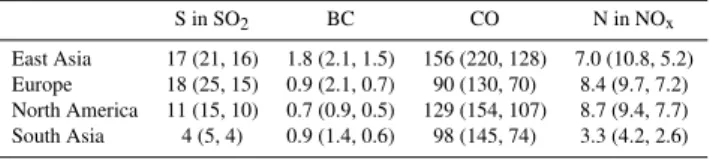
Table 2.Mean (max, min) of total emissions in each region in Tg/yr across all models in their base run.

S in SO2 BC CO N in NOx

East Asia 17 (21, 16) 1.8 (2.1, 1.5) 156 (220, 128) 7.0 (10.8, 5.2) Europe 18 (25, 15) 0.9 (2.1, 0.7) 90 (130, 70) 8.4 (9.7, 7.2) North America 11 (15, 10) 0.7 (0.9, 0.5) 129 (154, 107) 8.7 (9.4, 7.7) South Asia 4 (5, 4) 0.9 (1.4, 0.6) 98 (145, 74) 3.3 (4.2, 2.6)

NOx=NO+NO2

those in the lowest model layer. The global mean pressure of this layer varies from 939 to 998 hPa across models (though different representations of topography could lead to larger variations at some points), suggesting that for most locations differences in definition of the surfacew layer will contribute only minimally to intermodel variations. Values at 500 and 250 hPa levels are interpolated from model output. All sea-sons refer to their boreal timing.

3 Modeled sensitivities, concentrations and deposition

In this section, we first consider Arctic sensitivities and con-centrations in the idealized simulations using the passive tracer with a prescribed 50 day lifetime for which regional emissions were tagged (Sect. 3.1). We then analyze similar quantities for both gases and aerosols in the simulations us-ing realistic chemistry and physics (Sect. 3.2). Finally, we investigate model results for the deposition of black carbon to the Arctic (Sect. 3.3).

3.1 Prescribed lifetime tracer

Transport of European emissions to the Arctic surface is clearly largest in winter (Fig. 2) based on results for the CO-like 50-day lifetime tracer from 8 models (Table 1). During all seasons, the Arctic surface level is most sensitive to Eu-ropean emissions (Fig. 2). In the middle troposphere, the sensitivities to emissions from Europe and North America are usually comparable, sensitivities to East Asian emissions are somewhat less, and sensitivities to South Asian emissions are quite small outside of summer (probably because of the greater distance to the Arctic from this region, Fig. 1). These results are consistent with the “polar dome” or “polar front” that impedes low-level transport from relatively warm and humid areas such as North America and East Asia into the Arctic during the cold months while allowing such transport at higher altitudes from those regions and at low-levels from Eurasia, which often lies within the polar dome (Law and Stohl, 2007; Klonecki et al., 2003; Stohl, 2006). During summer, when the polar front is at its furthest north, emis-sions from all four source regions have a comparable influ-ence on the Arctic surface (per unit emission), with a slightly larger contribution from Europe.

In the upper troposphere, the models tend to show compa-rable sensitivities for all four regions. The spread of model results is typically similar to that seen at lower levels. Sensi-tivities in the upper troposphere are greatest in summer for all regions, consistent with the surface for Asian emissions but opposite to the surface seasonality seen for European emis-sions. The largest sensitivities in the upper troposphere are to summertime Asian emissions.

3.2 Active gas and aerosol species

We now investigate the more realistic, but more complex, full gas and aerosol chemistry simulations. We sample only the models that performed the perturbation runs for a particular species (Table 1). The divergence in model results in the con-trol run is extremely large in the Arctic. For example, annual mean CO varies by roughly a factor of 2–3 at all levels ex-amined. Arctic sulfate varies across models by factors of 8 at the surface, 600 in the mid-troposphere, and 3000 in the upper troposphere. Though some models clearly must have unrealistic simulations, we purposefully do not exclude any models at this stage as our analysis attempts to identify the sources of this enormous divergence among models. We note that the diversity of model results in the Arctic is not terribly different from that seen elsewhere. Examining annual means using equally sized areas over the US and the tropical Pa-cific, polluted and remote regions, respectively, we find CO variations of roughly a factor of 2 across models, and stan-dard deviations at various altitudes are 14–22% of the mean in those regions, only slightly less than the 22–29% in the Arctic. For sulfate, the range and standard deviation across models are smaller at the surface for the US, where they are a factor of 6 and 36% (versus Arctic values of a factor of 8 and 52%), but greater for the remote Pacific, where they are a factor of 40 and 62%. At higher levels, the range is only slightly less than that seen in the Arctic, and standard devi-ations are 86–124% of the mean in the other regions, also similar to the 98–99% seen in the Arctic.

We first examine the total contribution from each source region to the annual average gas or aerosol amount in the Arctic. This includes the influence of variations in emission inventories among the models (Table 2). These variations are quite large, often as great as a factor of two between min-imum and maxmin-imum. The range of SO2and BC emissions

used in the models is especially large for Europe compared to other regions, probably because of rapid changes with time and the many estimates that have been made for European emissions. For the multimodel mean, we find that at the surface, European emissions dominate the Arctic abundance of sulfate and BC, and to a lesser extent CO (Table 3 and Fig. 3). Arctic surface ozone responds most strongly to NOx

(5)

al-ppbv/Tg per season

DJF MAM JJA SON

Surface 500 hPa 250 hPa

DJF MAM JJA SON DJF MAM JJA SON

0 .2 .4 .6 .8

0 .1 .2 .3 .4

0 .1 .2 .25

.15

.05 East Asia

Europe North America South Asia

Fig. 2. Arctic sensitivity at three levels for the seasonal average CO-like tracer in terms of mixing ratio per unit emission from the given source region in the prescribed 50-day lifetime tracer simulations (8 models). Boxes show the central 50% of results with the median indicated by the horizontal line within the box, while the bars indicate the full range of model sensitivities.

Table 3.Annual average Arctic absolute mixing ratio decreases due to 20% reductions in anthropogenic emissions in each region.

EA EU NA SA

Surface

Sulfate (pptm) 2.16±1.92 (13%)1.87 (13%) 12.4±9.8 (73%) 10.0 (71%) 2.27±1.97 (13%) 2.03 (15%) 0.20±0.23 (1%) 0.09 (1%) BC (pptm) 0.18±0.22 (17%) 0.10 (16%) 0.77±0.75 (72%) 0.47 (74%) 0.11±0.11 (10%) 0.05 (8%) 0.01±0.02 (1%) 0.01 (2%) CO (ppbv) 2.23±1.07 (26%) 1.8 (24%) 3.35±1.12 (39%) 2.84 (37%) 2.42±0.75 (29%) 2.42 (32%) 0.51±0.15 (6%) 0.51 (7%) Ozone (ppbv) 0.12±0.04 (27%) 0.11 (24%) 0.11±0.07 (24%) 0.13 (28%) 0.19±0.07 (42%) 0.20 (43%) 0.02±0.01 (7%) 0.02 (4%) 500 hPa

Sulfate (pptm) 11.4±10.4 (25%) 10.6 (25%) 23.3±20.3 (51%) 22.9 (53%) 9.83±9.09 (21%) 9.16 (21%) 1.32±1.78 (3%) 0.53 (1%) BC (pptm) 0.91±0.95 (38%) 0.75 (43%) 0.97±0.99 (41%) 0.68 (39%) 0.41±0.41 (17%) 0.26 (15%) 0.10±0.13 (4%) 0.05 (3%) CO (ppbv) 2.38±1.01 (31%) 1.88 (26%) 2.20±0.54 (28%) 2.11 (30%) 2.52±0.71 (33%) 2.43 (34%) 0.61±0.17 (8%) 0.68 (10%) Ozone (ppbv) 0.26±0.09 (23%) 0.24 (22%) 0.35±0.11 (31%) 0.39 (36%) 0.44±0.15 (40%) 0.40 (37%) 0.07±0.05 (6%) 0.05 (5%) 250 hPa

Sulfate (pptm) 17.4±16.4 (36%) 15.6 (41%) 14.6±14.1 (30%) 11.8 (31%) 11.3±11.6 (24%) 7.93 (21%) 4.68±5.38 (10%) 2.42 (7%) BC (pptm) 1.16±1.08 (48%) 0.75 (47%) 0.45±0.40 (18%) 0.34 (21%) 0.36±0.33 (15%) 0.23 (15%) 0.47±0.50 (19%) 0.27 (17%) CO (ppbv) 1.35±0.48 (36%) 1.28 (35%) 0.77±0.21 (20%) 0.70 (19%) 1.11±0.28 (29%) 1.14 (31%) 0.58±0.23 (16%) 0.57 (15%) Ozone (ppbv) 0.22±0.01 (25%) 0.21 (25%) 0.22±0.17 (25%) 0.18 (22%) 0.35±0.19 (39%) 0.35 (42%) 0.10±0.07 (11%) 0.09 (11%)

For each species, values are multi-model means and standard deviations, followed by medians. The percentage of the total from these four source regions for each individual region is given in parentheses for both mean and median values. Ozone and sulfate changes are in response to NOxand SO2emissions changes, respectively.

most as large as that from Europe for BC. By the upper tro-posphere, both total sulfate and BC show the largest impact from East Asian emissions, especially for BC (Fig. 3). The amount of CO from each region also undergoes a shift with altitude, as European emissions become steadily less impor-tant relative to East Asian and North American emissions. The relative importance of regional NOxemission changes to

Arctic ozone is less dependent upon altitude, with the largest contribution from North America at all levels. The results are consistent looking at either the multi-model mean or me-dian values. These are generally quite similar for CO and ozone, while the median is typically lower than the mean for the aerosols, but the relative importance of different regions is almost unchanged between these two statistics (Table 3).

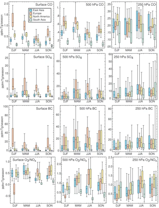
We next turn to Arctic sensitivities (Arctic concentration change per unit source region emission change, hence re-moving the influence of emission inventory variations across

models) rather than total Arctic concentrations, first examin-ing seasonal sensitivities for CO, SO4, and BC (Fig. 4). The

(6)

BC Sulfate

CO Ozone

Surface 250 hPa

Fig. 3.Relative importance of different regions to annual mean Arctic concentration at the surface and in the upper troposphere (250 hPa) for the indicated species. Values are calculated from simulations of the response to 20% reduction in anthropogenic emissions of precursors from each region (using NOxfor ozone). Arrow width is proportional to the multimodel mean percentage contribution from each region to

the total from these four source regions (as in Table 3).

Examining the CO sensitivity to the emissions with the greatest impact (EU, NA and EA), the range of annual aver-age values is roughly a factor of 2–3 among the 11 models. The standard deviation is much smaller (∼20–30%), indi-cating that most models are relatively consistent. The sea-sonality of the Arctic CO sensitivity depends on the source region. At the surface, the multimodel mean sensitivity to European emissions clearly maximizes in winter, while for North American and especially East Asian emissions the maximum sensitivity is in spring. These two regions also differ in their seasonality, however, with the minimum sen-sitivity in fall for East Asian emissions but in summer for North American emissions.

For surface sulfate, Arctic sensitivities in individual mod-els vary greatly. For the annual average, the range spans 2.8 to 17.4 pptm/(Tg S)/season. (Note that the annual average values are in units of pptm/Tg/season for comparison with seasonal sensitivities. Values in pptm/Tg/year are1_/₄_{of these}

season numbers).

Interestingly, the models separate into two groups: of the 13 models, 6 have annual average sensitivities below 4 pptm/(Tg S)/season, while the other 7 have sensitivities of 7.2–17.4 pptm/(Tg S)/season. Seasonal surface sensitivities show an even larger spread (Fig. 4). Median sensitivities to European emissions are comparable in all seasons though the spread in the central 50% of models is greatest in winter and spring. Sulfate sensitivities to East Asian and North Amer-ican emissions maximize in spring, as for CO. In the mid-troposphere, sensitivities are generally largest for European emissions, while in the upper troposphere they are greatest for South Asian emissions in spring and East Asian emis-sions during other seasons.

(7)

ppbv/Tg/season

Surface CO 500 hPa CO 250 hPa CO

Surface BC 500 hPa BC 250 hPa BC

pptm/Tg/season

Surface SO4 500 hPa SO4 250 hPa SO4

ppbv/Tg/season

Surface O3/NOx 500 hPa O3/NOx 250 hPa O3/NOx

.05 .10 .15 .20 .25 .30 .35

.2 .4 .6 .8 1.

0 0.5 1.0 1.6 2.0

DJF MAM JJA SON

0 10 20 30 40 50 60

0 20 40 60

0 5 10 15 20 25

0.5 1.0 1.5 2.0 2.5

0.0 0.5 1.0 1.5 2.0

-0.5 0.0 0.5 1.0

DJF MAM JJA SON DJF MAM JJA SON

DJF MAM JJA SON DJF MAM JJA SON DJF MAM JJA SON

East Asia Europe North America South Asia

0 20 40 60 80

0 20 40 60

pptm/Tg/season

0 20 40 60 80 100

Fig. 4.Arctic sensitivity to emissions from the given region for seasonal averages of CO, sulfate, BC and ozone mixing ratios at the indicated heights. Sensitivities are the difference between the simulation perturbing a given emission and the control, normalized by the emissions change in the species (CO, BC) or its primary precursor (S in SO2for SO4, N in NOxfor O3)in the indicated source region. Symbols as in

Fig. 2. Note change in vertical scale between columns.

to European emissions during the other seasons (means of 9–17 pptm/(Tg C)/season). The enhanced winter sensitivity results from both faster transport during winter and slower removal at this time as the Arctic is stable and dry (Law and Stohl, 2007). During spring, summer and fall, the mid-troposphere, like the surface, is most sensitive to European BC emissions. During winter, however, sensitivity to North American and European emissions is almost identical. Inter-estingly, the seasonality of sensitivity can vary with altitude: the sensitivity of surface BC to European emissions is great-est in winter, while the sensitivity of mid-tropospheric BC to

(8)

Greenland Arctic

(except Greenland)

DJF MAM JJA SON

m

-2 x 10

-17

m

-2 x 10

-17

0 50 100 150

0 20 40 60 80 100 120

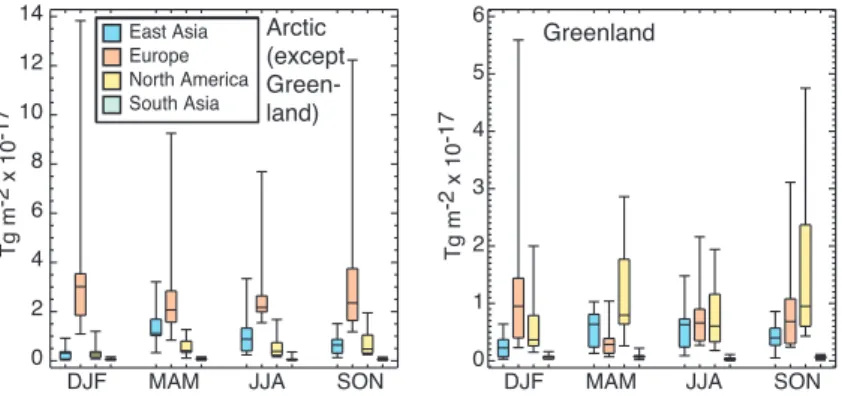
Fig. 5.Sensitivity of Arctic-wide (left, excluding Greenland) and Greenland (right) BC deposition to regional emissions (Tg deposition per Tg emission per unit area per season). Values are calculated from the 20% anthropogenic emissions perturbation simulations.

The sensitivity of Arctic surface ozone to source region NOx emissions is quite different than that for the other

species examined here (Fig. 4). Note that MOZECH and UM-CAM were excluded from the O3/NOxanalysis due to

imbalances in their nitrogen budget diagnostics. Sensitivity to winter European emissions is negative for most models (i.e. reduced NOx emissions leads to more Arctic ozone).

This results from direct reaction of NOxwith ozone in the

relatively dark conditions that much of the high-latitude Eu-ropean emissions encounter. The cancellation of negative winter and positive non-winter ozone sensitivities leads to a lower annual average European influence on Arctic sur-face ozone than for other species (Table 3). Spring sursur-face ozone concentrations show comparable sensitivities to East Asian, European and North American emissions, while sum-mer concentrations are most sensitive to European and fall to European and North American emissions. During winter, sensitivities to South Asian emissions are nearly as large as those for East Asian and North American emissions. Sensi-tivities in the mid-troposphere show a similar pattern to those seen at the surface (Fig. 4). The upper troposphere shows comparable sensitivities for all four of the source regions, with greatest sensitivity to South Asian emissions in win-ter and spring, though North American emissions have the largest annual average influence (Fig. 3).

The magnitude of the sensitivity increases with altitude for SO4and O3, stays roughly constant for BC, and decreases for

CO. This may reflect the greater removal of soluble aerosols and ozone precursors at low levels relative to insoluble CO. In addition, both SO4and O3are produced photochemically

at higher altitudes, while CO is photochemically removed aloft.

A critical result of the analysis is that for both sensitivities and totals, discrepancies between models are systematic, so that the relative importance of different regions is robust de-spite the large differences among models in the magnitude of the contribution from a particular region. For example, ev-ery participating model finds the largest total contribution to

annual average surface SO4, BC, and CO to be from Europe.

Similarly, all models find that in the upper troposphere, East Asia is the largest annually-averaged source for BC, with all but 3 giving first rank to East Asia for sulfate and CO as well. Looking at annual totals, 9 out of 11 models have a larger contribution to 500 hPa Arctic ozone from North America than from Europe even though the standard deviations over-lap substantially (Table 3). Every model finds that the Arctic sensitivity during winter, fall and spring for surface SO4, BC

and CO is largest for European emissions. This holds even during summer for sulfate and BC, while for CO all but 1 model have the greatest sensitivity to European emissions. 3.3 Arctic deposition of black carbon

In addition to atmospheric concentrations, deposition of BC to the Arctic is of particular interest due to its climate im-pact, as discussed previously. We now explore the relative importance of the various source regions to BC deposition to Greenland and to the rest of the Arctic, and use the multi-model results to characterize the robustness of these results. We examine both the total BC deposited and also the BC de-position sensitivity by calculating the Tg deposited per unit area per Tg source region emission. Deposition is calculated on all surfaces, including open ocean, though albedo will be affected by the flux to snow and ice surfaces.

Deposition of BC to the Arctic (excluding Greenland) is most sensitive to emissions from Europe in every season (Fig. 5), and is generally quite similar to the BC surface mix-ing ratio sensitivity (Sect. 3.2). That sensitivity to European emissions is greatest is clear even though the spread in model sensitivities is very large, a factor of 3 to 5 for European emissions, for example. The large range often results from just one or two models. For example, the deposition sensi-tivities for the Arctic (except Greenland) during summer for European emissions are within 39 to 66 m−2₁₀−17_{in 9}

mod-els, while the remaining model has a value of 154 m−2₁₀−17

(9)

di-Greenland Arctic

(except Green-land)

DJF MAM JJA SON

0 2 4 6 8 10 12 14

Tg m

-2 x 10

-17

0 1 2 3 4 5 6

Tg m

-2 x 10

-17

Fig. 6.Total Arctic-wide (left, excluding Greenland) and Greenland (right) BC deposition (Tg deposition per unit area per season) in response to 20% anthropogenic emission change from each source region.

agnostics). However, even the range within the central 50% of models is substantial in other seasons (Fig. 5). Median sensitivities are largest in fall and winter for European emis-sions, but in spring, summer and fall for North American emissions and in spring for East Asian emissions. Examin-ing the BC deposited per unit BC emitted (i.e. multiplyExamin-ing the values in Fig. 5 by area), the multi-model mean percent-age of emissions that are deposited in the entire Arctic (in-cluding Greenland) is 0.02% for South Asian, 0.10% for East Asian, 0.19% for North American and 0.70% for European emissions.

Deposition of BC to Greenland shows different sensitivi-ties compared with the rest of the Arctic, with the largest re-sponse to North American emissions in non-winter seasons (Fig. 5). This results from the high topography of Green-land, which allows the inflow of air from the relatively warm and moist North American, and to a lesser extent East Asian, source areas to occur more easily there than in the rest of the Arctic (Stohl, 2006).

Examining the total BC deposition response to 20% re-gional emissions changes, we find similar results for the Arctic excluding Greenland as for the sensitivity (compare Figs. 5 and 6). Most significantly, total deposition is greatest from Europe in every season. Again the spread of results is large, but the central 50% of models are distinctly separated for Europe from other regions in all seasons but spring. In that season, East Asian emissions take on greater importance as they are large and the sensitivity to East Asian emissions maximizes in spring (Fig. 5). For the annual average, total deposition to the Arctic outside of Greenland is clearly dom-inated by European emissions (Table 4). We reiterate that emissions from Northern Asia (Russia) were not studied in these analyses.

The change in total deposition to Greenland in response to 20% regional emissions changes is roughly evenly split between the impact of European and North American emis-sions (Fig. 6). Deposition of BC from East Asia is as large or nearly as large as that from these regions in spring and

Table 4. Annual average BC deposition to Greenland and Arctic excluding Greenland (Tg/m2×10−17) due to 20% of anthropogenic emissions from each region.

EA EU NA SA

Greenland

All models 0.5±0.3 0.9±0.8 1.0±0.8 0.06±0.04 Excluding largest 0.4±0.3 0.6±0.3 0.8±0.6 0.05±0.02 Excluding smallest 0.5±0.3 0.9±0.8 1.1±0.9 0.07±0.03

Arctic (excluding Greenland)

All models 0.9±0.5 3.3±2.8 0.5±0.4 0.07±0.05 Excluding largest 0.8±0.5 2.5±1.2 0.5±0.3 0.06±0.03 Excluding smallest 0.9±0.5 3.6±2.8 0.6±0.4 0.08±0.05

Values are multi-model means and standard deviations.

(10)

emis-Alert (83 N, 63 W)

J F M A M J J A S O N D

RMS < 40 ppbv: 1-CAMCHEM 3-EMEP 4-FRSGC/UCI 6-GISS-PUCCINI 7-GMI 11-MOZARTGFDL 12-MOZECH 14-STOCHEM-HadGEM1 17-UM-CAM RMS >=50 ppbv 10-LLNL-IMPACT 15-STOCHEM-HadAM3

Barrow (71 N, 157 W)

J F M A M J J A S O N D 0 50 100 150 200 CO (ppbv)

Summit (73 N, 39 W)

J F M A M J J A S O N D Barrow (71 N, 157 W)

J F M A M J J A S O N D 0 10 20 30 40 50 60 Ozone (ppbv)

Spitsbergen (79 N, 12 E )

0 200 400 600 800 11 8 8 15 1

RMS < 190 pptm 5-GEOSCHEM 6-GISS-PUCCINI 7-GMI 8-GOCART-2 10-LLNL-IMPACT RMS >= 250 pptm 1-CAMCHEM 2-ECHAM5-HAMMOZ 3-EMEP 9-LMDz4-INCA 11-MOZART-GFDL 13-SPRINTARS 15-STOCHEM-HadAM3 16-TM5-JRC

0 200 400 600 800 Sulfate (pptm)

Alert (83 N, 63 W)

J F M A M J J A S O N D 0 20 40 60 80 100 Barrow (71 N, 157 W)

J F M A M J J A S O N D 0 20 40 60 80 BC (pptm) 2 0 50 100 150 200

2, 13, 16

5 8 11 6 10 15 3 3 10 15 6 4 7 11 1 14 15 16 4 7 14 0 10 20 30 40 50 60

Alert (83N, 63W)

10 6 8 1 ₁₅ 6 6 8 6 8 6

Fig. 7.Observed and modeled seasonal cycles of trace species surface concentrations at the indicated Arctic sites. Model results in all panels are in grey. Plots for CO (top row) and ozone (second row) show observations from the NOAA Global Monitoring Division, with 1992-2006 means and standard deviations in red (except for Summit O3, which is 2000–2006) and 2001 in blue. Sulfate plots (third row) show

observations from Alert during 1980-1995 (left) and from the EMEP site in Spitsbergen during 1999-2005 in red, with 2001 Spitsbergen data in blue. BC data (bottom row) are from the IMPROVE site at Barrow during 1996-1998 (red), and from Sharma et al. (2006) for both Barrow and Alert using equivalent BC over 1989-2003 (purple). Models are listed by RMS error scores to the right of each row using the groupings discussed in the text. Models that are separated from others are labeled with the numbers as in the text at right (or Table 1).

sions. Deposition to the Arctic (exclusive of Greenland) is similarly skewed (Table 4) and robust in the regional rank-ings across models. Hence as for atmospheric mixing ratios and concentration sensitivities (Sect. 3.2), the relative contri-bution of emissions from the various source regions to BC deposition can be determined with much higher confidence than the magnitude for any particular region.

4 Comparison with Arctic observations

Observational datasets are quite limited in the Arctic, mak-ing it challengmak-ing to reliably evaluate models in this region. Nevertheless, it is worth investigating how well the models perform and how our results are influenced by any models which appear to be clearly unrealistic in their Arctic

simula-tions. In this section, we compare the modeled and measured seasonal cycles of surface CO, ozone, sulfate and BC for se-lected stations in the Arctic. Root-mean-square (RMS) errors between the monthly mean modeled and observed values are used to evaluate the models, though this is clearly only one possible measure of model/observation agreement. We then evaluate the influence of screening out less realistic models in Sect. 5.

(11)

errors for the two sites of between 17 and 40 ppbv, with the exception of two that have RMS values of 54 and 83 ppbv. We note that no model stands out as substantially better than the others (the model with the second lowest RMS error has a value only 3 ppbv greater than the lowest score). While the EMEP model stands out from the others with clearly larger values during fall (Fig. 7), it is not obviously better or worse in comparison with observations over the full annual cycle. Note also that none of the outlying models (those labeled in Fig. 7) has CO emissions distinctly different from the other models. For example, the two models with greatest RMS errors have global CO emissions of 1115 Tg/yr and Euro-pean emissions of 74 and 111 Tg/yr, both well within the range across all models of 1018–1225 Tg/yr for global and 70-130 Tg/yr for European emissions. Hence excluding the two models with highest RMS error provides a reasonable subset for repeating the CO analyses.

Comparison of ozone observations (based on updates from Oltmans and Levy, 1994) with the models shows that the sim-ulations again have a fairly wide spread. Modeled values are generally reasonable during summer and fall at Barrow, though some models have underestimates, but agreement is poor during winter and spring. Nearly all models underpre-dict ozone at Summit. Those that overestimate ozone at Bar-row during spring often do a better job at Summit, as they fail to capture the large observed springtime contrast between these two sites. This leads to comparable error scores to other models. All models have average RMS errors of 7–12 ppbv except for STOCHEM-HadGEM1 with a value of 21 ppbv. We find that exclusion of a single model, however, does not appreciably change the results presented previously.

For sulfate observations, we use data from the EMEP network’s station on Spitsbergen (Hjellbrekke and Fjæraa, 2007) and data from Alert (Sirois and Barrie, 1999), though the Alert data covers earlier years. The sea-salt compo-nent has been removed from these data. The models gen-erally perform poorly in simulating Arctic sulfate (Fig. 7). Most substantially underestimate Arctic concentrations, by more than an order of magnitude in several models. Many that show annual mean sulfate concentrations of about the right magnitude have seasonal cycles that peak in summer or fall, while the observations show a spring maximum. This leads to RMS error values that are fairly large for all mod-els, with multi-model means of 201 (Alert) and 272 (Spits-bergen) pptm. However, models cluster in two groups, with none having average values for the two sites between 190 and 250. Hence we can test if the subset of models with RMS values below 190 pptm yields a different result than the full suite of models.

Note that comparison with measurements taken from 1996–1999 at Denali National Park (from the Interagency Monitoring of Protected Visual Environments: IMPROVE, http://vista.cira.colostate.edu/improve) at 64◦_{N (just outside} the Arctic region we use here) show similar discrepancies between models and observations. The multi-model mean

RMS error at Denali is 249 pptm. Hence although the com-parison at Alert may be influenced by differing emissions during the 1980s, the overall results suggest that discrepan-cies between models and observations occur throughout the high latitudes. As for CO, there is no clear relationship be-tween the emissions used by the models and their Arctic sim-ulations. For example, SO2 emissions from Europe, which

have the largest influence on the Arctic, are 15–20 Tg S/yr (mean 18 Tg S/yr) in the group of models with lower RMS values, and 8–25 Tg S/yr (mean 16 Tg S/yr) in the high RMS group, of which half the models have emissions within the range seen in the lower RMS group. Given that models also show large diversities over the US, where emissions are more consistent, and since the model-to-model sulfate concentra-tions vary much more than the model-to-model emissions, we believe the cause of the model/measurement discrepan-cies is largely different representations of aerosol chemical and physical processing and removal rather than emissions (see Sect. 5.2).

We also attempted to evaluate the simulation of BC in the models. Comparison with observations from Sharma et al. (2006) suggests that models greatly underpredict BC in the Arctic (Fig. 7). However, the available measurements are in fact equivalent BC (EBC), which is obtained by con-verting light absorbed by particles accumulated on a filter in a ground-based instrument to BC concentrations. Uncer-tainties in the optical properties of BC make this conversion quite challenging. Additionally, other light absorbing species such as OC and especially dust influence the measurements, so the EBC would tend to be high relative to actual BC. This is consistent with the sign of the model/observations differ-ence (Fig. 7), though the other species are expected to have fairly small contributions in the Arctic, and hence a substan-tial underestimate of BC in the models is likely. Models also appear to substantially underestimate BC in comparison with IMPROVE data from Barrow (updated from Bodhaine, 1995), which itself differs significantly from the Sharma et al. (2006) data. The Barrow data is also derived from opti-cal absorption measurements. Given the large apparent dis-crepancies for BC for all models, we conclude that it is not feasible to determine the relative realism of the models using currently available data, though it appears that models with a greater transport of BC to the Arctic are in general more realistic.

5 Causes of intermodel variations

(12)

ppbv/Tg

Transport

13 8

10 8

9 11 11

14

9

7 5 15

ppbv/Tg

26 19

14 14

25 30 16

24

16

24 25₅₀ Transport+CO loss

.10 .20 .30

ppbv 24

41 24

23 46

37

27

27 26

44 Transport+CO loss+Emissions

1 2 3 4 5 6

0 0

24 24

.04 .08 .12

0

Fig. 8.Annual Arctic average carbon monoxide response to source region emissions as a function of processes included in the models. The influence of transport is shown via the Arctic sensitivity in the prescribed 50 day lifetime CO-like tracer runs (left). The influence of transport plus CO oxidation is given by the sensitivity in the full chemistry run (center). The influence of transport plus oxidation plus emissions is also given by the full chemistry run, this time without normalization by the source region emissions change (right). Numerical values over each bar give the fractional variation (standard deviation as a percentage of the mean). Symbols as in Fig. 2.

5.1 Isolating processes governing variations in CO and ozone

We first compare the intermodel variability in Arctic sensitiv-ities in the run with the prescribed lifetime “CO-like” tracer to that with realistic CO. As the two sets of experiments do not use directly comparable CO, we analyze the standard de-viation as a percentage of the mean response (the fractional variation) among models. All models in the analysis per-formed both the prescribed lifetime and full chemistry runs.

The fractional variation of sensitivity is always larger in the full chemistry analyses than in the prescribed 50 day life-time case (numerical values in Fig. 8). The relative size of the fractional variations in the prescribed lifetime and full chem-istry runs depends on the altitude analyzed and the source region. At the Arctic surface, the intermodel fractional vari-ation in the prescribed lifetime runs is 9–14%, roughly two-thirds that seen in the full chemistry runs (16–26%) for all regions (Fig. 8). This indicates that differences in modeled transport to the Arctic play an important role in CO near the surface. In the middle troposphere, transport and chemical oxidation by OH contribute a comparable amount to inter-model differences in Arctic CO, while in the upper tropo-sphere transport plays a much smaller role. At the surface and in the mid-troposphere, adding in the intermodel varia-tion in emissions (i.e. no longer normalizing by emissions) leads to larger fractional variances across the models. This is especially so for East Asia, where including the intermodel variation in emissions nearly triples the fractional variance of the Arctic response at the surface and middle troposphere across models. The effects are smaller for emissions from Europe or North America at these levels, where emissions variations add ∼5–13% to the fractional variance, a com-parable range to that from transport (8–14%) and oxidation (6–11%) variations among models. Emissions uncertainties from South Asia have an even smaller impact than those from Europe or North America, barely changing the frac-tional variance.

Thus the intermodel variation in the influence of source region CO emissions on the Arctic surface and mid-troposphere is dominated by emissions for East Asia, by transport and oxidation for South Asia, and all three terms (transport, oxidation and emissions) play comparable roles for Europe and North America. In the upper troposphere, the intermodel fractional variations are dominated by oxida-tion differences, whose importance gradually increases with altitude. We note, however, that while the 250 hPa inter-model differences are important, the variation across the cen-tral 50% of models in CO sensitivity in the upper troposphere is only∼40%, among the smallest range for any species at any level (Fig. 4).

(13)

a long-lived species such as CO. This is especially true for quality-screened models, in which case fractional variations in the mid and lower troposphere are 22% or less for CO sensitivity to emissions from Europe, and 13% or less for emissions from East Asia or North America.

Though model results are relatively consistent for CO, it is interesting to examine the relationship across models be-tween the Arctic sensitivities and the global mean chemical lifetime (lifetimes for portions of the globe could not be cal-culated using the available diagnostics). A high correlation would indicate that the removal rates of CO (by oxidation) play an important role in intermodel variations in sensitivity. We find that either using all models or the quality-screened subset there is little correlation between CO sensitivity and global mean lifetime for the surface and mid-troposphere, ex-cept for South Asian emissions (Table 5). There is some cor-relation for all regions in the upper troposphere (R20.4–0.7). Hence it appears that the CO chemical lifetime, a measure of the CO oxidation rate, does not play a large role in determin-ing the sensitivity of the Arctic to NA, EU and EA emissions perturbations below the upper troposphere. These results are consistent with the increasing importance with height of oxi-dation seen in the comparison between the prescribed life-time and full chemistry simulations. For emissions from South Asia, which have to travel further to the Arctic, the chemical lifetime does appear to play an important role, es-pecially in the mid and upper troposphere.

Ozone’s response to NOxemissions perturbations can be

of either sign, indicating non-linearities in chemistry that pre-clude explanation via linear correlation analysis between the response and ozone’s lifetime. We can, however examine correlations between Arctic ozone sensitivity and intermodel variations in ozone dry deposition or transport (using the pas-sive tracer simulations for the latter). We find that model-to-model variations in dry deposition account for little of the spread in Arctic ozone sensitivity to NOxperturbations, even

at the surface (R2<0.3 at all levels, <0.1 at surface). Cor-relations between Arctic ozone sensitivity and transport (us-ing the prescribed lifetime tracer values. as in the left panel of Fig. 8, for each model) are similarly weak at the surface and 250 hPa (R2<0.25). In the mid-troposphere (500 hPa), however, correlations are R2=0.4 to 0.5 for NA, EA and SA, indicating that at those levels transport variations account for roughly half the intermodel variation in Arctic ozone sen-sitivity. At other levels, however, it appears that model-to-model differences in the non-linear ozone photochemistry must play the dominant role in the intermodel spread of sen-sitivities. Consistent with this, annual mean ozone sensitiv-ity to NOxperturbations shows a variation across models of

35–80% of the mean across regions and altitudes, which is substantially larger than the 8–15% in the prescribed 50 day lifetime tracer experiments

Table 5. Lifetime or residence time (days) and correlation coef-ficients (R2)between those times and Arctic sensitivity across the models.

EA EU NA SA

CO subset Surface correlation .0 .3 .1 .8

(Global mean 500 hPa correlation .0 .0 .0 .8

lifetime 62±12) 250 hPa correlation .3 .3 .4 .6

CO all Surface correlation .3 .0 .3 .9

(Global mean 500 hPa correlation .4 .2 .3 .9

lifetime 57±15) 250 hPa correlation .4 .4 .5 .5

BC all Mean residence time 4.9±2.0 5.8±1.4 5.1±1.5 6.6±1.5

Surface correlation .8 .8 .8 .2

500 hPa correlation .8 .7 .8 .3

SO₄subset Mean residence time 4.8±0.9 7.0±1.9 4.7±0.9 5.6±1.2

SO4all Mean residence time 4.3±1.9 6.1±2.2 4.7±2.1 5.3±2.5

250 hPa correlation .6 .3 7 .4

Global mean multimodel means and standard deviations of resi-dence times for regional emissions for aerosols and global mean chemical lifetime from the control run for CO are given. R2values are linear correlations between those times and the Arctic sensitivi-ties at the given pressure levels. “All” and “subset” refer to the mod-els used in the analysis (see text for subsets). The EMEP model was excluded since it includes the NH only and hence its global lifetime is not precisely equivalent to the others. In the CO analysis, GMI and MOZECH were not included due to problematic diagnostics.

5.2 Isolating processes governing variations in aerosols We examine the relationship between the Arctic concentra-tions and the aerosol lifetimes, as for CO. For aerosols, how-ever, we are able to calculate the global residence time for regional emissions perturbations. These are determined from the change in burden over the change in removal rates in the regional perturbation experiments. Note that this calculation implicitly assumes that the residence time is the same in the two experiments, which given the relatively small emissions perturbations imposed in our experiments should be a good approximation.

(14)

Table 6.Standard deviations of annual mean Arctic values of pre-scribed lifetime tracers across models (%).

surface 500 hPa 250 hPa

5.6 day VOC 19.7 6.4 14.0

13 day VOC 18.2 5.6 7.9

64 day VOC 9.7 3.9 6.0

50 day CO 7.5 6.9 7.8

50 day soluble CO 62.6 65.7 76.7

The three VOC-like tracers used identical VOC emissions, while the two CO-like tracers used CO emissions. Hence comparison within the VOC subset shows the effect of lifetime changes, comparison of the two CO tracers shows the effect of solubility, and differences between the 64 day VOC and 50 day CO are mostly due to differing emissions locations.

transport of species in the aqueous phase). The role of trans-port that can be identified from the prescribed lifetime tracer simulations also does not include linkages between transport and wet removal that result from removal rates varying with location, such as for wet removal processes that depend on local precipitation. Hence transport has a specific, limited meaning in our analysis.

The range of intermodel variations in Arctic sensitivity is much larger for BC than for CO (Fig. 4). The intermodel variation in residence time for BC among models is roughly a factor of 2 and accounts for most of the spread (Table 5). This variation is much greater than the variation in efficiency of dry transport to the Arctic at most levels from any region as seen in the prescribed lifetime simulations (e.g. Fig. 8), even accounting for the intermodel transport variations be-ing roughly twice as large for a tracer with BC’s lifetime than with CO’s (Table 6). Hence the other factors affecting residence time, including aerosol aging from hydrophobic to hydrophilic and rainout/washout of the aerosols, appear to play important roles in governing the Arctic sensitivity to re-gional BC emissions from middle to higher Northern lati-tudes (EU, NA, and EA). In other words, the large variations in how long BC remains in the global atmosphere seems to be more important in determining how much reaches the Arctic than are dry transport differences or local Arctic removal pro-cesses (which contribute only a minor fraction of the global removal). This result is consistent with the strong sensitivity in the export efficiency of Asian BC to the conversion life-time from hydrophobic to hydrophilic seen in a study based on 2001 aircraft data (Park et al., 2005). For emissions from South Asia, the global annual mean residence time of BC is less closely correlated with the Arctic sensitivity. Hence for emissions from this region, both intermodel variations in BC residence times and in transport appear to be important factors in creating model diversity.

For sulfate, the fractional variation in annual average sen-sitivity to regional emissions across models is∼68–112%,

much greater than that seen in the prescribed 50 day lifetime runs where fractional variations were only∼8–15% (Fig. 8), or the 6–20% variations in the response to global emissions for the 5.6 day lifetime tracer (Table 6) (note that the inter-model variations in reponse to global emissions are 0–50% less than those for regional emissions in the 50 day lifetime experiments). This suggests that for sulfate, variations in large-scale physical and chemical processing of aerosol (re-moval of sulfate and/or SO2, oxidation of SO2, etc.) account

for a major portion of the divergence between models. This is consistent with the order of magnitude increase in model-to-model variations going from insoluble to soluble passive tracers that are otherwise identical (Table 6). When inter-model emissions variations are not removed from the sul-fate response calculations, the annual average fractional vari-ance increases only modestly (∼10%), to 79–120% across the models. Thus emissions differences appear to play a mi-nor role in the model-to-model variations.

(15)

pro-East Asia Europe

North America South Asia

10 20 30 40 50 60 70 80 90

0 2 4 6 8 10 12 14 16 18

Fig. 9.Relative contribution of regional emissions to winter Arctic surface BC. Values are the relative contribution (%) to the total response to emissions from the four source regions (top row), the relative contribution (%) per unit source region emission (middle row), and the standard deviation of the latter across the HTAP models (bottom row). Results are based on 8 models (three models with small-spatial scale structure were excluded from these calculations for clarity).

cesses using additional diagnostics not available in the HTAP archive, and would benefit from additional simulations per-turbing only aerosol precursors.

Overall, the comparison between the prescribed lifetime tracer and full chemistry simulations and the analyses of the correlation between residence times and Arctic concentra-tions both support the conclusion that dry transport differ-ences among the models play a major role in the intermodel variations of insoluble, relatively long-lived CO. They are similarly important contributors to the model-to-model dif-ferences in mid-tropospheric ozone. However, these appear to be less important contributors to the intermodel variations in the Arctic sensitivity to aerosol emissions, for which un-certainties in aerosol physical and chemical processing, in-cluding wet removal, play the largest roles. Variations among models’ Arctic cloud phase (ice versus liquid) and uncer-tainty about removal of aerosol by ice clouds may contribute to the large spread of aerosol results.

We also examined the relationship between horizontal res-olution in the models and their representations of transport and of trace species in general. Horizontal resolution, using latitude, ranges from 1 to 5 degrees. We find R2 correla-tions with resolution (using latitude) to be extremely low for lifetimes and sensitivities. Hence there is no straightforward correlation with resolution.

6 Discussion and conclusions

The spread in model results for Arctic pollutants is very large for both gaseous species and aerosols. Differences in mod-eled transport, chemistry, removal and emissions all con-tribute to this spread, which makes climate and composition projections for the Arctic extremely challenging.

This study has identified the largest contributing factors to the diversity of model results. We have shown that for sul-fate and BC (including deposition of the latter), uncertain-ties in modeling of aerosol physical and chemical process-ing are extremely important, with lesser roles for emissions and for dry transport. Further studies to determine precisely which physical processes play the largest role, such as those suggested by (Textor et al., 2006), would help prioritize re-search. In contrast, for CO, transport and emissions are im-portant drivers of uncertainty in simulating surface responses to source region emissions, while transport, emissions and oxidation rates all play comparable roles at higher altitudes. For ozone, our analysis suggests that transport plays a sub-stantial role in the intermodel variations in sensitivity, but that photochemical differences among the models appear to be the dominant contributor.

(16)

East Asia Europe

North America South Asia

10 20 30 40 50 60 70 80 90

0 2 4 6 8 10 12 14 16 18

Fig. 10.As Figure 9 but for summer.

lesser extent on their (precursor) emissions (Textor et al., 2007). These results held true for both the global aerosol load and the polar (>80◦_{in both hemispheres) fraction. Our} results also suggest that the contribution of intermodel dry transport differences to disparities in Arctic aerosol loading is relatively small, reinforcing the conclusion that aerosol and cloud physical and chemical processing (e.g. removal, oxidation and microphysics) is the principle source of uncer-tainty in modeling the distributions of these species in the Arctic. For realistic species whose lifetimes vary with loca-tion, transport and physical processes are inherently coupled, however, and hence for the soluble aerosols these cannot be easily separated as sources of uncertainty.

For cases in which transport plays a substantial role in in-termodel variability, such as CO or mid-tropospheric ozone, intercomparison among different models driven by the same meteorological fields would help determine the underlying reason for the range of results (complimenting studies of a single model driven by multiple meteorological fields, such as (Liu et al., 2007)). Differences in convection certainly contribute to transport variations among models. Model nu-merical schemes could also play a role, though algorithms such as conservation of second-order moments have been shown to generally transport trace species quite well, pre-serving gradients and not being too diffusive (Prather, 1986). However, this merits further study as many models may use less capable transport schemes. Additionally, the degree of agreement between chemical-transport models driven by of-fline meteorological fields and general circulation models

that are relaxed towards offline meteorological fields remains to be characterized. Our comparison shows no clear effect of horizontal resolution.

Although the intermodel variations in transport to the Arc-tic are large, many of them are systemaArc-tic across models so that differences between sensitivities to emissions from var-ious regions are robust across models. In particular, we find that Arctic surface concentrations of BC, sulfate, and CO are substantially more sensitive to European emissions than to those from other regions. Similar results are obtained for the mid-troposphere (500 hPa), though the difference in sen-sitivities between Europe and other regions is not as large as for the surface. Hence per unit Tg emission change, Eu-ropean emissions are the most important for these species. We expect that Arctic sensitivities to emissions from North-ern Asia would be generally similar to their European coun-terparts given the similarity in proximity and meteorological conditions.

The sensitivity of Arctic surface concentrations to Euro-pean emissions maximizes during winter for CO, sulfate and BC. In the middle troposphere, sensitivity to European emis-sions is greatest in summer for aerosols. Sensitivity to East Asian emissions peaks during spring for BC, sulfate, and CO at both the surface and 500 hPa. Hence the relative impor-tance of emissions from different regions varies seasonally. For surface ozone, Arctic concentrations during summer are most sensitive to European emissions of NOx, but

(17)

Table A1. Arctic average absolute mixing ratio decreases due to 20% reductions in anthropogenic emissions in each region for the four seasons.

Dec–Jan

EA EU NA SA

Surface

Sulfate (pptm) 1.33±1.38 (8%) 14.1±12.4 (80%) 1.90±2.07 (10%) 0.31±0.41 (2%) BC (pptm) 0.12±0.19 (7%) 1.44±1.55 (86%) 0.10±0.12 (6%) 0.02±0.04 (1%) CO (ppbv) 2.22±1.01 (21%) 4.97±2.07 (47%) 2.90±0.75 (27%) 0.56±0.12 (5%) Ozone (ppbv) 0.13±0.05 (26%) 0.14±0.22 (28%) 0.18±0.07 (36%) 0.05±0.02 (10%)

500 hPa

250 hPa

Sulfate (pptm) 10.2±10.5 (38%) 5.23±6.25 (19%) 7.39±9.34 (27%) 4.25±5.62 (16%) BC (pptm) 0.70±0.73 (47%) 0.17±0.18 (11%) 0.24±0.26 (16%) 0.39±0.38 (26%) CO (ppbv) 1.32±0.43 (34%) 0.74±0.25 (19%) 1.19±0.29 (31%) 0.58±0.25 (15%) Ozone (ppbv) 0.16±.10 (26%) 0.12±0.12 (19%) 0.25±0.18 (40%) 0.09±0.06 (15%)

Mar–May

EA EU NA SA

Surface

500 hPa

250 hPa

Jun–Aug

EA EU NA SA

Surface

500 hPa

250 hPa

Sep–Nov

EA EU NA SA

Surface

500 hPa

250 hPa

(18)

American emissions. In the upper troposphere, concentra-tions for all species typically show comparable sensitivity to emissions from all four source regions, though there is a gen-eral tendency for a lower sensitivity to South Asian emissions (especially for CO).

The deposition of BC to the Arctic outside of Greenland is most sensitive to emissions from Europe in all seasons. In contrast, deposition of BC to Greenland is most sensitive to North American emissions, except during winter when sensi-tivity to European emissions becomes comparable. Total de-position of BC, rather than per unit emission, is again greater from Europe than the other regions for the Arctic exclusive of Greenland. Annual mean total BC deposition onto Green-land is greatest from North America and Europe, which are nearly equal, with a substantial but lesser contribution from East Asia. These conclusions are robust across the models examined here. Total deposition to Greenland is primarily due to emissions from North America and East Asia during spring, when Greenland is less affected by European emis-sions than in other seasons. As springtime deposition appears to be especially effective in inducing large snow-albedo feed-backs (Flanner et al., 2007), this suggests an enhanced role in Greenland climatic forcing for East Asian and North Amer-ican emissions relative to their annual mean contribution to deposition.

The recent recovery of ice core records from Greenland containing BC (McConnell et al., 2007) may allow better estimates of historical BC emissions. The results presented here indicate that even without including Russian emissions, North America is responsible for less than half the BC depo-sition onto Greenland (Table 4). Hence the ice core record may indeed reflect very large emissions during the early 20th century from Eastern North America (McConnell et al., 2007), but it could also include the effects of changing emis-sions from other regions during that time. Analysis of vari-ations in deposition across Greenland might help clarify this issue, as could further analysis of historical emission trends by matching the onset and duration of the early 20th century BC deposition maximum seen in the ice core record.

Previous work has discussed apparently conflicting results on transport of BC to the Arctic (Law and Stohl, 2007). The results of (Koch and Hansen, 2005) indicated that Arctic BC optical thickness results mostly from Asian emissions (ex-cluding Russia, so roughly corresponding to our SA+EA). Impacts from European and North American emissions were roughly half to one-third of the Asian ones, and Asian emis-sions also played a major role in the low altitude springtime Arctic Haze. In contrast, (Stohl, 2006) found that transport from Europe to the Arctic surface was much more effective than from South and East Asia. The mean BC emissions in HTAP are: SA 0.87, EA 1.80, NA 0.66, EU 0.93 Tg yr−1_.

In (Koch and Hansen, 2005), they are: SA+EA 2.08, EU 0.47, NA 0.39 Tg yr−1_{. Using either set of emissions and}

the mean or median sensitivities found here, BC in the upper troposphere is indeed dominated by Asian emissions (as in

Table 3). In the mid-troposphere, Asian emissions dominate during spring, have comparable impact to European emis-sions in winter and fall, and are less important in summer us-ing HTAP emissions (seasonal results are given in Table A1). Using those of (Koch and Hansen, 2005), Asian emissions would be most important in all seasons. Examining spring-time low altitude BC pollution (contributing to Arctic Haze), Asian sources contribute 57% as much as European sources in the HTAP models to BC at the surface, and 134% as much at 500 hPa (multi-model means). Again, using the HTAP sen-sitivities and the Koch and Hansen (2005) emissions, Asian sources would contribute more strongly to Arctic BC. Hence although the GISS model used by (Koch and Hansen, 2005) transports BC to the Arctic more efficiently than other mod-els (though apparently in better agreement with observations, Fig. 7), their results for the relative importance of emissions from different regions are generally similar to the mean BC model simulations analyzed here, with differences largely arising from the differing emission inventories used. The large contribution of Asian BC emissions contrasts with the results of Stohl (2006), who found Asian contributions to springtime Arctic surface BC to be only about 10% of Eu-ropean contributions (using the same emissions inventory as Koch and Hansen, 2005). We find no contradiction, however, between the large impacts of Asian BC aloft in the Arctic and the dominant role of European emissions on surface BC.