www.biogeosciences.net/11/3647/2014/ doi:10.5194/bg-11-3647-2014
© Author(s) 2014. CC Attribution 3.0 License.
Time of emergence of trends in ocean biogeochemistry
K. M. Keller1,2, F. Joos1,2, and C. C. Raible1,2
1Climate and Environmental Physics, Physics Institute, University of Bern, Sidlerstrasse 5, 3012 Bern, Switzerland 2Oeschger Centre for Climate Change Research, University of Bern, Zähringerstrasse 25, 3012 Bern, Switzerland
Correspondence to:K. M. Keller ([email protected])
Received: 23 October 2013 – Published in Biogeosciences Discuss.: 20 November 2013 Revised: 26 May 2014 – Accepted: 2 June 2014 – Published: 9 July 2014
Abstract. For the detection of climate change, not only the magnitude of a trend signal is of significance. An essential issue is the time period required by the trend to be detectable in the first place. An illustrative measure for this is time of emergence (ToE), that is, the point in time when a signal fi-nally emerges from the background noise of natural variabil-ity. We investigate the ToE of trend signals in different bio-geochemical and physical surface variables utilizing a multi-model ensemble comprising simulations of 17 Earth system models (ESMs). We find that signals in ocean biogeochem-ical variables emerge on much shorter timescales than the physical variable sea surface temperature (SST). The ToE patterns ofpCO2and pH are spatially very similar to DIC
(dissolved inorganic carbon), yet the trends emerge much faster – after roughly 12 yr for the majority of the global ocean area, compared to between 10 and 30 yr for DIC. ToE of 45–90 yr are even larger for SST. In general, the back-ground noise is of higher importance in determining ToE than the strength of the trend signal. In areas with high nat-ural variability, even strong trends both in the physical cli-mate and carbon cycle system are masked by variability over decadal timescales. In contrast to the trend, natural variabil-ity is affected by the seasonal cycle. This has important im-plications for observations, since it implies that intra-annual variability could question the representativeness of irregu-larly sampled seasonal measurements for the entire year and, thus, the interpretation of observed trends.
1 Introduction
Since the beginning of the industrialization, the climate system has undergone substantial changes. Responsible for these changes is the CO2emitted by mankind through
com-bustion of fossil fuels, land-use change and industrial pro-cesses (e.g., Hegerl et al., 2007), which have brought the global carbon cycle out of steady state. The carbon cycle and the physical climate system strongly interact with each other (Joos et al., 1999), as illustrated by the manifold impacts of climate change on the global oceans. In addition to sea-level rise and ocean warming (e.g., Hegerl et al., 2007; Levermann et al., 2013; Dutkiewicz et al., 2013), we observe and model carbon-cycle related ocean acidification (Steinacher et al., 2009) and deoxygenation (Frölicher et al., 2009; Keeling et al., 2010). Consequently, a sound knowledge of the joint processes is a necessity not only for the correct detection of past and present trends, but also for robust projections of the future. Still, it remains a challenge to identify clear external forcing signals. An important issue is the presence of inter-nal variability, which has the potential to enhance or mask forced trends in the atmosphere, land, or ocean (e.g., Latif et al., 1997; Raible et al., 2005; Frölicher et al., 2009; Dol-man et al., 2010; Keller et al., 2012). For instance, McKinley et al. (2011) stated that carbon dioxide trends in the North Atlantic require 25 yr to exceed the range of decadal-scale variability. The correct assessment of trends is complicated in the ocean. Especially for the carbon cycle, observational data are scarce and limited in both time and space. Accordingly, models are often the only possibility to investigate trends and variability on respective temporal and spatial scales.
the ratio between signal (= trend) and noise (= background variability) exceeds a certain threshold.
The ToE method has been applied to a number of phys-ical variables such as surface air temperature (Karoly and Wu, 2005; Diffenbaugh and Scherer, 2011; Mahlstein et al., 2011, 2012; Hawkins and Sutton, 2012; Mora et al., 2013) and precipitation (Giorgi and Bi, 2009), the combination of these two variables being indicative of future climate change hotspots (Diffenbaugh and Giorgi, 2012), or the imminent shift of climate regions (Mahlstein et al., 2013). A com-mon approach to estimate ToE is the comparison of mod-eled noise (usually the standard deviation of an unforced control simulation) and observed (Karoly and Wu, 2005) or modeled (Mahlstein et al., 2011; Hawkins and Sutton, 2012) trends. Other approaches derive both signal and noise from the same observational time series (Mahlstein et al., 2011, 2012) or forced model simulation (Giorgi and Bi, 2009; Dif-fenbaugh and Scherer, 2011; DifDif-fenbaugh and Giorgi, 2012; Mora et al., 2013).
In ocean biogeochemistry, the ToE method is not preva-lent. Ilyina et al. (2009) and Ilyina and Zeebe (2012) ap-plied a global biogeochemistry ocean model in combination with an observation-derived detection threshold to investi-gate the effect of imminent ocean acidification on carbonate dissolution. Compared to present-day, they detected trends in surface total alkalinity (TA) by 2040 and 2070, respec-tively. Friedrich et al. (2012) used three Earth system mod-els (ESMs) to detect anthropogenic trends in ocean acidifi-cation, thereby the noise is defined as the amplitude of the pre-industrial annual cycle. They concluded that, by 2010, anthropogenic trends in the saturation state of aragonite (A)
are already detectable in many parts of the global surface ocean. An exception is the eastern equatorial Pacific, which is strongly influenced by high ENSO-related natural vari-ability. In line with these results, and based on a CMIP5 model ensemble, Mora et al. (2013) projected that global mean pH exceeds the noise of historical variability by 2008 (±3 yr). Hereby, they defined the noise as the amplitude of the minimum and maximum values of the historical sim-ulation (1860–2005). Based on an eddy-resolving regional ocean model, Hauri et al. (2013) investigated pH andAin
the California Current System. For present-day, they found that trends in both variables are already detectable with re-spect to preindustrial variability levels.
Here, we utilize a model ensemble of 17 ESMs to investi-gate the ToE of trends in surface ocean biogeochemistry. For maximum comparability with the available observations, we focus on three frequently measured carbon cycle variables, dissolved inorganic carbon (DIC),pCO2 and pH, and
sea-surface temperature (SST). In the next section, models and ToE methods are introduced. In the result section, we first present the multi-model mean of the ideal case with respect to observations, i.e., complete seasonal data coverage. Sec-ondly, the impact of seasonality is addressed based on two models. Finally, conclusions are given.
2 Methods
This study is based on an “ensemble of opportunity” com-prising 17 Earth system models: NCAR CESM1 (Moore et al., 2013), 5 models from the OCMIP5 framework: NCAR CCSM3-BEC (Collins et al., 2006), NCAR CSM1.4-carbon (Doney et al., 2006), BCCR BCM-C (Assmann et al., 2010), IPSL-CM4 (Aumont et al., 2003) and COSMOS (Jungclaus et al., 2006); and 11 CMIP5 models: (Taylor et al., 2011), CanESM2 (Christian et al., 2010), GFDL-ESM2M (Dunne et al., 2012), HadGEM2-CC and HadGEM2-ES (Palmer and Totterdell, 2001), IPSL-CM5A-LR, IPSL-CM5A-MR and IPSL-CM5B-LR (Séférian et al., 2013), MIROC-ESM (Watanabe et al., 2011), MPI-ESM-LR and MPI-ESM-MR (Ilyina et al., 2013), and NorESM1-ME (Tjiputra et al., 2013).
We use historical simulations covering the years 1870– 1999 with annual resolution; for comparability, all model output is regridded to a 1◦×1◦grid. ToE is defined as
ToE=(2×N )/S , (1)
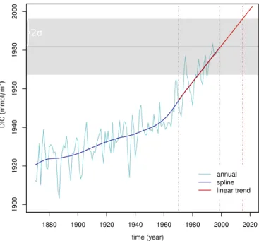
whereSis the trend andNa measure for variability. For each grid cell,Sis defined as the linear trend (per year) over the period 1970–1999. A different approach is the com-putation of the trend by applying a smoothing spline on the time series; test calculations for 1970–1999 yield comparable results. Figure 1 exemplarily illustrates the two approaches and the good agreement between them based on the model NCAR CESM1. We note that by also applying the linear trend from the 1970 to 1999 period in the future, any changes in trends are not explicitly accounted for. Changes in trends are likely to remain relatively small in the next few decades, but trends will differ considerably between business-as-usual and stringent mitigation scenarios by the end of this cen-tury (e.g., Steinacher et al., 2009; Cocco et al., 2013; Bopp et al., 2013). ForN, the standard deviation (SD) over the en-tire simulation, 1870–1999, is used. Prior to this last step, the data are detrended via a spline approach (cut-off period: 40 yr; Enting, 1987).
For illustration purposes, we calculate ToE for DIC at a lo-cation in the subtropical North Pacific (see also Fig. 1). By in-serting the respective values forS(0.94 mmol m−3yr−1) and
N (7.24 mmol m−3), we obtain (2×7.24)/0.94=15.4 yr,
that is, a (rounded up) ToE of 16 yrs. The ensemble mean of ToE is computed from the ToE of individual models, and not from the ensemble mean ofSandN. Note that the pre-sented ensemble mean patterns, i.e., the averages of all 17 models, are not necessarily physically consistent.
time (year)
DIC
(
mmol
m
3)
1880 1900 1920 1940 1960 1980 2000 2020
annual spline linear trend
}
2σ1900
1920
1940
1960
1980
2000
Figure 1. NCAR CESM1: annual time series (light blue), corre-sponding smoothing spline (dark blue), and linear trend (red) of dissolved inorganic carbon (DIC; mmol m−3) at 22◦N, 158◦W, the proximate location of the Hawaii Ocean Time-series (HOT; Keeling et al., 2004). The grey bar represents two times the standard devia-tion of the detrended time series (i.e., annual-spline). The spline is calculated with a cut-off period of 40 yr. The linear trend is based on the years 1970–1999 of annual, as indicated by the grey verti-cal lines. The intersect between the red vertiverti-cal line and the upper border of the grey bar (x=2015) shows when the trend leaves the envelope of background variability and, from then on, is detectable. Consequently, the ToE at this location is 16 yr (2015–1999).
Ilyina and Zeebe, 2012) or the range of the pre-industrial an-nual cycle (Friedrich et al., 2012). Here, we use the rather conservative value of two SDs of interannual variability. For a threshold of one SD, the ToE would be half, accordingly.
By calculatingS over a time period of 30 yr, to a certain degree we can rule out interference of low-frequency vari-ability in the detection of the trend (see e.g., McKinley et al., 2011). A ToE of only a few decades, as is especially the case for the three carbon cycle variables (see Sect. 3.1), is thus a strong indicator for the significance of the respective trend. This is confirmed by a significance test (t test, 5 % level) of the trend of the underlying 30 yr time series (not shown): for all 17 models, all trends in pH are significant. The trends inpCO2are also significant, yet with localized
in-significant exceptions in the Southern Ocean (BCCR BCM-C, IPSL-CM5A-MR) and the upwelling region off Peru and Chile (CanESM2). Trends in DIC are significant in large parts of the global oceans, exceptions are the high latitudes and the equatorial Pacific. Statistically significant trends in SST are less widespread and corresponding regional results are highly model-dependent.
In using these definitions, we assume that (i) the trend from 1970 to 1999 is linear, (ii) the SD is constant over time and, by using annual averages, (iii) that trends and SD pat-terns are comparable for annual, seasonal or monthly data. To verify (i), the global trends of surface DIC and SST for the period 1970–1999 are investigated. For all models, we find that trends in global surface DIC can be represented by a linear function. SST shows larger inter-annual variability, yet likewise with a linear underlying trend. For (ii), we in-vestigate the detrended data (1870–1999) of DIC and SST of all 17 models (not shown). The comparison of SD fields cal-culated for the first and second 65 yr (F test, 5 % level) illus-trates that differences only occur in very localized instances, consequently we suggest that this assumption is confirmed. Assumption (iii) can be confirmed for the trend patterns. The standard deviations, however, differ considerably in magni-tude – we address this issue in Sect. 3.2.
3 Results and discussion
In the ocean, observations are scarce and often limited in time, e.g., to specific seasons. We address this by splitting our analysis in two parts. First, the complete model ensem-ble is used to investigate the “best case” with respect to ob-servations, i.e., complete annual data coverage (Sect. 3.1). In a second step, and based on two individual models, the focus is on the months January and July to estimate the impact of seasonality (Sect. 3.2).
3.1 ToE – ensemble mean
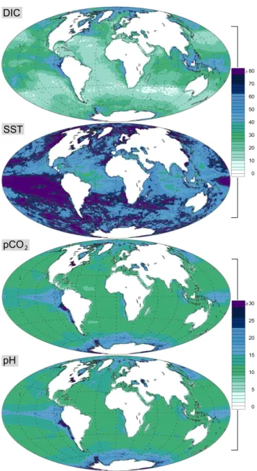
Figure 2 shows the ensemble mean ToE patterns of dissolved inorganic carbon (DIC),pCO2, pH and sea-surface
tempera-ture (SST), all variables on surface level. We find that trend signals in the three carbon cycle variables emerge on much shorter timescales than the physical climate variable SST. The ToE pattern of SST is very noisy, varying typically be-tween 45 and 90 yr. The exception are areas around the equa-tor in the Atlantic, Indian and western Pacific Ocean, with values of approximately 35 yr. A large coherent area with ToE>80 yr can be found in the (eastern) equatorial Pacific. The trend in DIC appears in large parts of the global oceans after approximately 10–30 yr; higher values are found at high latitudes, especially the Arctic Ocean (≈50 yr), and local-ized in the equatorial Pacific (up to≈70 yr). ToE ofpCO2
and pH show a very similar pattern. However, the trends emerge much faster for pCO2 and pH than for DIC: after
≈12 yr for the majority of the global ocean area, 14–18 yr in the Arctic Ocean and ≈20 yr in the equatorial Pacific. A likely reason for these different timescales of DIC and pH/pCO2 are nonlinear processes in ocean chemistry
de-scribed by the buffer factor (or Revelle factor; Revelle and Suess, 1957), which result in increases ofpCO2of
DIC
SST
pCO2
pH
≥80 70
60
50
40
30
20
10
0
≥30
25
20
15
10
5
0
Figure 2. ToE (years) of dissolved inorganic carbon (DIC; mmol m−3), sea-surface temperature (SST;◦C),pCO2(ppmv), and
total pH. Ensemble mean, all variables on surface level. Note the different scales for DIC/SST andpCO2/pH.
increases in DIC. In contrast to DIC, relatively high ToE val-ues are found for bothpCO2and pH in the Southern Ocean
and in the upwelling region off Peru and Chile (both regions, localized>30 yr). Taking past changes since the beginning of the industrialization into account, the low ToE values, es-pecially forpCO2and pH, indicate that anthropogenic trends
are already detectable in large parts of the global surface oceans. This is in agreement with Mora et al. (2013) for pH and Friedrich et al. (2012) concerning the saturation state of aragonite (A), another measure for ocean acidification.
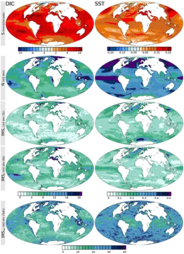
A direct evaluation of ToE is difficult, if not impossible, due to the lack of suitable observations. However, it is fea-sible for the underlying fields signalSand noiseN (Fig. 3a and 3b). These two variables are of added value since they allow determining the importance of S and N for the re-sulting ToE fields. The top row of Fig. 3a and 3b shows S, the trend/decade over the years 1970–1999, the second row illustratesN, the standard deviation of the (detrended) years 1870–1999. To evaluate these patterns, we compiled a number of observations (Table 1). These time series re-markably illustrate the importance of natural variability. The Bermuda Time Series Station (BATS), located near Bermuda in the North Atlantic, and Station ALOHA, the site of the US JGOFS Hawaii Ocean Time-series program (HOT) located in the central North Pacific, contribute trends over multiple yet overlapping time periods. It is striking how a different start (BATS) or end (ALOHA) year can change the trend es-timation of a time series. At ALOHA, trends of DIC and SST even switch from negative to positive and vice versa, depending on the time period. This issue is addressed in a re-cent study by Fay and McKinley (2013). These authors in-vestigated trends in surface oceanpCO2 measurements
be-tween 1981 and 2010 for periods of 4 yr to up to 30 yr. They found that, on shorter timescales, trends of surfacepCO2are
sensitive to variability presumably linked to climatic oscil-lations and, consequently, may vary between different peri-ods. Accordingly, this caveat has to be taken into account when comparing modeled and observed trends over relatively short time periods. Fay and McKinley also find that the in-fluence of climatic oscillations fades when analysis periods are between 25 and 30 yr, as used in this study to determine trends. We note that a direct comparison between the trend signals computed by Fay and McKinley and our trend sig-nal is hampered by the fact that Fay and McKinley use rela-tively sparse observational data to determine trends. Conse-quently, a comparison of modeled and observed trends has to be undertaken with caution. For DIC, features like a stronger trend at BATS compared to ESTOC are captured by the en-semble mean. Overall, however, the models slightly under-estimate the observed trends by up to 5 mmol m−3yr−1. For
pCO2, both model mean and observations show robust
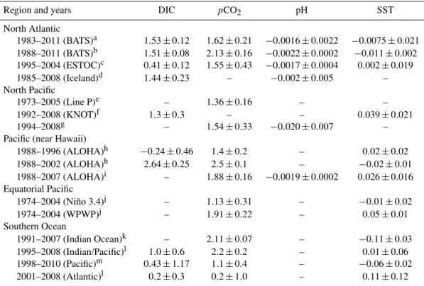
Table 1.Observed trends/year of dissolved inorganic carbon (DIC; mmol m−3),pCO2(ppmv or µatm), total pH and sea-surface temperature
(SST;◦C), all variables on surface level. Note that we include only directly measured DIC, that is, not salinity-normalized.
Region and years DIC pCO2 pH SST
North Atlantic
1983–2011 (BATS)a 1.53±0.12 1.62±0.21 −0.0016±0.0022 −0.0075±0.021 1988–2011 (BATS)b 1.51±0.08 2.13±0.16 −0.0022±0.0002 −0.011±0.002 1995–2004 (ESTOC)c 0.41±0.12 1.55±0.43 −0.0017±0.0004 0.002±0.019 1985–2008 (Iceland)d 1.44±0.23 – −0.002±0.005 – North Pacific
1973–2005 (Line P)e – 1.36±0.16 – – 1992–2008 (KNOT)f 1.3±0.3 – – 0.039±0.021 1994–2008g – 1.54±0.33 −0.020±0.007 – Pacific (near Hawaii)
1988–1996 (ALOHA)h −0.24±0.46 1.4±0.2 – 0.02±0.02 1988–2002 (ALOHA)h 2.64±0.25 2.5±0.1 – −0.02±0.01 1988–2007 (ALOHA)i – 1.88±0.16 −0.0019±0.0002 0.026±0.016 Equatorial Pacific
1974–2004 (Niño 3.4)j – 1.13±0.31 – −0.01±0.02 1974–2004 (WPWP)j – 1.91±0.22 – 0.05±0.01 Southern Ocean
1991–2007 (Indian Ocean)k – 2.11±0.07 – −0.11±0.03 1995–2008 (Indian/Pacific)l 1.0±0.6 2.2±0.2 – 0.01±0.06 1998–2010 (Pacific)m 0.43±1.17 1.1±0.4 – −0.06±0.02 2001–2008 (Atlantic)l 0.2±0.3 0.2±1.0 – 0.11±0.12
aBates et al. (2012),bBates (2012),cSantana-Casiano et al. (2007),dOlafsson et al. (2009),eWong et al. (2010),fWakita et al. (2010),g
Ishii et al. (2011),hKeeling et al. (2004),iDore et al. (2009),jFeely et al. (2006),kMetzl (2009),lLenton et al. (2013),
mBrix et al. (2013).
on annual means, we calculate trend and standard deviation over the period 1970–1999 (not shown). The ensemble mean trend pattern captures the main features of the reanalysis, with comparably strong trends in the equatorial and North Pacific, and the North Atlantic. However, the modeled trends are slightly lower and in general more homogeneous. The reanalysis shows a stronger gradient between regions with strong and very weak trends. Further, the reanalysis shows negative trends in the Pacific from 20 to 40◦N, which are not present in the ensemble mean. Globally, we find a pattern correlationrbetween model ensemble and reanalysis of 0.44 (90–20◦S: 0.56; 20◦S–20◦N: 0.36; and 20–90◦N: 0.68). Concerning standard deviation, the picture is similar. Both ensemble mean and reanalysis capture main variability fea-tures such as the ENSO region or parts of the North Atlantic. However, again the ensemble mean is more homogeneous. The reanalysis indicates very low inter-annual variability in the high latitudes, especially the Southern Ocean, which is not the case for the model ensemble. We find a global pattern correlationrof 0.88 (90–20◦S: 0.82; 20◦S–20◦N: 0.81; and 20–90◦N: 0.89).
To evaluate N, we can verify the presence of main char-acteristics of natural variability. One prominent feature is El Niño–Southern Oscillation (ENSO; Fiedler, 2002), located in the equatorial Pacific. This climate mode, the most
impor-tant factor concerning natural variability in the climate sys-tem on global scales, is known to have substantial impact on the ocean carbon cycle in the affected area (e.g., Le Quéré et al., 2010; Wanninkhof et al., 2013) and the global air–sea CO2 flux in general (Siegenthaler, 1990; McKinley et al.,
2004). We find clear indications of ENSO in the SD pat-terns of SST, DIC andpCO2, and a weak signal for pH.
An-other area of high natural variability is the North Atlantic, which is influenced by modes like the North Atlantic Oscil-lation (NAO; Hurrell and Deser, 2009) or changes in the At-lantic Meridional Overturning Circulation (AMOC; Carton and Häkkinen, 2011), both known for affecting the ocean car-bon cycle (e.g., Keller et al., 2012; Perez et al., 2013). A fur-ther region with high variability in the ocean carbon system is the Southern Ocean (see e.g., Bacastow, 1976; Marinov et al., 2006; Lovenduski et al., 2007; Le Quéré et al., 2007; Resplandy et al., 2013b), where we find a corresponding sig-nal in the ensemble SDpCO2pattern.
Figure 3a.Trend per decade (S), standard deviation (N) and, as measures for the inter-model spread (IMS), standard deviations of
S(IMSS),N(IMSN), and ToE (IMSToE; years) of dissolved
inor-ganic carbon (DIC; mmol m−3) and sea-surface temperature (SST;
◦C).
alone, asS shows medium levels. The opposite is the case in the North Pacific, where high ToE is caused by weak trend signals. The ToE pattern ofpCO2seems to be dominated by
N, supported by anti-correlated lowSon local scales in the Southern Ocean. N of pH is relatively homogeneous, with elevated variability levels in the Arctic Ocean, the Southern Ocean and, locally, the eastern equatorial Pacific. These ar-eas imprint on the ToE pattern, yetSseems to be more im-portant. For the carbon cycle variables,SandNare found to be anti-correlated in some regions. The opposite is the case for SST, which shows both high trends and variability in the equatorial Pacific, the North Pacific, and parts of the North Atlantic. The associated high ToE values illustrate the dom-inance ofN, which masks the strong trends in these areas. In the equatorial parts of the Atlantic, western Pacific and Indian Ocean, the absence of strong variability allowsS to govern the ToE field. In conclusion, we see that in areas with high natural variability, even strong trends both in the
physi-Figure 3b.Trend per decade (S), standard deviation (N) and, as measures for the inter-model spread (IMS), standard deviations of
S(IMSS),N(IMSN), and ToE (IMSToE; years) ofpCO2(ppmv)
and total pH.
cal climate and carbon cycle system are masked over decadal timescales.
When working with a model ensemble, it is important to consider the inter-model spread (IMS). It illustrates where and when the models diverge and is thus a measure for uncer-tainty. Figure 3a and 3b show the standard deviation across all 17 models ofS (IMSS),N (IMSN) and ToE (IMSToE).
The four IMSS fields show related patterns, with high IMS
in the Southern Ocean (all four variables), the Arctic Ocean (DIC and, weaker, pH and pCO2) and the North Atlantic
(SST). The IMSNfield of SST mirrors the pattern of IMSSin
the North Atlantic, and the same is true for DIC in the sub-tropical Pacific and the eastern Arctic Ocean. IMSN of pH
indicates a large-scale zonal structure and shows, together withpCO2, high IMS in the upwelling region off Peru and
Chile. The IMSToE field of DIC resembles the pattern for
N, with high IMS in the Arctic and the equatorial Pacific Ocean. IMSToEof pH andpCO2are much alike, with large
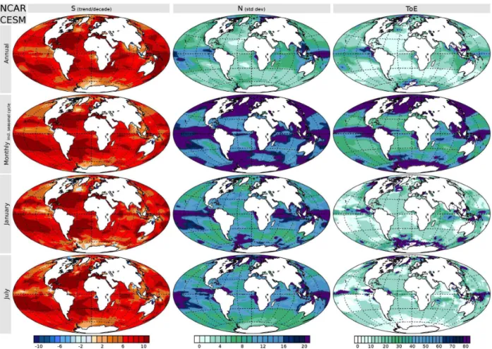
Figure 4.NCAR CESM1: Trend per decade (S), standard deviation (N) and ToE (years) of dissolved inorganic carbon (DIC; mmol m−3)
for the period 1975–2004.SandNare calculated on a basis of annual averages (#30, row 1), monthly averages, including full seasonal cycle (#360, row 2), January only (#30, row 3), and July only (#30, row 4).
with generally lower values around the equator. Possible rea-sons for the model spread in the Southern Ocean include the inadequate representation of bottom-water formation pro-cesses in many CMIP5 models (Heuzé et al., 2013) and a sys-tematic wind bias inherent to many models, which impacts physical processes like Antarctic Circumpolar Current and Southern Ocean water mass formation and, consequently, the ocean carbon cycle (Swart and Fyfe, 2012). In areas with high natural variability, such as the equatorial Pacific or the North Atlantic, IMS might arise from differences in time and space of the representation of climate modes such as ENSO or NAO (e.g., Keller et al., 2012). Another possible factor is the model resolution, especially in areas dominated by local processes such as coastal upwelling.
3.2 Impact of seasonality
For 6 out of 17 models, we have monthly data available. These are NCAR CESM1 (the complete simulation, 1850– 2005), NCAR CCSM3-BEC and NCAR CSM1.4-carbon (25 yr, 1985–2009), and BCCR BCM-C, IPSL-CM4 and COSMOS (30 yr, 1980–2009). A comparison based on an-nual averages of the complete 130 yr and the monthly data
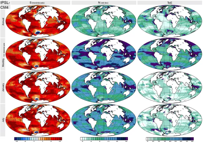
(NCAR CESM1: 1975–2004) provides very similar results. Accordingly, we assume that time periods of 25 and 30 yr are sufficient to capture main variability features and that results based on this data are robust. As mentioned in Sect. 2, we find that the trend patterns of all four variables are indeed comparable for the different timescales. The fields of stan-dard deviation, however, differ. The regions mainly affected by intra-annual variability are the high latitudes. For DIC, as an example, the monthly averages over the time series dis-play a clear seasonal cycle for four out of six models (NCAR CESM1, CCSM3-BEC, NCAR CSM1.4-carbon and COS-MOS), while others show comparably homogeneous patterns throughout the year (BCCR BCM-C, IPSL-CM4). For both pH andpCO2we find seasonal signals for the models NCAR
Figure 5.IPSL-CM4: Trend per decade (S), standard deviation (N) and ToE (years) of dissolved inorganic carbon (DIC; mmol m−3) for the period 1980–2009.SandNare calculated on a basis of annual averages (#30, row 1), monthly averages, including full seasonal cycle (#360, row 2), January only (#30, row 3), and July only (#30, row 4).
Figures 4 and 5 show S, N and ToE of surface DIC for the models NCAR CESM1 and IPSL-CM4, respectively. The fields are calculated using the same 30 yr of monthly data (NCAR: 1975–2004, IPSL: 1980–2009), albeit with different temporal resolutions: annual averages (#30, row 1), monthly averages, including full seasonal cycle (#360, row 2), Jan-uary only (#30, row 3) and July only (#30, row 4). For case two (monthly averages), an alternative approach would be to define N as the full range of the seasonal cycle. In do-ing so, it is possible to make a clear distinction between inter- and intra-annual variability. However, we focus on the combination of both since it is closer to what we find in re-ality. For both models,S is comparable concerning magni-tude and spatial patterns in all four cases. One exception is the area around (IPSL) or east of Australia (CESM), which shows strong trends in the annual averages. A comparison of the cases “Annual” and “Monthly” illustrates the expected loss of variability due to temporal averaging, especially in this case where the seasonal cycle is still present in the monthly data. Consistent with the ensemble mean, the two “Annual”N fields show variability hot-spots in the equato-rial Pacific and, locally, the Arctic Ocean. When the seasonal
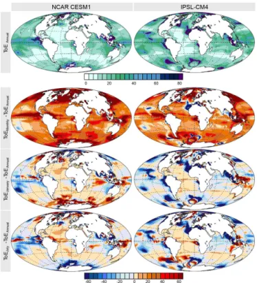
Figure 6.NCAR CESM1 and IPSL-CM4: ToE “Annual” (row 1; same as in Figs. 4 and 5) and, for the cases “Monthly” (row 2), “January” (row 3), and “July” (row 4), the offset relative to this case (e.g., row 2: ToEMonthly–ToEAnnual).
2), “January” (row 3) and “July” (row 4), the offset relative to this case (e.g., row 2: ToEMonthly–ToEAnnual). ToE “Monthly”
of both models shows the expected substantially later ToE as the “Annual” case. “January” and “July” show compara-ble (±10 yr) ToE to the “Annual” case in large parts of the global oceans, especially in the low and middle latitudes. However, the NCAR model shows large deviations (up to ±60 yr and more) in the high latitudes, the equatorial Pa-cific, the Indian Ocean and, more localized, in other areas. This has important implications for observations. The “Jan-uary/July” patterns are similar in parts of the global oceans. This indicates that, at these locations, statements based on ir-regularly sampled data are valid representatives for the whole year. In large areas, however, intra-annual variability might interfere such a generalization. An illustrative example is the slowdown of the AMOC, which was suggested by Bryden et al. (2005) based on five cross sections in the North At-lantic. These snap-shot measurements were distributed over the seasons in such a way that they embraced the full range of the seasonal cycle, and the observed slow-down was later at-tributed mainly to “aliasing due to seasonal anomalies” (Kan-zow et al., 2010).
4 Conclusions
Here, we investigate the time of emergence (ToE) of trends in the surface ocean carbon cycle utilizing an ensemble of 17 state-of-the-art ESMs. The ToE is the time required until a sustained trend exceeds a variability threshold (here two standard deviations). Thus, ToE depends on reliable esti-mates of both trend and variability. For example, an under-estimation of the variability in the model compared to the real ocean would bias ToE towards low values. Yet, the study shows that the ensemble mean trend and standard deviation patterns are in reasonable agreement with observations and reanalysis data sets, which supports the robustness of the pre-sented results.
ToE of pH andpCO2has rather low values (around 10 yr)
in many regions of the surface ocean. It is, however, gener-ally difficult if not impossible to reliably determine variabil-ity and long-term trends in the surface ocean from data that extend over such a short period only. Trends in surface ocean variables can vary significantly between different 10 yr peri-ods and even reverse sign (see Fig. 1 and Table 1, ALOHA data for an illustration). As a consequence, model data, or measurements, over a longer period are needed to reliably determine anthropogenic trends (Fay and McKinley, 2013) and the ToE. Here, trends and variability are estimated from 30 yr (1970 to 1999) and 130 yr of model data, respectively. The choice of a 30 yr period minimizes the influence of cli-mate modes such as NAO, ENSO or AMOC on trends as demonstrated by Fay and McKinley (2013) for surface ocean pCO2 measurements, while at the same time the 1970 to
2000 period still provides an approximate measure of the cur-rent and near-future anthropogenic trend in the surface ocean. The ToE is indicative for the time required for the anthro-pogenic trend to leave the variability band, but it should not be confused with the period required to detect this trend in observational or model data.
We find that trend signals in ocean biogeochemical vari-ables emerge on much shorter timescales than the physical climate variable SST. ToE fields ofpCO2and pH are
spa-tially very similar to DIC, yet emerge much faster – after ≈12 yr for the majority of the global ocean area, compared to≈10–30 yr for DIC. Assuming that natural variability is constant over time, we suggest that possible stronger future trends would emerge accordingly faster. We find that, in gen-eral, the standard deviation is of higher importance in deter-mining ToE than the strength of the linear trend. In areas with high natural variability, even strong trends both in the physi-cal climate and carbon cycle system are masked by variabil-ity over decadal timescales. This explains inconsistencies in trends based on time series of insufficient length to overcome natural variability, and illustrates the necessity for long-term observations.
already detectable in large parts of the global oceans. This finding is even more relevant as the highest rates of ocean acidification are measured (Bates, 2012; Dore et al., 2009) and modeled (Resplandy et al., 2013a) in subsurface waters. A further finding of the study is that, in contrast to the trend, the standard deviation is affected by the seasonal cycle. This has important implications for the use of sparse observa-tions. In some parts of the global oceans, there are hints that statements based on irregularly sampled seasonal data might be representative for the whole year. In large areas, however, intra-annual variability might interfere such a generalization. The study clearly illustrates the need for more long-term measurements with sufficient seasonal data coverage. DIC is a very important variable and crucial for our understand-ing of processes. For the sole detection of trends, however, pCO2and pH seem to be a better choice. Further,
observa-tions are not only necessary for the correct detection of trends and natural variability. Independent data sets are also key for the robust forcing and evaluation of climate models which are, since observations are still scarce, the measure of choice for many research questions.
Acknowledgements. We thank Juliette Mignot and Jim Orr for discussion and comments. The research leading to these results was supported through EU FP7 project CARBOCHANGE “Changes in carbon uptake and emissions by oceans in a changing climate”, which received funding from the European Community’s Seventh Framework Programme under grant agreement no. 264879. Additional support was received from the Swiss National Science Foundation. We thank IPSL and ETHZ for providing the model data of OCMIP5 and CMIP5. Simulations with NCAR CESM1 were carried out at the Swiss National Supercomputing Centre in Lugano, Switzerland.
Edited by: L. Cotrim da Cunha
References
Assmann, K. M., Bentsen, M., Segschneider, J., and Heinze, C.: An isopycnic ocean carbon cycle model, Geosci. Model Dev., 3, 143–167, doi:10.5194/gmd-3-143-2010, 2010.
Aumont, O., Maier-Reimer, E., Blain, S., and Monfray, P.: An ecosystem model of the global ocean including Fe, Si, P colimitations, Global Biogeochem. Cy., 17, 1060, doi:10.1029/2001GB001745, 2003.
Bacastow, R. B.: Modulation of atmospheric carbon dioxide by the Southern Oscillation, Nature, 261, 116–118, 1976.
Bates, N. R.: Multi-decadal uptake of carbon dioxide into subtropi-cal mode water of the North Atlantic Ocean, Biogeosciences, 9, 2649–2659, doi:10.5194/bg-9-2649-2012, 2012.
Bates, N. R., Best, M. H. P., Neely, K., Garley, R., Dickson, A. G., and Johnson, R. J.: Detecting anthropogenic carbon dioxide up-take and ocean acidification in the North Atlantic Ocean, Bio-geosciences, 9, 2509–2522, doi:10.5194/bg-9-2509-2012, 2012. Bopp, L., Resplandy, L., Orr, J. C., Doney, S. C., Dunne, J. P., Gehlen, M., Halloran, P., Heinze, C., Ilyina, T., Séférian, R.,
Tjiputra, J., and Vichi, M.: Multiple stressors of ocean ecosys-tems in the 21st century: projections with CMIP5 models, Biogeosciences, 10, 6225–6245, doi:10.5194/bg-10-6225-2013, 2013.
Brix, H., Currie, K. I., and Mikaloff Fletcher, S. E.: Seasonal vari-ability of the carbon cycle in subantarctic surface water in the South West Pacific, Global Biogeochem. Cy., 27, 200–211, 2013. Bryden, H. L., Longworth, H. R., and Cunningham, S. A.: Slow-ing of the Atlantic meridional overturnSlow-ing circulation at 25◦N, Nature, 438, 655–657, 2005.
Carton, J. A. and Häkkinen, S.: Introduction to: Atlantic Merid-ional Overturning Circulation (AMOC), Deep-Sea Res. Pt. II, 58, 1741–1743, 2011.
Christian, J. R., Arora, V. K., Boer, G. J., Curry, C. L., Zahariev, K., Denman, K. L., Flato, G. M., Lee, W. G., Merryfield, W. J., Roulet, N. T., and Scinocca, J. F.: The global carbon cycle in the Canadian Earth system model (CanESM1): preindus-trial control simulation, J. Geophys. Res.-Biogeo., 115, G03014, doi:10.1029/2008JG000920, 2010.
Cocco, V., Joos, F., Steinacher, M., Frölicher, T. L., Bopp, L., Dunne, J., Gehlen, M., Heinze, C., Orr, J., Oschlies, A., Schnei-der, B., SegschneiSchnei-der, J., and Tjiputra, J.: Oxygen and indicators of stress for marine life in multi-model global warming projec-tions, Biogeosciences, 10, 1849–1868, doi:10.5194/bg-10-1849-2013, 2013.
Collins, W. D., Bitz, C. M., Blackmon, M. L., Bonan, G. B., Bretherton, C. S., Carton, J. A., Chang, P., Doney, S. C., Hack, J. J., Henderson, T. B., Kiehl, J. T., Large, W. G., McKenna, D. S., Santer, B. D., and Smith, R. D.: The Commu-nity Climate System Model version 3 (CCSM3), J. Climate, 19, 2122–2143, 2006.
Diffenbaugh, N. and Giorgi, F.: Climate change hotspots in the CMIP5 global climate model ensemble, Climatic Change, 114, 813–822, 2012.
Diffenbaugh, N. and Scherer, M.: Observational and model evi-dence of global emergence of permanent, unprecedented heat in the 20th and 21st centuries, Climatic Change, 107, 615–624, 2011.
Dolman, A. J., van der Werf, G. R., van der Molen, M. K., Ganssen, G., Erisman, J. W., and Strengers, B.: A carbon cycle science update since IPCC AR-4, Ambio, 39, 402–412, 2010. Doney, S. C., Lindsay, K., Fung, I., and John, J.: Natural variability
in a stable, 1000-yr global coupled climate-carbon cycle simula-tion, J. Climate, 19, 3033–3054, 2006.
Dore, J. E., Lukas, R., Sadler, D. W., Church, M. J., and Karl, D. M.: Physical and biogeochemical modulation of ocean acidification in the central North Pacific, P. Natl. Acad. Sci. USA, 106, 12235– 12240, 2009.
Dunne, J. P., John, J. G., Shevliakova, E., Stouffer, R. J., Krast-ing, J. P., Malyshev, S. L., Milly, P. C. D., Sentman, L. T., Ad-croft, A. J., Cooke, W., Dunne, K. A., Griffies, S. M., Hall-berg, R. W., Harrison, M. J., Levy, H., WittenHall-berg, A. T., Phillips, P. J., and Zadeh, N.: GFDL’s ESM2 Global coupled climate–carbon Earth System Models. Part II: Carbon system formulation and baseline simulation characteristics, J. Climate, 26, 2247–2267, 2012.
Enting, I. G.: On the use of smoothing splines to filter CO2data, J.
Geophys. Res.-Atmos., 92, 10977–10984, 1987.
Fay, A. R. and McKinley, G. A.: Global trends in surface ocean
pCO2from in situ data, Global Biogeochem. Cy., 27, 541–557,
2013.
Feely, R. A., Takahashi, T., Wanninkhof, R., McPhaden, M. J., Cosca, C. E., Sutherland, S. C., and Carr, M.-E.: Decadal variability of the air-sea CO2 fluxes in the equatorial
Pacific Ocean, J. Geophys. Res.-Oceans, 111, C08S90, doi:10.1029/2005JC003129, 2006.
Fiedler, P.: Environmental change in the eastern tropical Pacific Ocean: review of ENSO and decadal variability, Mar. Ecol.-Prog. Ser., 244, 265–283, 2002.
Friedrich, T., Timmermann, A., Abe-Ouchi, A., Bates, N. R., Chikamoto, M. O., Church, M. J., Dore, J. E., Gled-hill, D. K., Gonzalez-Davila, M., Heinemann, M., Ilyina, T., Jungclaus, J. H., McLeod, E., Mouchet, A., and Santana-Casiano, J. M.: Detecting regional anthropogenic trends in ocean acidification against natural variability, Nat. Clim. Change, 2, 167–171, 2012.
Frölicher, T. L., Joos, F., Plattner, G. K., Steinacher, M., and Doney, S. C.: Natural variability and anthropogenic trends in oceanic oxygen in a coupled carbon cycle-climate model ensemble, Global Biogeochem. Cy., 23, GB1003, doi:10.1029/2008GB003316, 2009.
Giorgi, F. and Bi, X.: Time of emergence (TOE) of GHG-forced precipitation change hot-spots, Geophys. Res. Lett., 36, L06709, doi:10.1029/2009GL037593, 2009.
Hauri, C., Gruber, N., Vogt, M., Doney, S. C., Feely, R. A., Lachkar, Z., Leinweber, A., McDonnell, A. M. P., Munnich, M., and Plattner, G.-K.: Spatiotemporal variability and long-term trends of ocean acidification in the California Current Sys-tem, Biogeosciences, 10, 193–216, doi:10.5194/bg-10-193-2013, 2013.
Hawkins, E. and Sutton, R.: Time of emergence of climate signals, Geophys. Res. Lett., 39, L01702, doi:10.1029/2011GL050087, 2012.
Hegerl, G. C., Zwiers, F. W., Braconnot, P., Gillett, N., Luo, Y., Orsini, J. M., Nicholls, N., Penner, J., and Stott, P.: Understand-ing and attributUnderstand-ing climate change, in: Climate Change 2007: The Physical Science Basis, Contribution of Working Group I to the Fourth Assessment Report of the Intergovernmental Panel on Climate Change, edited by: Solomon, S., Qin, D., Man-ning, M., Chen, Z., Marquis, M., Averyt, K. B., Tignor, M., and Miller, H. L., Cambridge University Press, Cambridge, UK and New York, NY, USA, 2007.
Heuzé, C., Heywood, K. J., Stevens, D. P., and Ridley, J. K.: South-ern Ocean bottom water characteristics in CMIP5 models, Geo-phys. Res. Lett., 40, 1409–1414, 2013.
Hurrell, J. W. and Deser, C.: North Atlantic climate variability: the role of the North Atlantic Oscillation, J. Mar. Syst., 78, 28–41, 2009.
Ilyina, T. and Zeebe, R. E.: Detection and projection of carbon-ate dissolution in the wcarbon-ater column and deep-sea sediments due to ocean acidification, Geophys. Res. Lett., 39, L06606, doi:10.1029/2012GL051272, 2012.
Ilyina, T., Zeebe, R. E., Maier-Reimer, E., and Heinze, C.: Early detection of ocean acidification effects on
ma-rine calcification, Global Biogeochem. Cy., 23, GB1008, doi:10.1029/2008GB003278, 2009.
Ilyina, T., Six, K. D., Segschneider, J., Maier-Reimer, E., Li, H., and Núñez-Riboni, I.: Global ocean biogeochemistry model HAMOCC: model architecture and performance as component of the MPI-Earth system model in different CMIP5 experi-mental realizations, J. Adv. Model. Earth Syst., 5, 287–315, doi:10.1029/2012MS000178, 2013.
Ishii, M., Kosugi, N., Sasano, D., Saito, S., Midorikawa, T., and Inoue, H. Y.: Ocean acidification off the south coast of Japan: a result from time series observations of CO2
parame-ters from 1994 to 2008, J. Geophys. Res.-Oceans, 116, C06022, doi:10.1029/2010JC006831, 2011.
Joos, F., Plattner, G., Stocker, T., Marchal, O., and Schmittner, A.: Global warming and marine carbon cycle feedbacks on future atmospheric CO2, Science, 284, 464–467, 1999.
Jungclaus, J. H., Keenlyside, N., Botzet, M., Haak, H., Luo, J. J., Latif, M., Marotzke, J., Mikolajewicz, U., and Roeckner, E.: Ocean circulation and tropical variability in the coupled model ECHAM5/MPI-OM, J. Climate, 19, 3952–3972, 2006.
Kanzow, T., Cunningham, S. A., Johns, W. E., Hirschi, J. J.-M., Marotzke, J., Baringer, M. O., Meinen, C. S., Chidichimo, M. P., Atkinson, C., Beal, L. M., Bryden, H. L., and Collins, J.: Sea-sonal variability of the Atlantic Meridional Overturning Circula-tion at 26.5◦N, J. Climate, 23, 5678–5698, 2010.
Karoly, D. J. and Wu, Q.: Detection of regional surface temperature trends, J. Climate, 18, 4337–4343, 2005.
Keeling, C. D., Brix, H., and Gruber, N.: Seasonal and long-term dynamics of the upper ocean carbon cycle at Station ALOHA near Hawaii, Global Biogeochem. Cy., 18, GB4006, doi:10.1029/2004GB002227, 2004.
Keeling, R. F., Körtzinger, A., and Gruber, N.: Ocean deoxygena-tion in a warming world, Annu. Rev. Mar. Sci., 2, 199–229, 2010. Keller, K., Joos, F., Raible, C., Cocco, V., Frölicher, T., Dunne, J., Gehlen, M., Bopp, L., Orr, J., Tjiputra, J., Heinze, C., Segschnei-der, J., Roy, T., and Metzl, N.: Variability of the ocean carbon cycle in response to the North Atlantic Oscillation, Tellus B, 64, 18738, doi:10.3402/tellusb.v64i0.18738, 2012.
Latif, M., Kleeman, R., and Eckert, C.: Greenhouse warming, decadal variability, or El Niño? An attempt to understand the anomalous 1990s, J. Climate, 10, 2221–2239, 1997.
Le Quéré, C., Roedenbeck, C., Buitenhuis, E. T., Conway, T. J., Langenfelds, R., Gomez, A., Labuschagne, C., Ramonet, M., Nakazawa, T., Metzl, N., Gillett, N., and Heimann, M.: Satu-ration of the Southern Ocean CO2sink due to recent climate
change, Science, 316, 1735–1738, 2007.
Le Quéré, C., Takahashi, T., Buitenhuis, E. T., Roedenbeck, C., and Sutherland, S. C.: Impact of climate change and variability on the global oceanic sink of CO2, Global Biogeochem. Cy., 24,
GB4007, doi:10.1029/2009GB003599, 2010.
Lenton, A., Tilbrook, B., Law, R. M., Bakker, D., Doney, S. C., Gru-ber, N., Ishii, M., Hoppema, M., Lovenduski, N. S., Matear, R. J., McNeil, B. I., Metzl, N., Mikaloff Fletcher, S. E., Mon-teiro, P. M. S., Rödenbeck, C., Sweeney, C., and Takahashi, T.: Sea–air CO2fluxes in the Southern Ocean for the period 1990– 2009, Biogeosciences, 10, 4037–4054, doi:10.5194/bg-10-4037-2013, 2013.
sea-level commitment of global warming, P. Natl. Acad. Sci. USA, 110, 13745–13750, 2013.
Lovenduski, N. S., Gruber, N., Doney, S. C., and Lima, I. D.: En-hanced CO2outgassing in the Southern Ocean from a positive
phase of the Southern Annular Mode, Global Biogeochem. Cy., 21, GB2026, doi:10.1029/2006GB002900, 2007.
Mahlstein, I., Knutti, R., Solomon, S., and Portmann, R. W.: Early onset of significant local warming in low latitude countries, Env-iron. Res. Lett., 6, 034009, doi:10.1088/1748-9326/6/3/034009, 2011.
Mahlstein, I., Hegerl, G., and Solomon, S.: Emerging local warming signals in observational data, Geophys. Res. Lett., 39, L21711, doi:10.1029/2012GL053952, 2012.
Mahlstein, I., Daniel, J. S., and Solomon, S.: Pace of shifts in climate regions increases with global temperature, Nat. Clim. Change, 3, 739–743, 2013.
Marinov, I., Gnanadesikan, A., Toggweiler, J., and Sarmiento, J.: The Southern Ocean biogeochemical divide, Nature, 441, 964– 967, 2006.
McKinley, G., Rodenbeck, C., Gloor, M., Houweling, S., and Heimann, M.: Pacific dominance to global air-sea CO2flux
vari-ability: a novel atmospheric inversion agrees with ocean models, Geophys. Res. Lett., 31, L22308, doi:10.1029/2004GL021069, 2004.
McKinley, G. A., Fay, A. R., Takahashi, T., and Metzl, N.: Conver-gence of atmospheric and North Atlantic carbon dioxide trends on multidecadal timescales, Nat. Geosci., 4, 606–610, 2011. Metzl, N.: Decadal increase of oceanic carbon dioxide in Southern
Indian Ocean surface waters (1991–2007), Deep-Sea Res. Pt. II, 56, 607–619, 2009.
Moore, J. K., Lindsay, K., Doney, S. C., Long, M. C., and Misumi, K.: Marine Ecosystem Dynamics and Biogeochemical Cycling in the Community Earth System Model [CESM1(BGC)]: Compar-ison of the 1990s with the 2090s under the RCP4.5 and RCP8.5 Scenarios, J. Climate, 26, 9291–9312, 2013.
Mora, C., Frazier, A. G., Longman, R. J., Dacks, R. S., Wal-ton, M. M., Tong, E. J., Sanchez, J. J., Kaiser, L. R., Sten-der, Y. O., Anderson, J. M., Ambrosino, C. M., Fernandez-Silva, I., Giuseffi, L. M., and Giambelluca, T. W.: The projected timing of climate departure from recent variability, Nature, 502, 183–187, 2013.
Olafsson, J., Olafsdottir, S. R., Benoit-Cattin, A., Danielsen, M., Arnarson, T. S., and Takahashi, T.: Rate of Iceland Sea acidifi-cation from time series measurements, Biogeosciences, 6, 2661– 2668, doi:10.5194/bg-6-2661-2009, 2009.
Palmer, J. and Totterdell, I.: Production and export in a global ocean ecosystem model, Deep-Sea Res. Pt. I, 48, 1169–1198, 2001. Perez, F. F., Mercier, H., Vazquez-Rodriguez, M., Lherminier, P.,
Velo, A., Pardo, P. C., Roson, G., and Rios, A. F.: Atlantic Ocean CO2uptake reduced by weakening of the meridional overturning circulation, Nat. Geosci., 6, 146–152, 2013.
Raible, C., Stocker, T., Yoshimori, M., Renold, M., Beyerle, U., Casty, C., and Luterbacher, J.: Northern hemispheric trends of pressure indices and atmospheric circulation patterns in observa-tions, reconstrucobserva-tions, and coupled GCM simulaobserva-tions, J. Climate, 18, 3968–3982, 2005.
Rayner, N., Parker, D., Horton, E., Folland, C., Alexander, L., Row-ell, D., Kent, E., and Kaplan, A.: Global analyses of sea sur-face temperature, sea ice, and night marine air temperature since
the late nineteenth century, J. Geophys. Res.-Atmos, 108, 4407, doi:10.1029/2002JD002670, 2003.
Resplandy, L., Bopp, L., Orr, J. C., and Dunne, J. P.: Role of mode and intermediate waters in future ocean acidification: analysis of CMIP5 models, Geophys. Res. Lett., 40, 3091–3095, 2013a. Resplandy, L., Boutin, J., and Merlivat, L.: Observed small
spa-tial scale and seasonal variability of the CO2-system in the Southern Ocean, Biogeosciences Discuss., 10, 13855–13895, doi:10.5194/bgd-10-13855-2013, 2013b.
Revelle, R. and Suess, H.: Carbon Dioxide Exchange Between At-mosphere and Ocean and the Question of an Increase of Atmo-spheric CO2during the Past Decades, Tellus, 9, 18–27, 1957.
Santana-Casiano, J. M., Gonzalez-Davila, M., Rueda, M.-J., Lli-nas, O., and Gonzalez-Davila, E.-F.: The interannual variability of oceanic CO2parameters in the northeast Atlantic subtropical
gyre at the ESTOC site, Global Biogeochem. Cy., 21, GB1015, doi:10.1029/2006GB002788, 2007.
Santer, B. D., Mears, C., Doutriaux, C., Caldwell, P., Gleckler, P. J., Wigley, T. M. L., Solomon, S., Gillett, N. P., Ivanova, D., Karl, T. R., Lanzante, J. R., Meehl, G. A., Stott, P. A., Tay-lor, K. E., Thorne, P. W., Wehner, M. F., and Wentz, F. J.: Sepa-rating signal and noise in atmospheric temperature changes: the importance of timescale, J. Geophys. Res.-Atmos, 116, D22105, doi:10.1029/2011JD016263, 2011.
Séférian, R., Bopp, L., Swingedouw, D., and Servonnat, J.: Dy-namical and biogeochemical control on the decadal variabil-ity of ocean carbon fluxes, Earth Syst. Dynam., 4, 109–127, doi:10.5194/esd-4-109-2013, 2013.
Siegenthaler, U.: Biogeochemical cycles – El Nino and atmospheric CO2, Nature, 345, 295–296, 1990.
Steinacher, M., Joos, F., Frölicher, T. L., Plattner, G.-K., and Doney, S. C.: Imminent ocean acidification in the Arctic pro-jected with the NCAR global coupled carbon cycle-climate model, Biogeosciences, 6, 515–533, doi:10.5194/bg-6-515-2009, 2009.
Swart, N. C. and Fyfe, J. C.: Ocean carbon uptake and storage influ-enced by wind bias in global climate models, Nat. Clim. Change, 2, 47–52, 2012.
Taylor, K. E., Stouffer, R. J., and Meehl, G. A.: An overview of CMIP5 and the experiment design, B. Am. Meteorol. Soc., 93, 485–498, 2011.
Tjiputra, J. F., Roelandt, C., Bentsen, M., Lawrence, D. M., Lorentzen, T., Schwinger, J., Seland, Ø., and Heinze, C.: Eval-uation of the carbon cycle components in the Norwegian Earth System Model (NorESM), Geosci. Model Dev., 6, 301–325, doi:10.5194/gmd-6-301-2013, 2013.
Wakita, M., Watanabe, S., Murata, A., Tsurushima, N., and Honda, M.: Decadal change of dissolved inorganic carbon in the subarctic western North Pacific Ocean, Tellus B, 62, 608–620, 2010.
Wanninkhof, R., Park, G.-H., Takahashi, T., Sweeney, C., Feely, R., Nojiri, Y., Gruber, N., Doney, S. C., McKinley, G. A., Lenton, A., Le Quéré, C., Heinze, C., Schwinger, J., Graven, H., and Khati-wala, S.: Global ocean carbon uptake: magnitude, variability and trends, Biogeosciences, 10, 1983–2000, doi:10.5194/bg-10-1983-2013, 2013.
Kawamiya, M.: MIROC-ESM 2010: model description and ba-sic results of CMIP5-20c3m experiments, Geosci. Model Dev., 4, 845–872, doi:10.5194/gmd-4-845-2011, 2011.