Hydrological ensemble forecasting at ungauged basins: using neighbour catchments for model setup and updating

(1)

www.adv-geosci.net/29/1/2011/ doi:10.5194/adgeo-29-1-2011

Geosciences

Hydrological ensemble forecasting at ungauged basins: using

neighbour catchments for model setup and updating

A. Randrianasolo, M. H. Ramos, and V. Andr´eassian

Cemagref, UR HBAN, Parc de Tourvoie, BP 44, 92163, Antony, France

Received: 13 July 2010 – Revised: 24 September 2010 – Accepted: 13 November 2010 – Published: 25 February 2011

Abstract. In flow forecasting, additionally to the need of long time series of historic discharges for model setup and calibration, hydrological models also need real-time dis-charge data for the updating of the initial conditions at the time of the forecasts. The need of data challenges operational flow forecasting at ungauged or poorly gauged sites. This study evaluates the performance of different choices of pa-rameter sets and discharge updates to run a flow forecasting model at ungauged sites, based on information from neigh-bour catchments. A cross-validation approach is applied on a set of 211 catchments in France and a 17-month forecasting period is used to calculate skill scores and evaluate the qual-ity of the forecasts. A reference situation, where local in-formation is available, is compared to alternative situations, which include scenarios where no local data is available at all and scenarios where local data started to be collected at the beginning of the forecasting period. To cope with uncertain-ties from rainfall forecasts, the model is driven by ensemble weather forecasts from the PEARP-M´et´eo-France ensemble prediction system. The results show that neighbour catch-ments can contribute to provide forecasts of good quality at ungauged sites, especially with the transfer of parameter sets for model simulation. The added value of local data for the operational updating of the hydrological ensemble forecasts is highlighted.

1 Introduction

Predicting hydrological variables in ungauged catchments has been singled out as one of the major issues in the hydro-logical sciences at present. Considerable scientific effort is currently coordinated via the PUB (Prediction in Ungauged

Correspondence to:A. Randrianasolo ([email protected] )

Basins) initiative of the International Association for Hydro-logic Sciences (IAHS), which has dedicated the 2003–2012 decade to focus research on this topic (Sivapalan et al., 2003). The ungauged catchment case is important from both prac-tical and theoreprac-tical perspectives (Merz and Bl¨oschl, 2004), and several approaches have been proposed to define hydro-logically homogeneous regions around ungauged sites and to transfer information from neighbour catchments to un-gauged basins. Various regionalisation methods have been proposed in the literature. One of the most frequently used techniques is regression analysis to model the relationship between the model parameters and physiographic catchment attributes (Young, 2006; Kay et al., 2007; Reichl et al., 2009). Many of these approaches hinge on spatial proximity (catch-ments can either be nested neighbours or adjacent neigh-bours) because catchments which are close to each other will also behave similarly (e.g., Merz and Bl¨oschl, 2004; Parajka et al., 2005; McIntyre et al., 2005; Young, 2006; Oudin et al., 2008; Kjeldsen and Jones, 2007, 2009). In this paper, spatial proximity was chosen as the criteria to define homogeneous region. Spatial proximity-based approaches can be justified on explicit and implicit bases (Oudin et al., 2011):

– explicit basis: neighbours share common climate and physiographic characteristics that imprint the hydrolog-ical behaviour of a catchment;

(2)

data or observed errors between simulated and measured dis-charges, both available prior to the time of forecast, to adjust model inputs, internal states or outputs. It is widely acknowl-edged that forecast updating may improve significantly the quality of operational forecasts at short up to long lead times, and efforts to collect and explore real-time data in hydrolog-ical forecasting are crucial.

Studies on the issues of flood frequency estimation and flow simulation in ungauged basins are however more com-mon in hydrology then those dealing with flood forecasting at ungauged sites (Ouarda et al., 2007; Oudin et al., 2008; Kling and Nachtnebel, 2009; Reichl et al., 2009; Masih et al., 2010). This paper is a contribution to improving flood forecasting in ungauged basins. Its originality lies in using a simple regionalisation procedure to both model parameteri-sation and updating of the forecasts.

Whether the basin is gauged or not, flood forecasting re-mains uncertain at any site, particularly during periods of in-tense rainfall. Uncertainty in flood forecasting arises from many sources: precipitation observations and forecasts, ini-tial soil moisture conditions, discharge measurements, model parameters, etc. To account for uncertainties from precipita-tion forecasts, hydrological ensemble forecasting approaches have been recently explored (see the review by Cloke and Pappenberger, 2009). Generally, they rely on ensemble weather prediction systems, which propose alternative sce-narios for future states of the atmosphere, on the basis of perturbed initial conditions and stochastic model parameter-izations during weather modelling.

The aim of this study is to evaluate hydrological ensem-ble forecasts at ungauged basins by using neighbour catch-ments to define the parameters of the hydrological model and to apply a forecast updating procedure. Neighbourhood is here defined by the criteria of simple geographical prox-imity. Different scenarios for the transfer of information to ungauged sites are evaluated. Hydrological ensemble fore-casts are driven by an 11-member weather ensemble predic-tion system and flow forecasts are evaluated with the help of typical skill measurements of forecast performance. The paper is organized as follows: data and models are first pre-sented in Sect. 2; then the methodology developed and the skill scores used in the evaluation of the forecasts are de-scribed in Sect. 3; Sect. 4 presents the results, and, finally, in Sect. 5, conclusions end this paper.

2 Data and models

2.1 Observed data and catchments

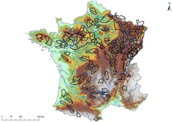
This study is based on a set of 211 catchments situated in France (Fig. 1). Meteorological and hydrological observed data are necessary for calibrating and running the hydrolog-ical model, as well as to evaluate the forecasts. For each catchment, time series of observed precipitation, daily mean

Fig. 1.Location of the 211 catchments studied in France.

evapotranspiration and discharge are available. Meteoro-logical data come from the meteoroMeteoro-logical analysis system SAFRAN of M´et´eo-France (Quintana-Segu´ı et al., 2008) for the period 1970 to 2006. The potential evapotranspiration was computed from temperature data using equations pro-posed by Oudin et al. (2005). Discharges come from the Banque Hydro (French database) and are available for a time period that varies according to each catchment, from 7 to 35 years, with 75% of the catchments with more than 27 years of data. Data were available at the daily time step.

2.2 Ensemble weather forecasts

The weather forecasts come from the meteorological ensem-ble prediction system PEARP of M´et´eo-France, based on the global spectral ARPEGE model (Nicolau, 2002). Initial per-turbations are generated by the singular vector technique and 11 future precipitation scenarios are proposed for each day of forecast. For this study, forecasts were provided with a 3-h time step, for a total forecast horizon of 60 h, at a 8-km×8-km grid resolution. Forecast data were aggregated at daily time steps to match the observed data and spatially averaged over the studied catchments (weighted mean using the surface of each grid cell inside the catchment) to obtain the areal forecast precipitation at each lead time (i.e., for 24 and 48 h ahead). Early assessments of the PEARP system have shown good skills for short-range prediction of severe events (Thirel et al., 2008; Randrianasolo et al., 2010), even if the system still shows a certain lack of spread.

2.3 Hydrological forecasting model: flow simulation and forecast updating

(3)

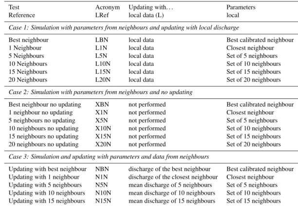
Table 1.Synthesis of the scenarios tested and the abbreviations used for each test.

Test Acronym Updating with. . . Parameters Reference LRef local data (L) local

Case 1: Simulation with parameters from neighbours and updating with local discharge

Best neighbour LBN local data Best calibrated neighbour 1 Neighbour L1N local data Closest neighbour 5 Neighbours L5N local data Set of 5 neighbours 10 Neighbours L10N local data Set of 10 neighbours 15 Neighbours L15N local data Set of 15 neighbours 20 Neighbours L20N local data Set of 20 neighbours

Case 2: Simulation with parameters from neighbours and no updating

Best neighbour no updating XBN not performed Best calibrated neighbour 1 neighbour no updating X1N not performed Closest neighbour 5 neighbours no updating X5N not performed Set of 5 neighbours 10 neighbours no updating X10N not performed Set of 10 neighbours 15 neighbours no updating X15N not performed Set of 15 neighbours 20 neighbours no updating X20N not performed Set of 20 neighbours

Case 3: Simulation and updating with parameters and data from neighbours

Updating with best neighbour NBN discharge of the best neighbour Best calibrated neighbour Updating with 1 neighbour N1N discharge of the closest neighbour Closest neighbour Updating with 5 neighbours N5N mean discharge of 5 neighbours Set of 5 neighbours Updating with 10 neighbours N10N mean discharge of 10 neighbours Set of 10 neighbours Updating with 15 neighbours N15N mean discharge of 15 neighbours Set of 15 neighbours Updating with 20 neighbours N20N mean discharge of 20 neighbours Set of 20 neighbours

Here, it is used at the daily time step. Input data are daily pre-cipitation and mean evapotranspiration.

Its mechanism is classic, with a production function, which confronts the daily amounts of rainfall and evapotran-spiration, and a routing function. It delays the release of ef-fective precipitation over the next time steps. This function includes a linear routing by a unit hydrograph and a non-linear one via a routing store, which transforms the effective rainfall into flow at the catchments outlet.

The GRP model has three parameters to be calibrated against observed data: the first one is a volume-adjustment factor, which acts over the volume of the effective rainfall, the second parameter is the maximum capacity of the rout-ing store and the last parameter is the base time of the unit hydrograph. Note that unlike the GR4J model from which it derives (Perrin et al., 2003), in GRP, the capacity of the SMA store is a fixed parameter. Finally, the forecasting model GRP uses a combination of two assimilation (updating) functions for flow forecasting. The first integrates the last observed dis-charge information at the time of the forecast to update the state of the model routing store, while the second uses the last observed forecast error to correct the forecasts (Berthet et al., 2009). Only the first updating is activated in the version of the model used in this study.

3 Methodology

The hydrological forecasting system used in this study con-sists of a rainfall-runoff simulation model and a proce-dure for forecast updating. For gauged catchments, model parametrization is made through a calibration procedure ap-plied to historic time series of concomitant precipitation and discharge observations. In real-time forecasting, the model also uses the last observed discharge (which usually differs from the last simulated discharge) in order to adjust the state of the routing store in the model in such a way that the output of the simulation agrees with the last observed discharge for the day preceding each day of forecast (for more details, see Berthet et al., 2009).

Thus, the use of the GRP hydrological forecasting model over ungauged catchments presents two challenges, which require transferring information from neighbour catchments: – first, to parameterize the model before launching the

forecasts;

(4)

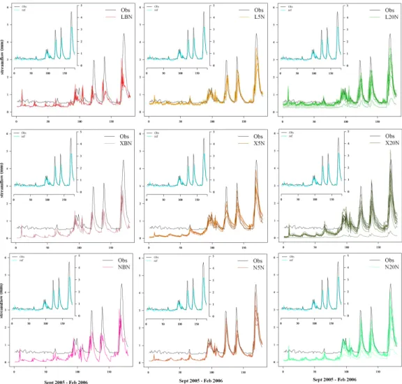
Fig. 2. Examples of predicted ensemble hydrographs for the catchment La Saˆone `a Auxonne (8900 km2)and 2 days of lead time. Top row: simulation with parameters from neighbour catchments and updating with local discharge. Middle row: simulation with parameters from neighbour catchments and no updating. Bottom row: simulation and updating with parameters and data from neighbour catchments. Neighbour catchments are: the best neighbour (left column; 11 members), the 5 (middle column; 55 members) and the 20 closest catchments (right column; 220 members). In each graphic, the reference scenario (11 members) is at the top left and the observed discharges are plotted.

3.1 Description of the different scenarios investigated

During the first step of the study, a reference situation, where local observed data were fully available, was simulated. For each catchment, the model was calibrated with historic local data and a set of optimal parameters was defined. This pa-rameter set was then applied during a forecasting period (in-dependent from the calibration period) and ensemble stream-flow forecasts were evaluated against observations. This sit-uation is supposed to give the best forecasts.

In the second step, a cross-validation approach was im-plemented: each catchment was considered as ungauged and evaluated in its turn. Different strategies for model parame-ter setup and forecast updating were investigated. Local data combined with data from neighbour catchments were used, as well as data from neighbour catchments alone. Proximity

of neighbours (also called “donors” using the common ter-minology of regionalization studies) was defined here by the Euclidean distanced, between the outlet of the ungauged site and the outlet of its neighbours (Eq. 1):

d= q

(Xtarget−Xneighbour)2+(Ytarget−Yneighbour)2, (1)

where Xtarget,Ytarget are the geographic coordinates of the

catchment considered as ungauged andXneighbour,Yneighbour

are the coordinates of the neighbour. On average, the closest neighbour and the 20-th farthest neighbour are about 2 km and 32 km, respectively, away from the target ungauged basin.

(5)

Case 1: Simulation with parameters from neighbours and updating with local discharge

This case corresponds to a situation where local discharge data start to be collected at the beginning of the forecast-ing period. This is a hypothetical situation where no his-toric data is available for model calibration and a gauging station is only put in place at the outlet of the catchment at the time the forecasting system starts to operate. In this case, local discharge data can only be used in forecast updating (the case is kept simple, and does not deal with a progres-sive recalibration of the model while data accumulate). Pa-rameter sets have to be transferred from gauged neighbour catchments to simulate streamflow ensembles. The alterna-tive scenarios use model parameters from 1, 5, 10, 15 and 20 nearest neighbour catchments. A scenario using the pa-rameter set from the neighbour catchment that gives the best performance during model calibration was also tested. On average, the best neighbour, which is among the 20 neigh-bours, is about 18 km away from the target ungauged basin.

Case 2: Simulation with parameters from neighbours and no updating

This case is similar to the previous one, except that here no local data are available at all: model parameters come either from the best neighbour catchment or from the nearest 1, 5, 15 and 20 neighbour catchments. No updating is used to correct the forecast in real-time.

Case 3: Simulation and updating with parameters and data from neighbours

Simulations at the target ungauged catchment are again based on model parameters transferred from the best bour catchment and from the nearest 1, 5, 15 and 20 neigh-bours. For the updating, a simple solution is tested, where the specific discharges from the neighbour catchments are used. For the best and the closest neighbour scenarios, their daily specific discharge observed prior to the day of forecast is used. For the multiple (5, 10, 15 and 20) neighbours sce-narios, the mean specific discharge observed at each neigh-bour site is transferred to the target site.

3.2 Calibration of the parameters of the “donor” catchments

Even if we test here the application of a flow forecasting model to ungauged catchments, this involves the use of donor catchments for which the hydrological model must have been calibrated previously. Thus, each catchment considered in turn as ungauged can benefit from a library of calibrated pa-rameter sets obtained from neighbouring gauged sites.

In calibration, the persistence index (Kitanidis and Bras, 1980) was used as objective function. It compares the pre-dictions of the model with the prediction obtained by assum-ing that the best estimate for the future is given by the latest discharge measurement. A description of the “step-by-step” global optimization procedure used here is given in Edijatno et al. (1999).

3.3 Evaluation of model ensemble forecasts

For each scenario, a streamflow ensemble is generated for each day of the forecasting period and for each forecast lead time, consisting of 11·N forecasts, whereN is the number of parameter sets (or neighbours) used to build the scenario. Therefore, for the scenario using the 5 nearest neighbours, an ensemble of 55 (11·5) members was obtained for each forecast, and so on for 10 (110 members), 15 (165 members) and 20 (220 members) neighbours.

Three general types of criteria can be found as the basis for the evaluation of forecasts (Murphy, 1993):

– consistency, when the forecaster’s best judgment and the forecast actually issued coincide,

– quality or accuracy, which considers the correspon-dence between the forecast and the observation, and – value, which concerns the economic worth of a forecast

to its user.

In this study, the quality of the ensemble streamflows ob-tained from each scenario tested was assessed. Forecast val-ues are compared to observed discharges over a 17-month period of forecast evaluation (from 10 March 2005 to 31 July 2006). Two lead times were considered: Day 1for the 24 h after the time the forecast is issued andDay 2, for the 24 h after Day 1, i.e., 48 h ahead the time of forecast. Typical scores of forecast performance were computed over the fore-cast evaluation period. They are summarized below and de-scribed in details in Jolliffe and Stephenson (2003):

– TheRMSE (root mean square error)measures the dis-tance between the forecasts and the observations and gives a measure of the forecast accuracy. Its advantage is being sensitive to large forecast errors and retaining the units of the forecast variable, thus being more easily interpretable as a typical error magnitude. The RMSE was calculated with the average streamflow forecast given by the ensemble mean of each scenario tested, for each lead time and over the total number of days of the evaluation period. To compare the scores over the 211 studied catchments, we computed normalized scores by dividing the RMSE of each catchment by its average observed streamflow over the evaluation period. – Thecontingency table is a two-dimensional table that

(6)

and “no” events. For the observed events, two stream-flow thresholds were defined for each catchment: the 50-th and the 90-th percentiles of daily streamflows, computed over the evaluation period (hereafter, Q50 andQ90, respectively). For the definition of forecasted events, two thresholds were selected: if p% of the ensemble members forecast discharges exceeding the streamflow threshold, the event is considered a ‘fore-casted event’. The values ofp% chosen in this study are 50% and 80% (hereafter,p50 and p80, respectively). The combination of these thresholds results in four con-tingency tables, from which descriptive statistics can be computed. A frequently used score, particularly when the non occurrence of the event is more frequent than its occurrence, is the Threat score (TS) or theCritical Success Index (CSI). It is given by the number of hits divided by the total number of hits, misses and false alarms. The worst possible score is 0 and the best is 1. – TheBrier score (BS) averages the squared differences

between pairs of forecast probabilities and the subse-quent binary observed frequencies of a given event (e.g., exceedance of a streamflow quantile). From Eq. (2), for each realizationj (here, day of forecast),yj is the fore-cast probability of the occurrence of the event, given by the ratio of ensemble members forecasting the event to the size of the ensemble, andoj= 1 if the event occurs and 0 if it does not occur:

BS= 1

N

n X

j=1

(yj−oj)2 (2)

The same streamflow thresholds used in the contingency ta-bles were considered to define an event: percentilesQ50 and

Q90. The Brier score is negatively oriented (smaller score better) and has a minimum value of 0 for a perfect (deter-ministic) system.

In order to compare the Brier score (BS) with a refer-ence (BSreference), it is convenient to define the Brier skill

score(BSS). The reference systems generally used are cli-matology and persistence. Here, since the aim is to evaluate the added value of alternative scenarios for ungauged catch-ments, comparatively to the reference situation where model calibration and updating are performed with local data, the scenario called “reference” (Table 1) is used to compute the BSreference. TheBSSungaugedis then given by:

BSSungauged=1−

BSscenario ungauged

BSreference gauged

(3)

TheBSSis positively oriented (higher values indicate better performance). It ranges from−∞to 1 (perfect deterministic system). Scores equal to 0 mean that the system does not give further information than the reference and negative scores in-dicate a poorer forecasting system than the reference.

– The Discrete ranked probability score (DRPS) is a squared measure that compares the cumulative density function of a probabilistic forecast with the cumulative density function of the corresponding observation over a given number of discrete probability categories (i.e., considering several streamflow thresholds). It is given by (Eq. 4):

DRPS=E[1

K

K X

j=1

(yj−oj)2], (4)

whereKis the number of categories of the distribution of the forecasts (here, defined by the thresholdsQ10,Q20,Q30,. . .

Q90 of streamflow quantiles),yj is the forecast probability for the category K andoj is the binary indicator for each categoryK(oj= 1 if the event occurs in theKcategory and 0, if not). The operatorEdenotes the average over the days of the forecasting period.

Like in theBS, skill scores were computed to compare the performance of the system given by each scenario tested with the reference scenario (DRPSS ungaugedderived from the

ap-plication of Eq. (3) to theDRPS).

4 Results

Figure 2 shows an example of hydrographs obtained for some of the different scenarios tested. The case of the Saˆone river at Auxonne (catchment area of 8900 km2)is illustrated for the reference scenario LRef (gauged catchment) and for the scenarios of ensemble predictions built from the best neigh-bour catchment, the 5 and the 20 nearest neighneigh-bours. The multiple simulations can be seen to get wider (more disper-sive) as the number of ensemble members increases. Addi-tionally, the forecast members ofCase 1(Fig. 2, top), where simulations are performed with parameters from neighbours and updating with local discharges, are closer to the observa-tion than the other forecasting scenarios considering the same number of neighbours. ForCase 2(simulations with param-eters from neighbours and no updating; Fig. 2, middle), a higher variability of forecast members is observed, compar-atively to the scenarios ofCase 3 (simulation and updating with parameters and data from neighbours; Fig. 2, bottom), for which the ensemble spread is low and the forecast mem-bers are farther from the observation. The hydrographs pre-sented in Fig. 2 correspond to one catchment and to a specific period in time (September 2005 to February 2006). Overall results from the scores used to evaluate the quality of the forecasts allow to better capture the average quality obtained for each scenario. They are presented in the next paragraphs for the lead timeDay 2.

4.1 Normalized RMSE andCSI_scores

(7)

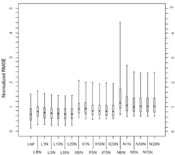
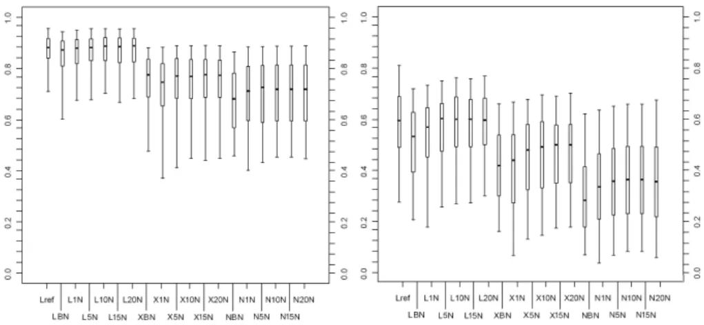
each scenario is presented in Fig. 4, for the ensemble thresh-oldp50 and for the streamflow thresholds ofQ50 andQ90 (also for a 2-day lead time). No significant differences were observed between the results with 50% and 80 % (not shown) of ensemble members exceeding the streamflow thresholds. This is probably due the lack of spread of the PEARP mem-bers, impacting the forecasts generated by the hydrological model (Randrianasolo et al., 2010). On the contrary, the CSI values decrease for the threshold Q90, comparatively to the values for the thresholdQ50, for all scenarios. For instance, for the reference scenario, the median values of CSI vary from 0.88 for Q50 to 0.69 forQ90. The perfor-mance for forecasting higher events is thus lower, although it has also to be considered that the number of events used in the computation of the scores is smaller. In general, for both RMSE and CSI scores, the ensemble scenarios built when updating is carried out with local discharges give bet-ter performance, with results closer to the reference situa-tion. The updating with specific discharges from neighbour catchments does not improve the forecasts. On the contrary, it gives the worst average performance. The performance for the non-updated forecast scenarios is between these two cases of updating tested (with local data and with data trans-ferred from neighbours). Small differences of performance are observed when using 1, 5, 10 and 20 neighbours, with a small improvement when increasing the number of neigh-bours. Distinctively, when comparing the results from the scenario based on the closest neighbour and the scenario based on the best neighbour (both scenarios have the same number of ensemble members), the results show that the for-mer surpasses more often the latter. The scenario with the best neighbour catchment as donor, regardless its proximity to the target catchment, has in most cases the worst median score value in each group of cases considered.

4.2 Skill scores

Figure 5 shows the skill scores of BSS andDRPSS when using the reference scenario as a reference forecast. The same conclusions as previously are obtained on the overall behaviour of the scores: the updating with local observations provides better performance (Case 1), the non-updated fore-casts present intermediate results (Case 2), and the updat-ing with data from neighbour catchments presents the lowest performance (Case 3). The scenarios that perform better are those when 5 to 20 neighbours are taken into account. It is interesting to note that, for more than 75% of the ungauged catchments, the gain is positive in the scenarios built with pa-rameters from 5 to 20 neighbours and updating based on lo-cal observations, showing that these scenarios give forecasts with higher skill, in a probabilistic way, than the reference forecast. Particularly for the non-updating case (scenarios fromCase 2), the average performance of the best neighbour is significantly better than the performance for the scenarios with 1, 5, 10, 15 and 20 closest neighbours. This is no longer

Fig. 3.Mean values of normalized RMSE for the reference and the scenarios tested (forecast lead time of 2 days and evaluation period from 10 March 2005 to 31 July 2006). Boxplots for the 211 studied catchments: the top and the bottom of the box represent the 75-th and the 25-th percentile, respectively, while the top and the bottom of the tail indicate the 95-th and the 5-th percentile, respectively. Median values are indicated.

the case when updating is performed with the average of spe-cific discharges from neighbours (scenarios fromCase 3), for which the closest neighbour performs on average better than the best neighbour. Moreover, for the skill scoreBSSungauged

and the Q50 threshold (Fig. 5, top), around 50% of the catch-ments give positive skill scores (better performance than the reference scenario), while the same is observed for around 25% of the catchments for theBSSungauged and the Q90%

threshold (Fig. 5, middle) and the DRPSSungauged (Fig. 5,

bottom).

4.3 Best scenario for each catchment

(8)

Fig. 4.Mean values ofCSIfor the reference and the scenarios tested (forecast lead time of 2 days and evaluation period from 10 March 2005 to 31 July 2006).CSIforp50 exceeding the discharge percentile Q50 (left) and Q90 (right). Boxplots for the 211 studied catchments: the top and the bottom of the box represent the 75-th and the 25-th percentile, respectively, while the top and the bottom of the tail indicate the 95-th and the 5-th percentile, respectively. Median values are indicated.

Fig. 5. Mean values of skill scores for the scenarios tested and relative to the reference scenario (forecast lead time of 2 days and evaluation period from 10 March 2005 to 31 July 2006). Top: BSS_ungaugedfor the discharge percentile Q50. Mid-dle: BSSungauged for the discharge percentile Q90. Bottom:

DRPSS_ungauged. Boxplots for the 211 studied catchments: the top and the bottom of the box represent the 75-th and the 25-th per-centile, respectively, while the top and the bottom of the tail indi-cate the 95th and the 5-th percentile, respectively. Median values are indicated.

of 211) are in this situation. They are particularly situated in the Eastern part of France, where the density of the studied catchments is more important. Considering the number of neighbours to be used when building the streamflow ensem-bles, the closest neighbour shows more often the best per-formance when focusing on the deterministic-based scores (RMSEandCSI). However, for the probabilistic-based scores (BSandDRPS), the scenarios that more often perform bet-ter are those when 5 to 20 neighbours are taken into account. Also, when focusing on large events, it is interesting to note that, for some catchments, the scenario that performs better becomes the scenario built with the best neighbour. This is noted when the results from theCSI andBSscores for the

Q90 threshold are analysed comparatively to the scores for theQ50 threshold. For the higher threshold, the best neigh-bour scenario shows up for 2 and 19 catchments for theBS and theCSIscore, respectively.

5 Conclusions

(9)

Fig. 6.Maps of the best performing scenario for each catchment according to the score:(a)RMSE,(b)CSIforp80 exceeding the discharge percentile Q50,(c)CSIforp80 exceeding the discharge percentileQ90,(d)BSfor the discharge percentile Q50,(e)BSfor the discharge percentileQ90, and(f)DRPS. Forecast lead time of 2 days and evaluation period from 10 March 2005 to 31 July 2006.

(i.e., historic and real-time data are available for model cal-ibration and forecast updating). Typical forecast perfor-mance measures were applied over a 17-month evaluation period. Both deterministic-focused measures (RMSE and CSI) and probabilistic-focused measures (BSSandDRPSS) were considered.

The results showed that the use of parameters from neigh-bour catchments can provide forecasts of good quality at the target ungauged site. This is particularly true when the trans-fer of parameters from gauged neighbours is accompanied by the implementation of a gauging station at the ungauged site, which provides local discharge information at the time of forecast for operational forecast updating. These scenar-ios, where the target site is considered partially ungauged (no historic data available for calibration, but data available at the time of forecast for updating of the system), are those that

most often show the performance that best approaches the performance of the reference gauged situation. Additionally, for these scenarios, in general, performance increases as the number of neighbours increases (from 1 to 20 neighbours as donors). This is particularly observed on the results from the probabilistic-based performance measures. The increase in spread of the streamflow ensemble predictions seems to have a positive effect on these performance measures.

(10)

general, lower median values of performance for the scenario that uses the best neighbour catchment (the catchment that showed better performance in calibration), the opposite is observed for the case when no updating is performed: the best neighbour scenario performs better than the 1 to 20 clos-est neighbour scenarios. It seems that in the non-updated case, the simulation part of the forecasting model prevails and, on average, better forecasts will be achieved when the system relies on parameters from the neighbour that gives the best model performance in calibration. On the contrary, when neighbour-based updating is performed, the updating component of the forecasting system is strengthened and it is rather the closest neighbours that will give better forecast performance.

In summary, this study illustrates well the added value of having at least local data available at the time of the forecast to perform the real-time updating of a hydrological ensem-ble forecasting system at sites where no historic data is avail-able for the set up (calibration) of the rainfall-runoff simula-tion model. For a better quality of the hydrological ensemble forecasts systems, if no local updating is possible, it is better to rely on the transfer of the parameters from the neighbour that showed best performance in calibration. If, in addition to model parameter transfer, neighbour-based updating is per-formed, the best solution is to rely on at least five closest neighbour donors.

Acknowledgements. We acknowledge the contribution of Météo-France, which gave us access to the SAFRAN data archive and to the PEARP ensemble forecasts, and the provision of the streamflow data by the MEEDM (Ministère de l’Ecologie, de l’Energie, du Développement durable et de la Mer).

Edited by: Y. He

Reviewed by: R. Turcotte and two other anonymous referees

References

Berthet, L., Andr´eassian, V., Perrin, C., and Javelle, P.: How cru-cial is it to account for the antecedent moisture conditions in flood forecasting? Comparison of event-based and continuous approaches on 178 catchments, Hydrol. Earth Syst. Sci., 13, 819– 831, doi:10.5194/hess-13-819-2009, 2009.

Cloke, H. L. and Pappenberger, F.: Ensemble flood forecasting: A review, J. Hydrol., 375, 613–626, 2009.

Edijatno, S., Nascimento, N., Yang, X., Makhlouf, Z., and Michel, C.: GR3J: a daily watershed model with three free parameters, Hydrolog. Sci. J., 44(2), 263–278, 1999.

Haché, M., Ouarda, T.B.M.J., Bruneau, P., and Bobée, B.: Es-timation régionale par la méthode de l’analyse canonique des corrélations: comparaison des types de variables hydrologiques. Can. J. Civil. Eng., 29, 899–910, 2002.

Jolliffe, I. T. and Stephenson D. B.: Forecast Verification. A Prac-titioner’s Guide in Atmospheric Science, John Wiley and Sons, Chichester, West Sussex, England, 240 pp., 2003.

Kay, A. L., Jones, D. A., Crooks, S. M., Calver, A., and Reynard, N. S.: A comparison of three approaches to spatial generalization of rainfall-runoff models, Hydrol. Process., 20, 3953–3973, 2007. Kitanidis, P. K. and Bras, R. L.: Real-time forecasting with a

con-ceptual hydrologic model 2. Applications and results, Water Re-sour. Res., 16, 1034–1044, 1980.

Kjeldsen, T. R. and Jones, D.: Estimation of an index flood using data transfer in the UK, Hydrolog. Sci. J., 52(1), 86–98, 2007. Kjeldsen, T. R. and Jones, D.: An exploratory analysis of error

components in hydrological regression modelling, Water Resour. Res., 45, W02407, doi:10.1029/2007WR006283, 2009. Kling, H. and Nachtnebel, H. P.: A method for the regional

estima-tion of runoff separaestima-tion parameters for hydrological modelling, J. Hydrol. , 364, 163–174, 2009.

Masih, I., Uhlenbrook, S., Maskey, S, and Ahmad, M. D.: Region-alization of a conceptual rainfall-runoff model based on similar-ity of the flow duration curve: A case study from the semi-arid Karkheh basin, Iran, J. Hydrol., 391, 188–201, 2010.

McIntyre, N., Lee, H., Wheater, H., Young, A., Wagener, T.: En-semble predictions of runoff in ungauged catchments, Water Re-sour. Res., 41, W12434, doi:10.1029/2005WR004289, 2005. Merz, R. and Bl¨oschl, G.: Regionalisation of catchment model

pa-rameters. J. Hydrol., 287, 95–123, 2004.

Murphy, A. H.: What is a good forecast? An essay on the nature of goodness in weather forecasting, Weather Forecast., 8, 281–293, 1993.

Nicolau, J.: Short-range ensemble forecasting. In Proceed-ings WMO/CBS Technical Conferences On Data Processing and Forecasting Systems, Cairns, Australia, 2–3 December, 4 pp., available at: http://www.wmo.ch/pages/prog/www/DPS/ TC-DPFS-2002/Papers-Posters/Topic1-Nicolau.pdf, 2002. Oudin, L., Hervieu, F., Michel, C., Perrin, C., Andr´eassian, V.,

An-ctil, F., and Loumagne, C.: Which potential evapotranspiration input for a lumped rainfall-runoff model? Part 2 – Towards a sim-ple and efficient potential evapotranspiration model for rainfall-runoff modelling, J. Hydrol., 303, 290–306, 2005.

Oudin, L., Andreassian, V., Perrin, C.,Michel, C., and Lemoine, N.: Spatial proximity, physical similarity, regression and ungauged catchments: A comparison of regionalization approaches based on 913 French catchments. Water Resour. Res., 44, W03413, doi:10.1029/2007WR006240, 2008.

Oudin, L., Kay, A. L., Andr´eassian, V., and Perrin, C.: Are seemingly physically similar catchments truly hy-drologically similar?, Water Resour. Res., 46, W11558, doi:10.1029/2009WR008887, 2011.

Ouarda, T., Ba, K. M., Diaz-Delgado, C., Carsteanu A., Chokmani, K., Gingras, H., Quentin, E., Trujillo, E., and Bob´ee, B.: Inter-comparison of regional flood frequency estimation methods at ungauged sites for a Mexican case study, J. Hydrol., 348, 40–58, 2007.

Parajka, J., Merz, R., and Bl¨oschl, G.: A comparison of regional-isation methods for catchment model parameters, Hydrol. Earth Syst. Sci., 9, 157–171, doi:10.5194/hess-9-157-2005, 2005. Perrin, C., Michel, C., and Andr´eassian, V.: Improvement of a

parsi-monious model for streamflow simulation, J. Hydrol., 279, 275– 289, 2003.

(11)

SAFRAN analysis over France, J. Appl. Meteorol. Clim., 47(1), 92–107, 2008.

Randrianasolo, A., Ramos, M.-H., Thirel, G., Andr´eassian V., and Martin, E.: Comparing the scores of hydrological ensemble fore-casts issued by two different hydrological models, Atmos. Sci. Lett., 11(2), 100–107, 2010.

Reichl, J. P. C., Western, A. W., McIntyre, N. R., and Chiew, F. H. S.: Optimization of a similarity measure for estimat-ing ungauged streamflow, Water Resour. Res., 45, W10423, doi:10.1029/2008WR007248, 2009.

Sivapalan, M., Takeuchi, K., Franks, S. W., Gupta, V. K., Karam-biri, H., Lakshmi, V., Liang, X., McDonnell, J. J., Mendiodo,

E. M., O’Connell, P. E., Oki, T., Pomeroy, J. W., Schertzer, D., Uhlenbrook, S., and Zehe, E.: IAHS decade on prediction in ungauged basins (PUB), 2003–2012: shaping an exciting future for the hydrological sciences, J. Hydrolog. Sci., 48(6), 857–880, 2003.

Thirel, G., Rousset-Regimbeau, F., Martin, E., and Habets, F.: On the impact of short-range meteorological forecasts for ensemble streamflow prediction, J. Hydrometeorol., 9, 1301–1317, 2008. Young, A. R.: Streamflow simulation within UK ungauged