2CERENA, Instituto Superior T´ecnico, Lisbon, Portugal
Received: 4 March 2008 – Revised: 27 June 2008 – Accepted: 3 July 2008 – Published: 30 July 2008
Abstract. The topographic characteristics and spatial cli-matic diversity are significant in the South of continental Por-tugal where the rainfall regime is typically Mediterranean. Direct sequential cosimulation is proposed for mapping an extreme precipitation index in southern Portugal using eleva-tion as auxiliary informaeleva-tion. The analysed index (R5D) can be considered a flood indicator because it provides a measure of medium-term precipitation total. The methodology ac-counts for local data variability and incorporates space-time models that allow capturing long-term trends of extreme pre-cipitation, and local changes in the relationship between ele-vation and extreme precipitation through time. Annual grid-ded datasets of the flood indicator are produced from 1940 to 1999 on 800 m×800 m grids by using the space-time rela-tionship between elevation and the index. Uncertainty eval-uations of the proposed scenarios are also produced for each year. The results indicate that the relationship between el-evation and extreme precipitation varies locally and has de-creased through time over the study region. In wetter years the flood indicator exhibits the highest values in mountainous regions of the South, while in drier years the spatial pattern of extreme precipitation has much less variability over the study region. The uncertainty of extreme precipitation esti-mates also varies in time and space, and in earlier decades is strongly dependent on the density of the monitoring stations network. The produced maps will be useful in regional and local studies related to climate change, desertification, land and water resources management, hydrological modelling, and flood mitigation planning.
Correspondence to: A. C. Costa ([email protected])
1 Introduction
Information on the spatial variability of extreme precipita-tion is important for river basins management, flood hazards protection, studies related to climate change, erosion elling and other applications for hydrological impact mod-elling. It is long recognized that topography and other geo-graphical factors are responsible for considerable spatial het-erogeneity of the precipitation distribution at the sub-regional scale (e.g., Mart´ınez-Cob, 1996; Daly, 2006). A comprehen-sive review on the complex relationship between precipita-tion, airflow and physiographic features of mountainous re-gions is presented by Johansson and Chen (2003), and Smith and Barstad (2004). Accordingly, it is commonly accepted that interpolation techniques that make use of the relation-ship between existing station data and explanatory physio-graphic variables (e.g., elevation or distance to the coast-line) have the potential to better represent the actual climate spatial patterns, especially in mountainous areas and in re-gions with complex atmospheric influences (Prudhomme and Reed, 1998; Daly, 2006).
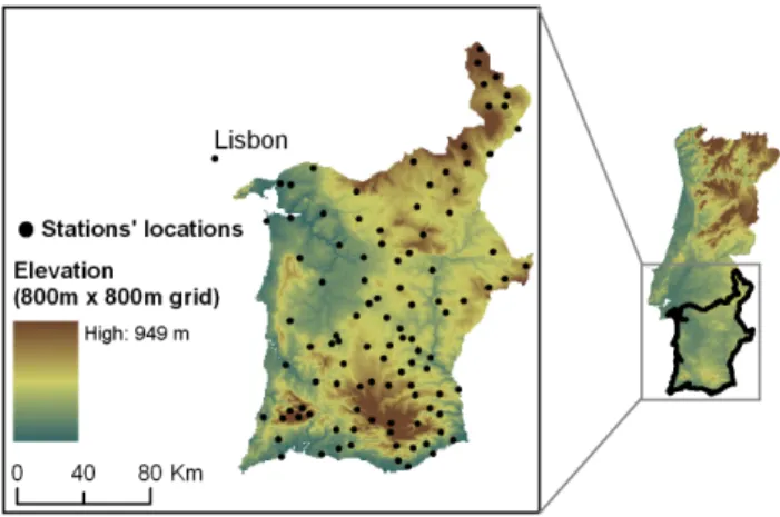
Fig. 1. Elevation of the study region in the South of Portugal and
stations’ locations.
The number of studies on the interpolation of extreme pre-cipitation indicators is limited. The works of Faulkner and Prudhomme (1998) and Prudhomme and Reed (1998, 1999) focused on an index of extreme rainfall, named RMED – me-dian of the annual maximum rainfall, while Hundecha and B´ardossy (2005) and Perry and Hollis (2005) describe the mapping of several extreme precipitation indices. Faulkner and Prudhomme (1998), Prudhomme and Reed (1999), and Perry and Hollis (2005) used techniques that combine dis-tance weighting methods and regression to produce gridded datasets of extreme precipitation indices, whereas Hundecha and B´ardossy (2005) used kriging with external drift to inter-polate daily precipitation observations on a 5 km×5 km grid and calculated the extreme precipitation indices, afterwards, on derived grids of 5, 10, 25 and 50 km2. Interpolation usually leads to a smoothing of the distribution inferred by the observations and thus to a loss of variance. For exam-ple, it is well known that kriging is locally accurate in the minimum error variance sense, but does not provide repre-sentations of spatial variability given the “smoothing” effect of kriging (Goovaerts, 1997). The smoothing effect in pre-cipitation data is undesirable considering the modelling of floods or other extreme hydrological processes (Haberlandt, 2007). To overcome this limitation, geostatistical stochas-tic simulation has become a widely accepted procedure to reproduce the spatial distribution and uncertainty of highly variable phenomena in geosciences (e.g., Franco et al., 2006; Bourennane et al., 2007). Geostatistical simulation methods describe local data variability based on many, equally proba-ble, realizations of the phenomenon, consistent with the data and its statistical characteristics.
The accuracy and uncertainty of gridded data sets is dif-ficult to assess because the field that is being estimated is unknown between data points. Spatial interpolation errors are interdependent functions of the station-network distribu-tion, the efficacy of the interpolation procedure, and the real (but unknown) spatial distribution of the underlying climatic
Fig. 2. Distribution of the number of available stations by year.
field (Willmott and Matsuura, 2006). Unlike traditional in-terpolation methods (e.g., cokriging), geostatistical simula-tion procedures aim at reproducing the spatial uncertainty of the attribute under study. The series of simulated maps can be post-processed and the spatial uncertainty summarized (Goovaerts, 1997). For example, the uncertainty at an un-sampled location can be evaluated through spread measures, such as the variance, derived from the corresponding local histogram.
As other southern European regions, the rainfall regime in southern Portugal is Mediterranean, and so highly vari-able in both the spatial and temporal dimensions. One par-ticularly relevant feature of the rainfall regime in this area is the occurrence of short but very intensive rainfall events that may lead to significant damages, by causing flash floods that affect small drainage basins (Ramos and Reis, 2002). Fragoso and Gomes (2008) concluded that the most southern region (Algarve) is the one where episodes of heavy rainfall are most frequent and which exhibits the strongest torrential character.
In this work, the R5D index was chosen to characterize the extreme precipitation regime. This indicator is defined as the highest consecutive 5-day precipitation total (in millimetres) per year, and so provides a measure of medium-term precipi-tation total. For the interpolation and uncertainty assessment of extreme precipitation in the southern region of continen-tal Portugal, we explore the application of direct sequential cosimulation, which allows incorporating covariates such as elevation.
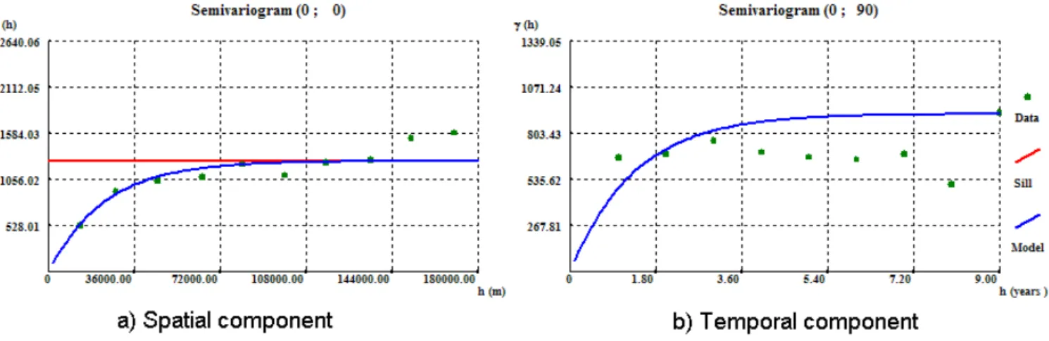
Fig. 3. Spatial and temporal components of the experimental semivariogram of the 1960s decade data of R5D with the exponential model
fitted.
detected in southern Portugal (Corte-Real et al., 1998). Ac-cordingly, the methodology not only accounts for local data variability by using stochastic simulation procedures, but also incorporates space-time models that allow capturing long-term trends of extreme precipitation, and local corre-lations between elevation and precipitation through time.
The current work has three objectives: (i) to assess the space-time relationship between elevation and extreme pre-cipitation in southern Portugal; (ii) to use this relationship to produce annual gridded datasets of a flood indicator (R5D) from 1940 to 1999; and (iii) to provide an uncertainty evalu-ation of the produced scenarios.
The R5D index was computed using high quality daily pre-cipitation observations measured at 105 monitoring stations with data within the period 1940/1999. The direct sequen-tial cosimulation was performed for generating one map per year, using 800 m×800 m grids and elevation as exhaustive secondary information.
The methodology is briefly introduced in Sect. 2, and the study region and data are described in Sect. 3. The main results are presented and discussed in Sect. 4, including the relationship between elevation and the flood indicator, the space-time patterns of the index in 1940/1999, and the un-certainty evaluation of the produced maps. Finally, Sect. 5 states the major conclusions.
2 Methods
This section briefly introduces the kriging techniques and de-scribes the reasoning of the geostatistical stochastic simula-tion algorithms implemented. Interested readers should refer to geostatistical textbooks (e.g., Isaaks and Srivastava, 1989; Goovaerts, 1997) for detailed descriptions of univariate and multivariate geostatistical methods. For a thorough descrip-tion of the direct sequential simuladescrip-tion, and cosimuladescrip-tion, al-gorithms the reader is referred to Soares (2001).
Geostatistical estimators, known as kriging, provide sta-tistically unbiased estimates of surface values from a set of observations at recorded locations, using the estimated spa-tial (and temporal) covariance model of the observed data.
Consider the two dimensional problem of estimating a pri-mary variable zat an unsampled location u0. Let {z(uα),
α=1, . . . ,n}be the set of primary data measured atn loca-tions uα. Most of geostatistics is based on the assumption
that the set of unknown values is a set of spatially dependent random variables, hence each measurementz(uα)is a
partic-ular realization of the random variableZ(uα). Kriging uses a
linear combination of neighbouring observations to estimate the unknown value at the unsampled locationu0. This
prob-lem can be expressed in terms of random variables as: ˆ
Z (u0)= n
X
α=1
λαZ (uα). (1)
The optimal kriging weightsλα are determined by solving
the kriging equations that result from minimizing the estima-tion variance while ensuring unbiased estimaestima-tion of Z(u0)
byZ (uˆ 0).
Kriging methods require a stationarity assumption, ex-pressed in two parts. First, the mean of the process is as-sumed constant and invariant with spatial location (first order stationarity). Second, the variance of the difference between two values is assumed to depend only on the distanceh be-tween the two points, and not on their location u (second order stationarity). Stationarity assumptions on kriging are traditionally accounted for by using local search neighbour-hoods so that the dependence on stationarity becomes local (Goovaerts, 1997).
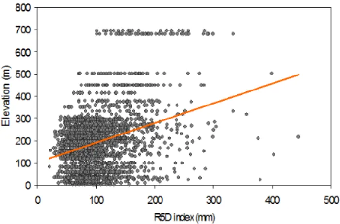
Fig. 4. Plot of elevation against R5D values calculated within 1940/99.
mathematical variogram model is selected from a small set of authorised ones (e.g. exponential or spherical) and is fitted to experimental semivariogram values calculated from data for given angular and distance classes.
The experimental semivariogramγ (h)ˆ is computed as half the average squared difference between data pairs belonging to a certain angular and distance class:
ˆ
γ (h)= 1 2N (h)
N (h)X
α=1
[z(uα)−z(uα+h)]2 (2)
whereN (h)is the number of pairs of data locations a vec-torhapart.
In bounded models (e.g., spherical and exponential), var-iogram functions increase with distance until they reach a maximum, named sill, at an approximate distance known as the range. The range is the distancehat which the spatial (or temporal) correlation vanishes, i.e. observations separated by a distance larger than the range are spatially (or temporally) independent observations.
2.1 Simple kriging
The simple kriging estimate ofz(u0)is:
ˆ
zSK(u0)−m= n(u)
X
α=1
λSKα (u0)[z(uα)−m] (3)
wheremis the stationary mean ofZ(u), andλSKα (u0)is
the weight assigned to datumz(uα)within a search
neigh-bourhood that comprisesn(u)samples.
Fig. 5. Regional correlation between elevation and R5D values by
year.
2.2 Collocated cokriging
Consider now the situation where the set of primary data {z(uα), α=1, . . . , n} is complemented by secondary data
available at all estimation grid nodes and denoted byy(u). The collocated cokriging estimate is (Goovaerts, 2000):
ˆ
zCoK(u0)= n(u) X
α=1
λCoKα (u0) z (uα)+λCoK(u0)[y (u0)−mY+mZ] (4) wheremZandmY are the global means of the primary and
secondary variables,Z(u)andY (u), respectively. Note that only the secondary datum collocated at the locationu0being
estimated is retained for estimation. 2.3 Direct sequential cosimulation
Soares (2001) describes the sequence of the direct sequen-tial simulation (DSS) algorithm of a continuous variable as follows:
1. Randomly select the spatial location of a nodez(u0)in
a regular grid of nodes to be simulated;
2. Estimate local mean and variance identified with simple kriging estimator (Eq. 3) and kriging variance. Sample from the global histogram a valuezs(ui)centred in the
estimated local mean and variance.
3. Return to step 1) until all nodes have been visited by the random path.
Soares (2001) also extended the DSS algorithm for the joint simulation of different variables, thus named direct se-quential cosimulation (coDSS) algorithm. Instead of simu-lating all variables simultaneously, it simulates each variable in turn conditioned to the previous simulated variable.
Fig. 6. Local correlation models between elevation and R5D values
for each decade.
variable variogram model and a correlation model between primary and secondary data were required.
To reproduce the spatial distribution and uncertainty of the flood indicator, 100 equiprobable simulated realizations were generated through the coDSS algorithm on 800 m×800 m grids, one for each year, using different space-time continu-ity and correlation models for each decade. These models are briefly described in the following section and further detailed in Sect. 4. Elevation was used as secondary information. 2.4 Space-time continuity models
Simulated images were generated by the coDSS algorithm using for each decade a different space-time variogram model of the primary variable (R5D index), and a differ-ent correlation model between primary and exhaustive sec-ondary data (elevation). This strategy allows accounting for
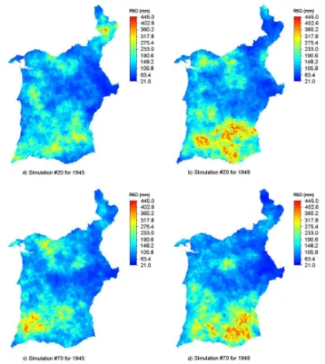
Fig. 7. Equiprobable simulated realizations of R5D for 1945 and
1949.
possible long-term trends or fluctuations in extreme rainfall, and for changes in the relationship between elevation and ex-treme precipitation through time. Alternative physiographic variables, such as slope or distance from the coastline, could have been used as secondary information.
The relationship between elevation and extreme precipi-tation, described by correlation models, was also assessed locally to allow accounting for changes in correlation across the study area. First, for each decade, local correlations were calculated using a search neighbourhood centred at each sta-tion’s location (further details from this stage are described in Sect. 4.2). To reproduce the spatial distribution of the re-lationship between elevation and extreme precipitation, the second stage used the DSS algorithm to interpolate the local correlations. In this stage, 50 equiprobable simulated real-izations were generated through the DSS algorithm for each decade on 800 m×800 m grids. The correlation models used later with the coDSS algorithm were determined by comput-ing the mean of the distribution of the 50 simulated values at each grid node, by decade.
3 Study region and data
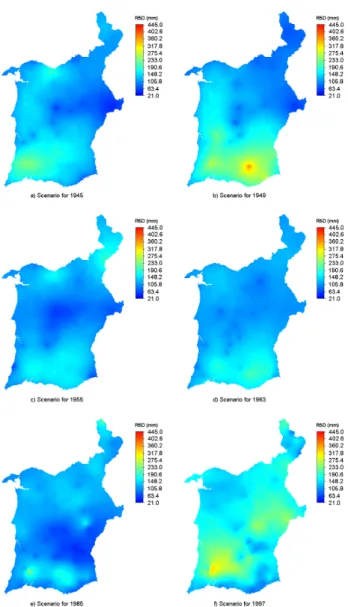
Fig. 8. Scenarios of extreme precipitation (R5D index).
characteristics. In the far South, the relief is dominated by the two main Algarve’s mountains: Monchique on the West, and Caldeir˜ao on the East. In contrast, the Alentejo region is characterized mainly by vast flat to rolling country, the pene-plain, where the average altitude is approximately 200 m. The S˜ao Mamede mountain ridge, the highest in the Alen-tejo region with an altitude of 1000 m, lies in the extreme North-East.
Daily rainfall series from 105 stations distributed irregu-larly over the study region were collected (Fig. 1). Most of them were extracted from the National System of Wa-ter Resources Information (SNIRH – Sistema Nacional de Informac¸˜ao de Recursos H´ıdricos) database (http://snirh. inag.pt), and three of them were compiled from the Euro-pean Climate Assessment dataset (http://eca.knmi.nl). Each station series data was previously quality controlled and stud-ied for homogeneity (e.g. Wijngaard et al., 2003; Costa and
Table 1. Parameters of the exponential variogram models for the
R5D index, by decade.
Decade Spatial range (m) Temporal range Sill (years)
1940/49 85 000 4.5 2923.364
1950/59 100 000 1 2075.247
1960/69 70 000 4 1263.25
1970/79 70 000 5 1543.205
1980/89 150 000 4.5 2075.301
1990/99 165 000 1.3 2803.646
Soares, 2006; Costa et al., 2008). The length of the series is highly variable. The extreme precipitation index (R5D) was calculated for each station using all quality data avail-able within the 1940/99 period (Fig. 2). The selected stations have less than 16% of the days missing in each year and most stations’ data do not have any missing records. The R5D in-dex is defined as the highest consecutive 5-day precipitation total (in millimetres) per year, and can be considered a flood indicator (Frich et al., 2002).
Elevation data were taken from a digital elevation model (DEM) with a grid resolution of 20 m×20 m and resampled to an 800 m×800 m grid mesh. The topographic variable de-rived is defined as the elevation of the nearest grid point to the meteorological station location, sometimes named smoothed elevation.
4 Results and discussion
4.1 Space-time continuity of extreme precipitation Variograms were calculated according to Eq. 2. The vari-ogram models are chosen and their parameters are estimated taking into account the experimental data values of vari-ograms. The objective is to capture the spatial pattern of physical phenomenon in the variogram model rather than getting a best fit of a second moment (Goovaerts, 1997). In this study, we chose exponential models that capture the ma-jor spatial features of the attribute under study within each decade. The selected models were subjectively fitted to the experimental semivariogram values, not only by giving more importance to the smaller lags and the ones computed from more data pairs, but also by taking into account physical knowledge of the area and phenomenon. Considering the re-sults of a thorough analysis on directional variograms, only the omnidirectional semivariograms for the spatial dimen-sion were retained. Consequently, the spatial variability is assumed to be identical in all directions (i.e. isotropic) within each decade.
spatial component shows a strong increase in the spatial con-tinuity of the flood indicator on the last two decades. For illustration purposes, the exponential model fitted to the ex-perimental semivariogram of the 1960s decade is shown in Fig. 3.
4.2 Relationship between extreme precipitation and eleva-tion
An exploratory evaluation of the relationship between the ex-treme precipitation index and elevation was made by aver-aging the R5D index at each station, and by computing af-terwards the Pearson’s correlation coefficient between those values and elevation, not only measured by the actual sta-tions altitude, but also by the stasta-tions grid point elevation (smoothed elevation). This regional analysis shows that the correlation is slightly stronger for the smoothed elevation (0.49) than the actual one (0.43). Other studies on this sub-ject concluded likewise (e.g., Diodato, 2005).
A plot of elevation against R5D index values is given in Fig. 4. The coefficient of determination,r2, is small (0.10) and so there is little evidence of a (global) linear relationship between elevation and precipitation, as expected (e.g., Lloyd, 2005). Moreover, the correlation for elevation against R5D index values is not constant through time (Fig. 5), but rather shows a negative trend during the study period, although not statistically significant. The number of stations used in the computation of these correlations ranges from 19 (in 1940) to 93 (in 1991 and 1992), and is always less than 40 before 1980. Because of the sparse coverage of meteorological sta-tions in some areas, especially until the 1980s decade (Ta-ble 2), the local relationship between elevation and extreme precipitation was assessed by decade.
The coDSS algorithm uses a different correlation model between the R5D index and elevation within each decade. In order to determine these models, first, the relationship be-tween elevation and precipitation was assessed locally by computing, for each decade, Pearson’s correlation coeffi-cients using stations’ data falling within a circle centred at each station’s location. As in earlier decades meteorological stations are scarce, larger radii were used (Table 2).
Sec-Fig. 9. Uncertainty of the scenarios of extreme precipitation (R5D
index).
ond, the DSS algorithm was applied to interpolate the lo-cal correlations by decade. This procedure used a single space-time spherical variogram model of the local correla-tions, where the spatial dimension was modelled as isotropic, the estimated range of the spatial dimension was 110 000 m, the range of the temporal dimension was 6 decades, and the estimated sill was 0.053. Finally, the correlation models were determined by computing the mean of the distribution of 50 simulated values at each grid node, by decade (Fig. 6).
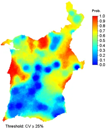
Fig. 10. Probability of the uncertainty of the R5D index scenarios,
measured by the coefficient of variation, to be greater than or equal to 25%.
stations. Accordingly, the variability associated with esti-mated correlations over this area is also high. Nevertheless, they correspond to moderate values of approximately 0.50, and so the contribution of elevation to the estimation of the flood indicator will also be moderate. The correlation model of the 1950s decade exhibits a more realistic pattern, with correlations ranging from−0.17 to 0.67. The model of the 1960s decade also shows a realistic pattern of correlations, although the West and North-East areas present high vari-ability. Similarly, the 1970s decade model is realistic but with very high variability within the North-East region. Be-cause of the higher density of stations, the correlation models of the 1980s and 1990s decades exhibit much less variability than the previous ones.
These results suggest that using elevation as a secondary variable in estimation will increase the accuracy of estimates in some locations, i.e. those mountainous areas where cor-relations are large (e.g. on the West of Algarve and on the North-East of the study region). In contrast, univariate in-terpolators (e.g., DSS) are likely to provide estimates as ac-curate as those provided by coDSS, with less computational effort, in places where correlations are small.
4.3 Extreme precipitation scenarios
Using the coDSS algorithm, a set of 100 equiprobable sim-ulated realizations of the R5D index was computed at each simulated grid node, by year. For illustration purposes, two equiprobable realizations, for 1945 and 1949, are shown in Fig. 7. The space-time inference was performed by means of computing the mean of those distributions. Uncertainty was assessed by means of computing the standard-deviation (STD) and the coefficient of variation (CV) of the distribu-tion of the 100 simulated values at each simulated grid node, by year. For illustration purposes, the flood indicator maps of six years are shown in Fig. 8, while Fig. 9 presents their un-certainty evaluation measured by the coefficient of variation (CV).
Although the correlation model for the 1940s decade seemed unrealistic, a visual inspection of all produced sce-narios for those years reveals a rather realistic spatial pat-tern of extreme precipitation. On the other hand, the lack of precipitation data on the north-eastern area makes the esti-mates more uncertain. For that reason, the extreme precipita-tion values were possibly less accurately estimated over that area in several years. In fact, as expected, one of the regions where the distribution of extreme precipitation shows greater variability, thus more uncertainty, is in the northern part of the maps, corresponding to regions less densely sampled in most years. This is especially evident in the maps of the standard-deviation. Moreover, the scenarios for the last two decades of the twentieth century show less uncertainty than the previous ones because the availability of stations over the study region is considerably greater (Fig. 2).
Fig. 10 shows estimated local probabilities of the coeffi-cient of variation of the scenarios produced for R5D to be greater than or equal to 25%. These probabilities were eval-uated as the proportion of the sixty estimated values of CV (computed at each grid cell throughout the years) that exceed that threshold.
Only a few stations are located at medium (>400 m) and high elevations (Table 2), thus greater uncertainty would be expected at those regions. However, the uncertainty in the mountainous regions of the South is often small (Fig. 10), because of the use of elevation as secondary exhaustive in-formation in the spatial interpolation procedure of R5D.
(NAO) are likely to be responsible for much of the observed change in the frequency of above 90th percentile winter pre-cipitation between the 1960s and 1990s over Europe (Scaife et al., 2008). Moreover, the NAO–rainfall relationships tend to be stronger during the wet seasons of the last decades of the twentieth century in southern Portugal (Goodess and Jones, 2002; Trigo et al., 2004). Accordingly, changes in the NAO are likely to be responsible for the increase of the spatial continuity of R5D in southern Portugal, which is es-pecially pronounced during the last two decades of the twen-tieth century.
To illustrate the usefulness of the annual gridded datasets produced for the R5D index, probability maps of extreme precipitation were computed as follows. First, the regional histogram and its basic statistics were calculated using the R5D values from maps corresponding to the climate normal 1961/1990. For example, the median was equal to 105 mm, the third quartile was 125 mm, and the 95th percentile was 160 mm. Second, the probability is approximated by the rel-ative frequency computed at each grid node for 1940/1999. Frequencies correspond to the number of times that R5D values are equal or over a fixed threshold. For example, the probability map corresponding to the 105 mm threshold (Fig. 11) shows that the mountainous regions of Algarve and North-East, and also the West coast have high probability of extreme rainfall events. On the other hand, the probability map for 125 mm (Fig. 11) shows that the heaviest medium-term rainfall events occur at the Algarve region, especially over the Monchique mountains, as expected. Probability maps such as these might be useful to identify regions at risk of erosion caused by extreme precipitation events.
5 Conclusions
The study was performed in the South of continental Portugal where the topographic characteristics and spatial climatic di-versity are significant, although the region’s relief is not very complex if compared to other European study regions (e.g., Prudhomme and Reed, 1999; Perry and Hollis, 2005). The correlation maps of elevation and R5D values indicate that, as the relationship varies locally, the benefits in using
eleva-tion data to inform estimaeleva-tion will also vary locally. There-fore, using elevation data in the estimation process is likely to be beneficial, especially in mountainous areas. The esti-mates accuracy also varies in time, and in earlier decades is strongly dependent on the density of the stations network.
Nevertheless, the flood indicator values at locations be-tween meteorological stations have been estimated to a good degree of accuracy in most years, producing detailed and rep-resentative maps of extreme precipitation space-time patterns over the South of Portugal for the 1940/1999 period. There-fore, the produced gridded datasets provide a consistent set of data that allows further investigations on the spatial and temporal variability and trends in the South Portugal climate, over 60 years. In fact, the usefulness of the datasets was il-lustrated by probability maps of extreme precipitation.
The methodology considered here has clear theoretical ad-vantages over alternative ones, although no single method is optimal for all regions and time periods (e.g., Isaaks and Srivastava, 1989; Lloyd, 2005). Among the sequential al-gorithms of stochastic simulation, one advantage of direct sequential simulation and cosimulation is the use of original variables instead of transformed ones: Gaussian (sequential Gaussian simulation) or indicator (sequential indicator sim-ulation). The direct sequential cosimulation proved to be a valuable technique to deepen the knowledge on the space-time patterns of extreme precipitation over the study domain, because it allowed incorporating elevation information into prediction and also used all quality data available for every station. Furthermore, this approach accounted for local data variability and made possible uncertainty evaluations of the proposed scenarios.
Acknowledgements. This research was developed in the
(Programme Interreg IIIB, MEDDOC, convention no. 2005-05-4.4-P-105).
The authors also thank two anonymous reviewers for valuable suggestions, which helped them to improve the quality of this paper.
Edited by: A. Mugnai and A. Bartzokas Reviewed by: two anonymous referees
References
Boer, E. P. J, de Beurs, K. M., and Hartkamp, A. D.: Kriging and thin plate splines for mapping climate variables, Int. J. Appl. Earth Obs., 3(2), 146–154, 2001.
Bourennane, H., King, D., Couturier, A., Nicoullaud, B., Mary, B., and Richard, G.: Uncertainty assessment of soil water content spatial patterns using geostatistical simulations: An empirical comparison of a simulation accounting for single attribute and a simulation accounting for secondary information, Ecol. Model., 205, 323–335, 2007.
Brunsdon, C., Mcclatchey, J., and Unwin, D. J.: Spatial variations in the average rainfall-altitude relationship in Great Britain: an approach using geographically weighted regression, Int. J. Cli-matol., 21, 4, 455–466, 2001.
Corte-Real, J., Qian, B., and Xu, H.: Regional climate change in Portugal: precipitation variability associated with large-scale at-mospheric circulation, Int. J. Climatol., 18, 619–635, 1998. Costa, A. C. and Soares, A.: Identification of inhomogeneities in
precipitation time series using SUR models and the Ellipse test, in: Proceedings of Accuracy 2006 – 7th International Sympo-sium on Spatial Accuracy Assessment in Natural Resources and Environmental Sciences, edited by: Caetano, M. and Painho, M., Instituto Geogr´afico Portuguˆes, 419–428, 2006.
Costa, A. C., Negreiros, J., and Soares, A.: Identification of inho-mogeneities in precipitation time series using stochastic simula-tion, in: geoENV VI – Geostatistics for Environmental Applica-tions, edited by: Soares, A., Pereira, M. J., and Dimitrakopoulos, R., Springer, 15, 275–282, 2008.
Cubasch, U., von Storch, H., Waszkewitz, J., and Zorita, E.: Es-timates of climate change in Southern Europe derived from dy-namical climate model output, Clim. Res., 7, 129–149, 1996. Daly, C., Neilson, R. P., and Phillips, D. L.: A
statistical-topographic model for mapping climatological precipitation over mountainous terrain, J. Appl. Meteorol., 33, 140–157, 1994. Daly, C.: Guidelines for assessing the suitability of spatial climate
data sets, Int. J. Climatol., 26(6), 707–721, 2006.
Diodato, N.: The influence of topographic co-variables on the spa-tial variability of precipitation over small regions of complex ter-rain, Int. J. Climatol., 25(3), 351–363, 2005.
Faulkner, D. S. and Prudhomme, C.: Mapping an index of extreme rainfall across the UK, Hydrol. Earth Syst. Sc., 2, 183–194, 1998. Fragoso, M. and Gomes, P. T.: Classification of daily abundant rainfall patterns and associated large-scale atmospheric circula-tion types in Southern Portugal, Int. J. Climatol., 28(4), 537–544, doi:10.1002/joc.1564, 2008.
Franco, C., Soares, A., and Delgado, J.: Geostatistical modelling of heavy metal contamination in the topsoil of Guadiamar river margins (S Spain) using a stochastic simulation technique, Geo-derma, 136, 852–864, 2006.
Frich, P., Alexander, L. V., Della-Marta, P., Gleason, B., Haylock, M., Klein Tank, A. M. G., and Peterson, T.: Observed coherent changes in climatic extremes during the second half of the twen-tieth century, Climate Res., 19(3), 193–212, 2002.
Goodess, C. M. and Jones, P. D.: Links between circulation and changes in the characteristics of Iberian rainfall, Int. J. Climatol., 22(13), 1593–1615, 2002.
Goovaerts, P.: Geostatistics for Natural Resources Evaluation. Ap-plied Geostatistics Series, Oxford University Press, New York, Oxford, 1997.
Goovaerts, P.: Geostatistical approaches for incorporating elevation into the spatial interpolation of rainfall, J. Hydrol., 228, 113–129, 2000.
Haberlandt, U.: Geostatistical interpolation of hourly precipitation from rain gauges and radar for a large-scale extreme rainfall event, J. Hydrol., 332, 144–157, 2007.
Hundecha, Y. and B´ardossy, A.: Trends in daily precipitation and temperature extremes across western Germany in the second half of the 20th century, Int. J. Climatol., 25(9), 1189–1202, 2005. Hutchinson, M. F.: Interpolating mean rainfall using thin plate
smoothing splines, Int. J. Geogr. Inf. Syst., 9, 385–403, 1995. Isaaks, E. H. and Srivastava, R. M.: An Introduction to Applied
Geostatistics, Oxford University Press, New York, Oxford, 1989. Johansson, B. and Chen, D.: The influence of wind and topography on precipitation distribution in Sweden: statistical analysis and modelling, Int. J. Climatol., 23(12), 1523–1535, 2003.
Kostopoulou, E. and Jones, P. D.: Assessment of climate extremes in the Eastern Mediterranean, Meteorol. Atmos. Phys., 89, 69– 85, 2005.
Lloyd, C. D.: Assessing the effect of integrating elevation data into the estimation of monthly precipitation in Great Britain, J. Hy-drol., 308, 128–150, 2005.
Mart´ınez-Cob, A.: Multivariate geostatistical analysis of evapotran-spiration and precipitation in mountainous terrain, J. Hydrol., 174, 19–35, 1996.
Perry, M. and Hollis, D.: The generation of monthly gridded datasets for a range of climatic variables over the UK, Int. J. Cli-matol., 25(8), 1041–1054, 2005.
Prudhomme, C. and Reed, D. W.: Relationships between extreme daily precipitation and topography in a mountainous region: A case study in Scotland, Int. J. Climatol., 18(13), 1439–1453, 1998.
Prudhomme, C. and Reed, D. W.: Mapping extreme rainfall in a mountainous region using geostatistical techniques: a case study in Scotland, Int. J. Climatol., 19(12), 1337–1356, 1999. Ramos, C. and Reis, E.: Floods in southern Portugal: their physical
and human causes, impacts and human response, Mitigation and Adaptation Strategies for Global Change, 7(3), 267–284, 2002. Scaife, A. A., Folland, C. K., Alexander, L. V., Moberg, A., Knight,
J. R.: European climate extremes and the North Atlantic Oscilla-tion, J. Climate, 21, 72–83, 2008.
Smith, R. B. and Barstad, I.: A linear theory of orographic precipi-tation, J. Atmos. Sci., 61(12), 1377–1391, 2004.
Soares, A.: Direct Sequential Simulation and Cosimulation, Math. Geol., 33, 911–926, 2001.
Trigo, R. M. and DaCamara, C.: Circulation Weather Types and their impact on the precipitation regime in Portugal, Int. J. Cli-matol., 20(13), 1559–1581, 2000.