www.biogeosciences.net/9/1809/2012/ doi:10.5194/bg-9-1809-2012
© Author(s) 2012. CC Attribution 3.0 License.
Biogeosciences
Topo-edaphic controls over woody plant biomass in South
African savannas
M. S. Colgan1,2, G. P. Asner1, S. R. Levick1, R. E. Martin1, and O. A. Chadwick3 1Department of Global Ecology, Carnegie Institution for Science, Stanford, CA, USA 2Department of Environmental Earth System Science, Stanford University, CA, USA 3Department of Geography, University of California, Santa Barbara, CA, USA
Correspondence to: M. S. Colgan (colganm@stanford.edu)
Received: 29 December 2011 – Published in Biogeosciences Discuss.: 23 January 2012 Revised: 30 March 2012 – Accepted: 5 April 2012 – Published: 23 May 2012
Abstract. The distribution of woody biomass in savannas re-flects spatial patterns fundamental to ecosystem processes, such as water flow, competition, and herbivory, and is a key contributor to savanna ecosystem services, such as fuelwood supply. While total precipitation sets an upper bound on sa-vanna woody biomass, the extent to which substrate and terrain constrain trees and shrubs below this maximum re-mains poorly understood, often occluded by local-scale dis-turbances such as fire and trampling. Here we investigate the role of hillslope topography and soil properties in control-ling woody plant aboveground biomass (AGB) in Kruger Na-tional Park, South Africa. Large-area sampling with airborne Light Detection and Ranging (LiDAR) provided a means to average across local-scale disturbances, revealing an un-expectedly linear relationship between AGB and hillslope-position on basalts, where biomass levels were lowest on crests, and linearly increased toward streams (R2= 0.91). The observed pattern was different on granite substrates, where AGB exhibited a strongly non-linear relationship with hillslope position: AGB was high on crests, decreased mids-lope, and then increased near stream channels (R2= 0.87). Overall, we observed 5-to-8-fold lower AGB on clayey, basalt-derived soil than on granites, and we suggest this is due to herbivore-fire interactions rather than lower hydraulic conductivity or clay shrinkage/swelling, as previously hy-pothesized. By mapping AGB within and outside fire and herbivore exclosures, we found that basalt-derived soils sup-port tenfold higher AGB in the absence of fire and herbivory, suggesting high clay content alone is not a proximal limi-tation on AGB. Understanding how fire and herbivory con-tribute to AGB heterogeneity is critical to predicting future savanna carbon storage under a changing climate.
1 Introduction
In savannas the spatial pattern of woody plants is driven by climate, topography, soils, competition, herbivory, and fire over a wide range of scales (Skarpe, 1992; Scholes and Archer, 1997). Coughenour and Ellis (1993) investigated these potential drivers and the scales at which they operate over a large area of Kenyan savannas (9000 km2), spanning a rainfall gradient equivalent to that of the Sahel. They found that woody canopy cover was correlated primarily with rain-fall at regional scales, tree height to drainage water subsidies at hillslope scales, and species composition to landscape-scale properties, such as substrate and elevation. Environ-mental drivers of vegetation patterns operate and interact across a range of scales in savannas, although the relative importance of each is poorly understood.
texture, is a primary determinant of infiltration rates and wa-ter retention, and in many savannas where soil organic mat-ter content is low, it plays an even more dominant role (Sc-holes and Walker, 1993; Brady and Weil, 1996). Although finer textured soils generally have higher soil water reten-tion, when they dry out the small amount of moisture is more tightly bound to clay-sized particles than in sand, resulting in low water availability to plants (Williams, 1983; Brady and Weil, 1996; Fensham and Fairfax, 2007). Conversely, sandy surface soils can preclude capillary movement, with the consequence that deep moisture reserves are less dimin-ished during drought than fine-textured surface soils (Alizai and Hulbert, 1970).
Downslope variation in these soil properties leads to topo-graphic controls over savanna vegetation patterns. The term catena has long been used to describe hydrologically medi-ated soil and vegetation interactions associmedi-ated with hills-lope position (Milne, 1936; Ruhe, 1960). Many studies have characterized savanna catenas in granite landscapes, describ-ing their formation and ecological significance (Milne, 1936; Munnik et al., 1990; Venter and Scholes, 2003); less is known about basaltic savanna catenas, where slopes<1◦ more re-semble plains more than hills. Savanna geomorphologists find that the dominant flow regime (throughflow vs. overland flow) varies between substrate types (Venter and Scholes, 2003; Khomo, 2008). During rainfall events on sandy soils, there is vertical infiltration and subsequent downslope move-ment of water in the subsoil (throughflow), which transports clay and cations to the footslope. In Kruger National Park, South Africa, the granitic landscapes exhibit sandy crests (<15 % clay) but duplex soils on the footslopes (sandy A horizon overlaying a 20–35 % clay B horizon) (Venter and Scholes, 2003), hypothesized to be the result of through-flow transport of clay particles in soil solution acting over 1–10 million year timescales (Khomo, 2008; Khomo et al., 2011). From crest to footslope, there is a downslope decline in clay content until an abrupt transition occurs, called the seepline, at which point throughflow is forced to the surface by the high clay content of the B horizons (Bern et al., 2011). In contrast, basaltic substrates weather to soils with much higher clay contents (35–60 %) throughout the entire profile, making them likely dominated by overland flow (Venter and Scholes, 2003).
These soil properties associated with hillslope position have wide ranging effects on vegetation patterns. Coarse-textured crest soils allow trees access to throughflow, provid-ing a competitive edge over grasses (Morrison, 1948; Wal-ter, 1971; Scholes and Archer, 1997). Conversely, downslope transport and accumulation of salts on granitic footslopes can result in impervious sodic B horizons and seasonal waterlog-ging, keeping woody cover low (Venter and Scholes, 2003). Van Langevelde et al. (2003) modeled results suggested trees can occur on sandy soils for a lower range of rainfall than on clayey soils due to higher percolation rates, and observations show trees can establish under drier conditions on sandy soils
than on clayey soils. These edaphic and hydrologic proper-ties are hypothesized to explain low woody plant AGB on basalt-derived soils.
At the regional scale (10–100 km) variation in geology is a primary correlate with vegetation patterns. In the savannas of Kruger National Park, homogenous regions of granitic sub-strate may stretch for 50 km, only to transition to basalt over a few tens of meters. These savannas typically have higher woody cover on the granitic sandy soils than the basaltic clayey soils, suggesting higher water availability on granites outweighs the cost of lower nutrient concentrations. How-ever, it has been shown that disturbance is often the prox-imal cause of this lower woody cover, with higher nutrient concentrations in basaltic soils leading to increased grass production, higher fire intensity, and suppressed recruitment of woody plants (Trollope and Potgieter, 1986; Scholes and Walker, 1993; Bond and Keeley, 2005). Elephants and other mega-herbivores damaging bark severely increases fire vul-nerability of large trees (Eckhardt et al., 2000). While a full investigation into fire and herbivory controls is outside the scope of this study, we recognize topo-edaphic controls do not operate in a vacuum devoid of these disturbances and address potential implications below.
In light of high variance in AGB at the plot scale, it remains logistically challenging to conduct field studies with sample sizes sufficiently large to capture topo-edaphic trends in AGB. Airborne LiDAR (Light Detection and Rang-ing) measures vegetation structure at the sub-canopy scale (e.g. 1 m resolution) while covering large geographic areas (e.g.>100 km2per day). Airborne LiDAR has been used ex-tensively for mapping AGB in tropical and temperate forests (Lefsky et al., 1999; Drake et al., 2002; Asner, 2009), and in this study we apply this approach to African savannas. Here we focus on topographic and soil controls over the spatial distribution of savanna woody biomass. We utilized the large areal coverage afforded by airborne LiDAR to test the following hypotheses: (1) biomass follows a topo-graphic pattern of high values on crests, low on midslopes, and high near streams on both granites and basalts. (2) AGB is more sensitive to geologic parent material than to precip-itation within the KNP range of 400–800 mm−1yr. (3) AGB is lower on basalts relative to granite due to herbivore-fire interactions rather than clay shrinkage/swelling or lower hy-draulic conductivity. These hypotheses are aimed at elucidat-ing the importance of topography and soil properties, relative to climate and disturbance regimes, in controlling the spatial distribution of AGB in savannas.
2 Methods
2.1 Study sites
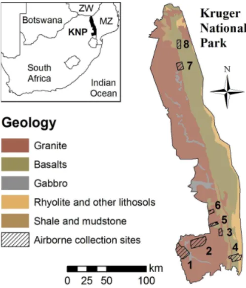
Fig. 1. Study site locations and geology. Numbers correspond to site ID in Table 1. Zw = Zimbabwe, MZ = Mozambique, KNP = Kruger National Park.
landscapes were flown in 2008 covering 70 978 ha of KNP’s major substrate, topographic, and climatic gradients (Fig. 1). KNP is roughly split into equal halves of granite in the west and basalt in the east, with granite substrates weathered to sandy, nutrient-poor soils and basalts weathered to clay-rich, primarily smectitic soils (Venter and Scholes, 2003). The granitic landscapes exhibit distinct catena patterns, despite the shallow nature of the hillslopes (3–5◦). In contrast the southern basalts are flatter (0.5–1◦) and exhibit a linear in-crease in clay content from 30 % to 60 % from crest to toes-lope (Venter and Scholes, 2003). Gabbro intrusions are scat-tered throughout the park and are also weathered to clay-rich, smectitic soils.
The climate of KNP is primarily semi-arid, with mean annual temperature and precipitation (MAP) of 22◦C and 550 mm yr−1, respectively, and an average potential evapora-tion of 7 mm day−1(Du Toit et al., 2003). The precipitation is primarily rainfall, which ranges from∼300–500 mm yr−1 in the north to 500–700 mm yr−1 in the south, and a simi-lar east-west gradient in the south. Granite catena soil depth and seepline distance from crest are known to increase with MAP in KNP (Olbrich, 1984; Chappel, 1993; Khomo, 2008; Levick et al., 2010).
The woody species commonly associated with the south-ern granites (e.g. Skukuza) consist of broadleaf
Combre-tum spp. on crests, little woody cover on the backslope, and
a sparse cover of fineleaf Acacia shrubs and stunted trees on the toeslope. The southern basalts support sparse woody cover of Acacia spp. and large marula (Sclerocarya
bir-rea), although it is largely unknown whether a vegetation
catena pattern similar to that on the granites exists here. The northern Shingwedzi and Roan landscapes are dominated by Colophospermum mopane. Few studies of woody AGB
have previously been conducted in the park, although stud-ies in savannas of similar vegetation and climate estimate KNP woody AGB to range from 10–40 Mg ha−1 (Scholes and Walker, 1993; Du Toit et al., 2003). Most recently Nick-less et al. (2011) estimated AGB at 22.9 Mg ha−1using a 4 ha field plot in KNP on a granite substrate near Skukuza.
Herbivore and fire exclosures, setup and maintained by KNP researchers, were utilized to investigate AGB in the ab-sence of fire and herbivory. The experimental design and his-tory of the exclosures are described by Levick et al. (2009), Trollope et al. (2008), and Asner et al. (2009). The two ex-closures included here are those located within the airborne study landscapes of Pretoriuskop and Lower sabie and had treatment durations of 36 yr and 34 yr, respectively.
2.2 Field biomass estimation
Field inventories were conducted within the extent of the Li-DAR data during the overflights in April–May 2008 to in-form and validate airborne estimates of AGB. Field plots (n=124) of equal size (30 m diameter, 0.07 ha) were es-tablished for LiDAR-biomass calibration. Riparian wood-lands adjacent to major rivers (Strahler stream order ∼5 and greater) were not included in this study as they require a separate calibration and represent less than 2 % of KNP land area. Biomass along smaller streams and drainage lines was included the study. The center of each field plot was recorded using hand-held, differentially corrected GPS re-ceivers (GeoXT Trimble Inc., GS50 Leica Geosystems Inc.) to enable accurate registration of field-estimated AGB to airborne LiDAR data. Within each plot, basal stem diame-ter (10 cm above basal swelling), height, and species were recorded for all woody stems greater than 5 cm diameter and 1.5 m height.
0 1 2 3 4 5 0 5 0 100 150 Combretum spp. F iel d A G B ( M g/ha
) Training stats:m=44.4HCC+ 9.9 R^2 0.74 CV 0.44 RMSE 18.4
0 1 2 3 4 5
0
5
0
100
150
Acacia spp. & marula
Training stats:
m=25.6HCC+6.1 R^2 0.82 CV 0.48 RMSE 11.6
0 1 2 3 4 5
0 5 0 100 150 C.mopane Training stats:
m=29.6HCC+2.1 R^2 0.94 CV 0.3 RMSE 13.1
H(m) x CC(%)
0 50 100 150
0 50 100 150 Combretum spp. F iel d A G B ( M g /h a) 1:1 Cross-validation stats:
CV 0.46 RMSE 19.4
0 50 100 150
0
50
100
150
Acacia spp. & marula
1:1
Cross-validation stats:
CV 0.54 RMSE 13.2
0 50 100 150
0 50 100 150 C.mopane 1:1 Cross-validation stats:
CV 0.39 RMSE 16.8
Predicted AGB (Mg/ha)
a
b
c
e
f
d
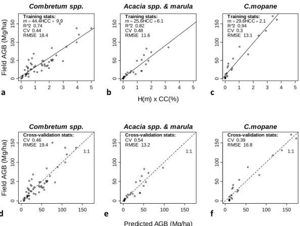
Fig. 2. Model calibration and cross-validation to predict AGB using airborne LiDAR. Points represent calibration field plots. Three models were trained according to dominant woody species: (a) mixed broadleaf (Combretum apiculatum, Combretum collinum) and fineleaf (Acacia
nigrescens, Dichrostachys cinerea) savanna (b) Acacia spp. and marula (Sclerocarya birrea) savanna (c) mopane (Colophospermum mopane)
savanna. (d–f) Observed AGB vs. predicted AGB with test RMSE and coefficient of variation (CV) estimated usingk-fold cross-validation
(k= 3).
2.3 Airborne biomass calibration
In April–May of 2008, the Carnegie Airborne Observatory (CAO) collected over 700 km2 of discrete-return LiDAR data at a pulse repetition frequency of 50 kHz to generate three-dimensional maps of tree canopy structure at 1.12 m laser spot spacing (for the aircraft altitude flown at 2000 m). Flights were planned with 100 % repeat coverage and there-fore LiDAR point density averaged two points per 1.12 m spot. LiDAR spatial errors were less than 0.20 m vertically and 0.36 m horizontally (Asner et al., 2007, 2009). A veg-etation height map, where each 1.12 m pixel represents the canopy height above ground (m), was computed from the LiDAR point cloud by subtracting a ground DEM (classi-fied from LiDAR last return elevation) from a canopy surface DEM (first return elevation). This vegetation height map was then used to calculate the following plot-level LiDAR met-rics. Plot top-of-canopy height,H, is computed as the mean of all 564 pixel height values within each 30 m diameter plot circle centered at each GPS location. A height threshold iden-tical to that used in the field (less than 1.5 m) masked out grass and ground misclassified as vegetation. Plot canopy
cover (CC) is computed as the number of pixels>1.5 m in height divided by 564 (total pixels inside a plot). A total of 124 upland field plots were used to train the LiDAR-biomass regression models.
H×CC was selected as the final LiDAR metric based on best goodness-of-fit, lowest uncertainty, and most parsimo-nious (Fig. 2a–c). TheH×CC metric is also ecologically relevant, as it is roughly proportional to wood volume. The best fit was linear; more complex models were tested, such as log-log and multivariate regressions usingH, CC,H×CC, but none of the more complex models improved goodness-of-fit (R2)or predictive uncertainty (RMSE, CV).
The final regression models (Fig. 2a–c) were trained on data stratified by the three dominant woody species associa-tions found in the park: mixed Combretum spp., marula and
Acacia spp, and mopane. Species with higher wood density
have steeper model slopes, whereas those with large crown areas relative to AGB have shallower model slopes, such as
Sclerocarya birrea and multi-stemmed Combretum apicu-latum. K-fold cross-validation usingk=3 was performed to estimate predictive uncertainty (RMSE) and bias for each model. Maps of AGB were created by applying the regres-sion models (Fig. 2a–c) to LiDAR vegetation height maps. 2.4 Regional analysis and landscape modeling
To study edaphic and hillslope morphological controls over AGB, regional maps of geological and soil classes were ac-quired from the South African National Park Service (Ven-ter and Scholes, 2003). For the hillslope-scale studies, (Ven- ter-rain elevation at 1 m horizontal resolution was acquired from ground digital elevation maps (DEMs) derived from the CAO LiDAR data. A relative elevation map (REM) was computed using the LiDAR DEM as input to the ArcGIS Hydrology Toolbox (ArcMap 9.2 ESRI Inc.), and the difference between the elevation at each pixel and the elevation of the nearest stream is defined here as Elevation Above Stream (EAS). All AGB statistics were performed inR and uncertainty is reported as mean±2 SE (standard error of the mean).
3 Results
3.1 Hillslope and regional variation in biomass
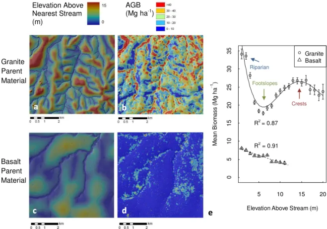
On granitic substrate AGB was highly spatially correlated with hillslope position. Of the topo-edaphic variables tested, EAS was the most strongly correlated with AGB. At the orig-inal scale of AGB prediction (0.07 ha), slope, profile con-vexity, and other morphologic variables were poorly corre-lated with AGB, yet they were increasingly correcorre-lated at the larger spatial scale used for subsequent landscape model-ing (0.5 ha). LiDAR estimates of ground elevation and slope found the granitic hillslopes to be shallow to moderately un-dulating (0.6–4.8◦slope, 95 % CI of natural landscape vari-ance), with even shallower gradients on the basalts (0.5–2.1◦ slope, 95 % CI). Figure 3 illustrates the strong correlation of EAS to AGB on the Skukuza granite landscape. Here a clear, nonlinear AGB pattern emerged as a function of EAS, with high AGB along stream corridors (34.1±1.4 Mg ha−1
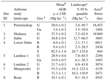
Table 1. Airborne-estimated mean biomass and landscape variation in AGB (0.5 ha per sample).
Meanb Landscapec Airborne AGB 5–95 % Aread Site study µ±2 SE quantile flown ID landscape Geoa (Mg ha−1) (Mg ha−1) (ha)
1 Pretoriuskop G 20.0±0.2 2.6–49.7 18,453 Ga 3.4±0.2 1.5–10.0 1404 2 Skukuza G 27.5±0.2 7.2–63.9 18 860 3 Sabie G 36.8±0.4 12.7–66.5 3603 4 Lower Sabie B 6.0±0.1 2.1–17.1 6011 R 9.4±0.3 2.3–28.5 2436 S 82.5±1.6 26.7–135.6 844 5 Landuse 1 G 28.9±0.6 7.0–65.5 2296 Ga 15.0±0.5 6.1–36.3 1093 6 Landuse 2 G 21.7±0.3 6.8–43.8 3074 7 Shingwedzi G 53.3±0.8 14.3–122.4 4139 B 31.3±1.1 10.2–110.9 2671 8 Roan B 10.1±0.1 8.1–16.3 4543
aGeology: G = granite, Ga = gabbro, B = basalt, S = shale, R = rhyolite. bMean AGB±2×standard error of the mean.
cLandscape-scale AGB variance expressed as 5 % to 95 % quantiles. dArea flown. Note the number of AGB samples = 2×area flown
(each AGB pixel is 0.5 ha).
(2×SE) at 0–1 m above nearest stream), then declining to 17.7±0.5 Mg ha−1on footslopes before increasing again to 26.8±0.8 Mg ha−1on crests. A fourth-order polynomial was the most parsimonious model fit to mean AGB and achieved a coefficient of determination ofR2= 0.87 using EAS as the sole independent variable. A model of this same form was also tested on the raw AGB estimates (not means), but it ac-counted for less variance in AGB (R2= 0.11) due to high AGB variability at the plot scale (27 m) from other factors (e.g. fire history, herbivory, stream order), uncertainty in the LiDAR-AGB calibration, and natural variance in peak crest heights.
The above analysis was also conducted on basalt near Lower Sabie (Fig. 3d). AGB followed a linear decline from 8.1±0.2 Mg ha−1 near streams down to 4.1±0.2 Mg ha−1 at the crest. Higher order functions of EAS did not improve goodness-of-fit nor reduce AGB standard error. Basalt mean AGB was 6.5±0.06 Mg ha−1, nearly a factor of four lower than on the granites. The linear model using relative eleva-tion alone accounted for 91 % of the variance in mean AGB at the hillslope scale, yet, as on the granites, relative eleva-tion accounted for much less AGB variance at the plot-scale (R2= 0.0018).
5 10 15 20
0
5
10
15
20
25
30
35
Elevation Above Stream (m)
M
e
a
n
B
io
m
a
ss
(M
g
h
a
1 )
Granite Basalt
Riparian
Footslopes
Granite Parent Material
Crests
a
b
R2 = 0.87
R2 = 0.91
Basalt Parent Material
d
c
e
a
b
c
d
Elevation Above Nearest Stream (m)
AGB (Mg ha-1)
Fig. 3. Spatially explicit correlation of elevation above nearest stream (a, c)) to LiDAR-estimated AGB (b, d)) for granite (Skukuza, top row) and basalt (Lower Sabie, bottom row). Each point in the graph (e) represents the mean of all biomass pixel values (0.07 ha resolution)
within a one meter bin of elevation for the extents shown in (b, d). Error bars are 2×standard error of the mean. Note increase in AGB
on granitic crests above the seepline (∼7 m), whereas mean AGB on basalts exhibits a linear decrease in AGB for all elevation gain above
nearest stream. Solid curve is the granite, best-fit polynomial model of (fourth order) withR2= 0.87 and dashed line is the substrate best-fit model (R2= 0.91). Note the basalt error bars are drawn but are smaller than the point icons.
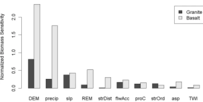
3.2 Biomass sensitivity analysis
To assess the relative influence of topographic and edaphic variables on AGB, landscape models were developed to en-able a biomass sensitivity analysis. The landscape models were created using LiDAR-derived AGB as the response variable and the following predictor variables: ground eleva-tion above sea level, slope, profile convexity, plan convexity, aspect, topographic wetness index (TWI), elevation above nearest stream (REM), distance to nearest stream, Strahler stream order, and flow accumulation. A simple one-at-a-time (OAT) screening (Fig. 5) was conducted to observe the first-order sensitivity of AGB to these factors. Absolute elevation had the highest AGB sensitivity on both granite and basalt substrates, followed by slope and relative elevation. Strong linear sensitivity to relative elevation on basalt and weak lin-ear sensitivity on granite are to be expected, given the pat-terns observed at the hillslope scale in Fig. 3. Consequently, stream distance also had high AGB sensitivity on the grad-ual basaltic slopes, where stream distance strongly co-varies with EAS and slope.
AGB sensitivity continued to decrease with flow accumu-lation, profile convexity, and stream order. However, AGB sensitivity to stream order was underestimated because the highest order streams (5–6) were excluded by the 95 % CI range selection and AGB varies nonlinearly with stream or-der. Aspect, topographic wetness index, and flow accumu-lation had low biomass sensitivity and were excluded from the final model. Several factors with low sensitivity in the OAT analysis were included in the final model due to non-linear effects that, when modeled below, increase the factor’s AGB sensitivity (such as with relative elevation on gran-ite). Figure 5 shows the KNP biomass map resulting from applying the final landscape models across the entirety of the park, allowing visualization of how topo-edaphic factors influence AGB.
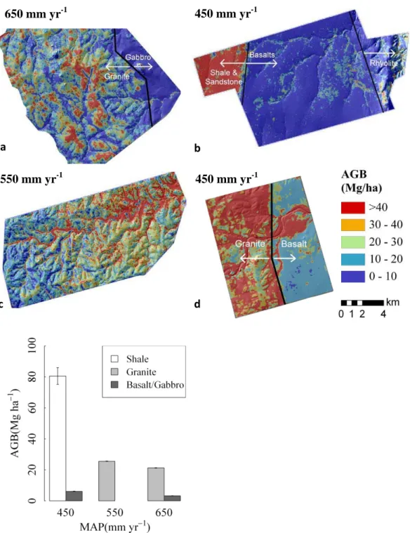
650 mm yr
-1450 mm yr
-1e
c
d
550 mm yr
-1450 mm yr
-1a
b
Fig. 4. LiDAR-derived AGB overlaying topographic hillshade for reference for four landscapes: (a) Pretoriuskop (b) Lower Sabie (c) Skukuza (d) Shingwedzi (e) Mean landscape AGB (±2 SE) across substrate and precipitation gradients, controlling for radiation, temperature, and species composition (excludes Shingwedzi due to different radiation and vegetation physiognomy).
was selected if it considerably reduced residual error and im-proved goodness-of-fit to the raw data. EAS and distance to stream had third degree effects on AGB, similar in shape to those observed at the hillslope scale (Fig. 3). Stream order was quadratic due to rapidly increasing AGB along higher order streams. Precipitation was also best modeled using a quadratic term to capture low AGB at MAP extremes (450
Fig. 5. Biomass sensitivity to landscape factors: a simple one-at-a-time (OAT) screening to observe the first-order, additive response of AGB to an initial set of landscape factors. Factors shown are DEM = ground elevetation above sea level, precip = precipitation, slp = slope, REM = Relative Elevation Model (height above near-est stream), strDist = distance to nearnear-est stream, flwAcc = stream flow accumulation, proC = profile convexity, strOrder = stream Or-der, asp = aspect, TWI = topographic wetness index.
(fromR2= 0.10 to R2= 0.15 at the 0.5 ha scale). Table C1 (Appendix C) lists these models for each substrate type. 3.3 Park-wide biomass
In order to provide a baseline for park management to de-tect future change in AGB (e.g. due to woody encroachment, mega-herbivore impacts, etc.), we estimated total woody AGB in KNP to be 53.8 Gg dry matter, or equivalently a park-wide mean AGB density of 28.3 Mg ha−1. This estimate ex-cludes woodlands along riparian corridors, which account for
∼2–4 % of the park’s area. Park-wide total biomass was esti-mated by multiplying the land area of each land system from Venter and Scholes (2003) by our corresponding mean land-scape AGB estimated from LiDAR (Table 1). Dividing by the area of KNP (∼1.9 Mha) yields park-wide mean AGB.
4 Discussion
4.1 Hillslope geomorphologic controls over biomass
The gradual nature of basalt slopes (<1◦mean terrain gradi-ent), typically hundreds of meters if not kilometers in length, along with generally sparse woody cover (∼5 %), make it difficult in the field to quantify spatial variation in AGB on basalts. Yet with LiDAR measurements, we observe double the AGB on toeslopes relative to crests on basalts (Fig. 3e), with a strong, linear negative relationship between AGB and hillslope position. This AGB gradient is likely the result of high A horizon clay content (30–60 %) along the entirety of the slope (Venter and Scholes, 2003), leading to predomi-nantly overland flow and accumulation of water downslope, as well as potentially shallower soils on basaltic crests. This stands in contrast to the coarse-sandy granite A horizons, which permit higher infiltration rates and subsoil
through-flow on crests. Although a concomitant CEC increase with clay content from basalt crest to toeslope was observed by Venter and Scholes (2003), phosphorous and micronutrient concentrations (K, Ca, Mg) were relatively constant (N con-tent not available), indicating soil nutrients do not follow the same catena pattern observed in clay content and AGB.
Although the linear relationship between hillslope position and AGB on basalts can be interpreted as a catena pattern, it differs in shape and magnitude relative to the granite cate-nas. Apart from an overall higher mean AGB on granites, the primary distinction in granite catena shape is a dip in AGB on footslopes, with 50 % higher AGB on crests and 90 % higher along streams (Fig. 3e). The mean seepline location of 7 m EAS identified by Levick et al. (2010) in the Skukuza granitic landscape coincides with our lowest mean AGB (17.7±0.5 Mg ha−1) (Fig. 3e). The soil properties downs-lope of the seepline, namely B horizons with 20–30 % clay and hardpan commonly near the surface of these Solonzetic soils, likely account for the lower AGB on footslopes rela-tive to crests. Termite bioturbation of sandy crest soils may also increase hydraulic conductivity and concentration of soil nutrients, thereby accentuating the difference between crest and footslope AGB (Scholes and Archer, 1997). Recent work has found that termite mounds are primarily found on sandy crests, with the lower extent of mounds coinciding with the seepline (Levick et al., 2010).
4.2 Regional controls over biomass
At the regional scale precipitation sets an upper bound for potential woody cover in African semi-arid savannas, with soil and disturbance regimes determining the extent to which this potential is realized (Sankaran et al., 2005). In KNP east-west and north-south rainfall gradients have been hy-pothesized to be largely responsible for regional variation in woody cover (Du Toit et al., 2003). Yet here we observed sev-eral sharp transitions in AGB which follow geologic bound-aries (Fig. 4) that occur over short distances (<1 km) where there is negligible variation in MAP, allowing us to control for rainfall while comparing AGB between substrate types. Multiple study landscapes spanning the KNP rainfall gradi-ent permit a factorial analysis of rainfall and substrate effects on AGB.
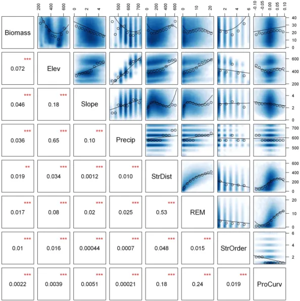
Fig. 6. Interactions between biomass and landscape factors. Top row indicates correlation of LiDAR-derived AGB to landscape variables for
n= 82 503 CAO biomass pixels (0.5 ha/pixel) on southern granite substrate. All other rows indicate interactions between landscape factors.
Blue intensity indicates point density of the raw data. Curves are the most parsimonious models fit to the raw data. Circles are median
values sampled at set intervals to visualize underlying patterns in the raw data (blue). Numbers in lower-left half areR2for the model curve
shown in the corresponding scatter plot, and stars indicate statistical significance (**p <0.01, ***p <0.001) but not necessarily ecological
relevance. Landscape factors shown are: elevation above sea level (m), slope (deg), precipitation (mm yr−1), distance from nearest stream
(m), relative elevation model (height above nearest stream) (m), stream order, and profile curvature (positive values are convex) (deg/m).
second landscape at low precipitation is Shingwedzi in north-ern KNP (Fig. 4), where we find the same relative differ-ence in AGB between granite and basalt (3–4 times higher on granites) as that found in southern KNP.
On the high end of the precipitation gradient (650 mm yr−1), mean AGB on Pretoriuskop granites is 27 % lower than on Skukuza granites, which is consistent with other studies attributing this westward decrease in woody cover to higher precipitation, grass biomass, and fire intensity (Trollope and Potgieter, 1986; Du Toit et al., 2003). However, the Pretoriuskop CAO data also reveal the discon-tinuity in AGB between the primary granite substrate and a
4.3 Topo-edaphic controls in the context of fire and herbivory
Several hypotheses suggest the basalt-derived soils are a proximal constraint on woody vegetation, including high clay content in the A horizon preventing adequate infil-tration, shrinking/swelling of smectitic clays tearing roots, or higher nutrient concentrations allowing grasses to out-compete woody plants more than on granites (Scholes and Archer, 1997; Venter and Scholes, 2003). However, the idea that any of these effects are a proximal limitation to woody plant AGB is contradicted by our results from the Makhohlola experimental herbivore and fire exclosure, lo-cated in a KNP basalt landscape (Trollope et al., 2008; Lev-ick et al., 2009). Mean AGB is more than ten-fold higher in-side the exclosure (36.9±7.1 Mg ha−1vs. 2.7±0.5 Mg ha−1 in and out, respectively). Higher AGB inside the exclosure demonstrates that these basalt-derived soils are capable of supporting AGB higher than what is observed on granites, in the absence of fire and herbivory (consistent with higher phosphorus and micronutrient availability). Another exclo-sure of similar age on a granite substrate with lower herbivore carrying capacity and slightly lower fire intensity near Pre-toriuskop (Trollope et al., 2008) showed no significant dif-ference in AGB inside and outside the exclosure (P =0.45, n=500, 22.0±1.2 Mg ha−1inside and 22.7±1.3 Mg ha−1 outside), suggesting AGB on granite substrates is less af-fected by fire and herbivory. While a detailed analysis of AGB effects from excluding herbivory and fire is outside the scope of this study, these results demonstrate fire-herbivore interactions play a critical role in down-regulating AGB on basalts, and that edaphic mechanisms alone cannot account for lower AGB on basaltic landscapes.
5 Summary
In savanna ecosystems with heterogeneity at multiple spa-tial scales, airborne LiDAR provides the large-area measure-ments needed to reveal woody vegetation patterns otherwise obscured by local variance in AGB. We found the relation-ship between biomass and hillslope position differ both in shape and direction between parent materials, with a negative linear trend on basalts (low AGB on crests increasing downs-lope), in contrast to the predicted pattern found on granites, with high AGB on crests, low AGB on backslopes, and high AGB near streams. We hypothesize subsoil throughflow ac-counts for higher AGB on granitic crests, whereas overland flow dominates basalt landscapes, allowing water accumula-tion downslope to subsidize woody plant growth hindered by frequent grass fires and large ungulate populations.
At regional scales climate sets an upper bound on AGB, yet we found AGB is more sensitive to parent material than to precipitation within Kruger’s semi-arid MAP gradient (400– 800 mm−1yr), with large differences in mean AGB occurring
over short distances that coincide with geologic boundaries. By mapping AGB within and outside fire and herbivore ex-closures, we found that basalt-derived soils can support ten-fold higher AGB in the absence of fire and herbivory, sug-gesting high clay content alone is not a proximal limitation on AGB. Understanding how fire and herbivory contribute to AGB heterogeneity is critical to predicting future savanna carbon storage under a changing climate, as well as under-standing how fuelwood resources are limited or enhanced by the landscape.
Appendix A
Stem allometry methods
Stem biomass was estimated from field-measured stem diam-eter using the following broad-leafed generalized equation from Nickless et al. (2011):
AGB=e−3.47Ds2.83×e0.212
(Nickless et al., 2011) (A1)
where AGB is aboveground woody plant dry mass (kg) and Ds is basal stem diameter (cm). This regression (R2= 0.98, n= 443, MSE = 0.12 (ln(kg))2) was calibrated using broadleaf species commonly found in southern KNP: Combretum apiculatum, Sclerocarya birrea,
Termina-lia sericea, Spirostachys africana, Euclea divinorum, and
other broad-leafed species (Nickless et al., 2011). For multi-stemmed trees, biomass was calculated separately for each stem’s diameter and then summed. Solving for AGB by tak-ing the natural exponential of the original log-log regres-sion derived by Nickless et al. (2011) results in an under-prediction of stem biomass because least-squares regression assumes the response variable (AGB) is normally distributed, when in fact it is log-normally distributed (Beauchamp and Olson, 1973). To account for this we multiply by the correc-tion factor CF =eσ
2
2 to arrive at Eq. (1), whereσ2is the mean square error (MSE) in log form from Nickless et al. (2011).
Appendix B
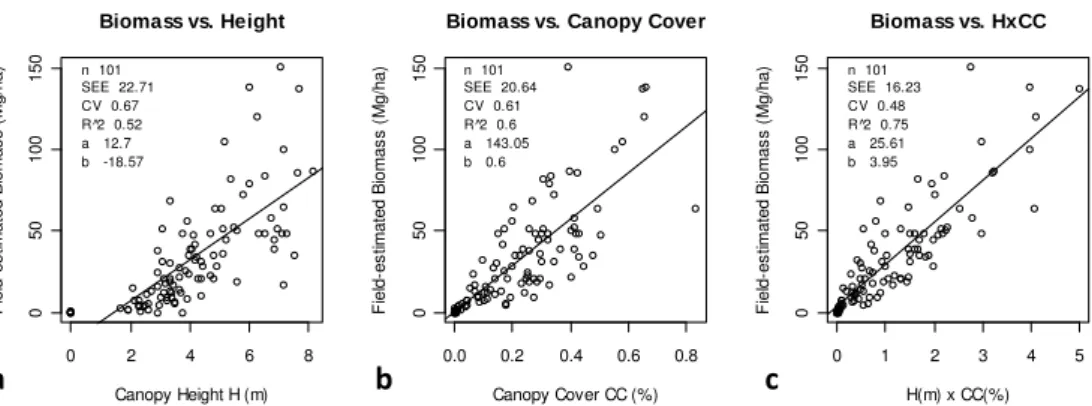
LiDAR-biomass calibration curves using only height or canopy cover
0 2 4 6 8
0
50
10
0
150
Biomass vs. Height
Canopy Height H (m)
F iel d-es tim at e d B iomas s ( M g/ h
a) n 101
SEE 22.71 CV 0.67 R^2 0.52 a 12.7 b -18.57
0.0 0.2 0.4 0.6 0.8
0
50
10
0
150
Biomass vs. Canopy Cover
Canopy Cover CC (%)
F iel d-es tim at e d B iomas s ( M g/ h
a) n 101
SEE 20.64 CV 0.61 R^2 0.6 a 143.05 b 0.6
0 1 2 3 4 5
0
50
10
0
150
Biomass vs. HxCC
H(m) x CC(%)
F iel d-es tim at e d B iomas s ( M g/ h
a) n 101
SEE 16.23 CV 0.48 R^2 0.75 a 25.61 b 3.95
b
c
a
Fig. B1. Comparison of biomass calibration curves using height (H), canopy cover (CC), andH×CC as predictor variables. All 101 field plots from southern KNP across a range of dominant woody species were used to compare these three predictors. An additional 23 plots from northern KNP are dominated by C.mopane with significantly different morphology and stand densities than southern KNP, and thus received
a separate calibration curve (Fig. 2c). Log-log and multivariate regressions usingH, CC,H×CC were also tested, but none improved
good-ness-of-fit (R2)or predictive performance (SEE, CV) compared to these linear fits.
Appendix C
Landscape modeling results
Table C1. Landscape models describing the relation of AGB to seven landscape factors at 0.5 ha resolution. Area = the fraction of KNP
cov-ered by each model type,µ= mean ofnCAO AGB estimates at 0.5 ha/pixel, all other columns are model results. Polynomial terms up to
4th-order were tested for each factor to maximize goodness-of-fit while minimizing the number of terms and the standard error. Shale is a cons-tant because only a small area of homogenous vegetation structure (A.harveyi thickets) was flown by CAO, insufficient in size for land-scape modeling.
Model Type Area % µ±2 SE (Mg ha−1)
RMSE
(Mg ha−1) CV Adj-R
2
n(pixels) Landscape Model Formulaa
1. Granite –
Comb/ Acacia
30 % 24.7±0.06 16.7 0.68 0.148 82 503
B= 143.6−0.5654r+ 0.08934r2− 0.002818r3−0.3387d+ 0.0003409d2− 2.549s+ 33.65c−0.1222p+ 0.0001157p2− 0.003492t−2.235m+ 0.6113m2
2. Basalt –
Acacia 19 % 6.5± 0.06 6.3 0.97 0.149 15 243
B=−24.09 + 0.3967r+ 0.2014d− 0.0003d2+ 1.278s−0.00645t
3. Granite –
C.mopane 25 % 51.6± 0.44 35.8 0.69 0.118 7453
B= 835.9 + 3.730r−0.5329R2+ 0.01467r3− 11.86d+ 0.01802d2+ 3.547s+ 160.3c+ 5.429p−0.006301p2−0.04384t− 0.3154m+ 1.499m2
4. Basalt –
C.mopane 16 % 17.9±0.24 22.9 1.28 0.327 13 370
B=−19.33−11.54r+ 11.66R2−1.527r3−
0.1345d+ 7.348s+ 0.2078p− 15.33m+ 3.33m2
5. Rhyolite 7 % 8.8±0.14 7.9 0.89 0.253 4282
B= 18.19−0.8432r+ 0.06936R2− 0.001499r3−0.02544d+ 1.822s− 27.37c−0.02435p−0.008515t+ 2.470m− 0.3632m2
6. Shale 4 % 82.1±0.86 31.5 0.38 0.145 1557 B= 82.1
TOTAL
(park mean) 100 % 28.3±0.06 – – – –
aMultivariate, non-linear models for predicting AGB using landscape-only variables at 0.5 ha scale. Variable legend:B= aboveground wood biomass (Mg ha−1),r= elevation
above nearest stream (m),d= elevation above sea level (m),s= slope (deg),c= profile curvature (deg m−1),p= precipitation (mm yr−1),t= stream distance (m), and
specific gravity and form factors: AGBjenkins=e−2.01DBH2.43×e
(0.236)2 2
(Jenkins et al., 2003) (A2)
where DBH is diameter (cm) at breast height (n= 485, dmax= 230 cm).
For the northern landscapes dominated by
Colophosper-mum mopane shrub savanna, the species-specific
equa-tion substantially improved AGB to airborne-LiDAR metrics (Fig. 2f) and was used in place of Eq. (1) for stems of this species (also with correction factor):
AGBmopane=e−2.77DBH2.49×e (0.263)2
2
(Nickless et al., 2011) (A3)
Acknowledgements. We thank I. Smit, D. Pienaar, and the entire
SANParks staff for their outstanding logistical and scientific sup-port. This research was funded by a grant from the Andrew Mellon Foundation. The Carnegie Airborne Observatory is supported by the W. M. Keck Foundation, the Gordon and Betty Moore Foundation, the Grantham Foundation for the Protection of the Environment, and William Hearst III.
Edited by: R. Conant
References
Alizai, H. U. and Hulbert, L. C.: Effects of soil texture on evapora-tive loss and available water in semi-arid climates, Soil Sci., 110, 328, doi:10.1097/00010694-197011000-00006, 1970.
Archer, S.: Tree-grass dynamics in a prosopis-thornscrub savanna parkland – reconstructing the past and predicting the future,
´
Ecoscience, 83, 2, 83–99, ISSN: 11956860, 1995.
Asner, G. P.: Tropical forest carbon assessment: integrating satel-lite and airborne mapping approaches, Environ. Res. Lett., 4, 034009, doi:10.1088/1748-9326/4/3/034009, 2009.
Asner, G. P., Knapp, D. E., Kennedy-Bowdoin, T., Jones, M. O., Martin, R. E., Boardman, J., and Field, C. B.: Carnegie airborne observatory: in-flight fusion of hyperspectral imaging and waveform light detection and ranging for three-dimensional studies of ecosystems, J. Appl. Remote Sens., 1, 013536, doi:10.1117/1.2794018, 2007.
Asner, G. P., Levick, S. R., Kennedy-Bowdoin, T., Knapp, D. E., Emerson, R., Jacobson, J., Colgan, M. S., and Martin, R. E.: Large-scale impacts of herbivores on the structural di-versity of African savannas, P. Natl. Acad. Sci., 106, 4947, doi:10.1088/1748-9326/4/3/034009, 2009.
Beauchamp, J. J. and Olson, J. S.: Corrections for bias in regression estimates after logarithmic transformation, Ecology, 54, 1403– 1407, 1973.
Belsky, A. J.: Influences of trees on savanna productivity: tests of shade, nutrients, and tree-grass competition, Ecology, 75, 922– 932, 1994.
Bern, C., Chadwick, O., Hartshorn, A., Khomo, L., and Chorover, J.: A mass balance model to separate and quantify colloidal and solute redistributions in soil, Chem. Geol., 282, 113–119, 2011.
Bond, W. J. and Keeley, J. E.: Fire as a global “herbivore”: the ecology and evolution of flammable ecosystems, Trends in Ecol. Evol., 20, 387–394, 2005.
Brady, N. C. and Weil, R. R.: The nature and properties of soils, 11 Edn., Prentice-Hall Inc., 1996.
Chappel, C.: The Ecology of Sodic Sites in the Eastern Transvaal Lowveld, Unpublished M.Sc. thesis, University of Witswater-srand, Johannesburg, South Africa, 1993.
Coughenour, M. B. and Ellis, J. E.: Landscape and climatic control of woody vegetation in a dry tropical ecosystem: Turkana Dis-trict, Kenya, J. Biogeogr., 20, 383–398, 1993.
Drake, J. B., Dubayah, R. O., Clark, D. B., Knox, R. G., Blair, J. B., Hofton, M. A., Chazdon, R. L., Weishampel, J. F., and Prince, S.: Estimation of tropical forest structural characteristics using large-footprint lidar, Remote Sens. Environ., 79, 305–319, 2002. Du Toit, J. T., Rogers, K. H., and Biggs, H. C.: The Kruger
Experi-ence, Island Press, 2003.
Eckhardt, H., Wilgen, B., and Biggs, H.: Trends in woody vegeta-tion cover in the Kruger Navegeta-tional Park, South Africa, between 1940 and 1998, Afr. J. Ecol., 38, 108–115, doi:10.1046/j.1365-2028.2000.00217.x, 2000.
Fensham, R. J. and Fairfax, R. J.: Drought-related death of savanna eucalypts: species susceptibility, soil conditions and root archi-tecture, J. Veg. Sci., 18, 71–80, 2007.
Jenkins, J. C., Chojnacky, D. C., Heath, L. S., and Birdsey, R. A.: National-scale biomass estimators for United States tree species, Forest Sci., 49, 12–35, 2003.
Khomo, L.: Weathering and soil properties on old granitic cate-nas along climo-topographic gradients in Kruger National Park, 2008.
Khomo, L., Hartshorn, A. S., Rogers, K. H., and Chadwick, O. A.: Impact of rainfall and topography on the distribution of clays and major cations in granitic catenas of southern Africa, Catena, 2011.
Lefsky, M. A., Harding, D., Cohen, W., Parker, G., and Shugart, H.: Surface lidar remote sensing of basal area and biomass in decid-uous forests of eastern Maryland, USA, Remote Sens. Environ., 67, 83–98, 1999.
Levick, S. R. and Rogers, K.: Context-dependent vegetation dy-namics in an African savanna, Landscape Ecol., 26, 515–528, doi:10.1007/s10980-011-9578-2, 2011.
Levick, S. R., Asner, G. P., Kennedy-Bowdoin, T., and Knapp, D. E.: The relative influence of fire and herbivory on savanna three-dimensional vegetation structure, Biol. Conserv., 142, 1693– 1700, 2009.
Levick, S. R., Asner, G. P., Chadwick, O. A., Khomo, L. M., Rogers, K. H., Hartshorn, A. S., Kennedy-Bowdoin, T., and Knapp, D. E.: Regional insight into savanna hydrogeomorphology from termite mounds, Nature Communications, 1, 1–7, 2010.
Milne, G.: Normal erosion as a factor in soil profile development, Nature, 138, 548–549, 1936.
Morrison, C.: The catena and its application to tropical soils, Com-monwealth Bureau of Soil Science Technical Bulletin, 46, 124– 130, 1948.
Munnik, M., Verster, E., and Rooyen, T.: Spatial pattern and vari-ability of soil and hillslope properties in a granitic landscape 1. Pretoriuskop area, S. Afr. J. Plant Soil, 7, 121–130, 1990. Nickless, A., Scholes, R., and Archibald, S.: A method for
calcu-lating the variance and confidence intervals for tree biomass es-timates obtained from allometric equations, Afr. J. Sci.,107(5/6), 356, doi:10.4102/sajs.v107i5/6.356, 2011.
Olbrich, B.: A study on the determinants on seepline grassland width in the Eastern Transvaal lowveld, Unpublished B.Sc. hon-ors project, University of Witwatersrand, Johannesburg, South Africa, 1984.
Ruhe, R. V.: Elements of the soil landscape, 165–170, 1960. Sankaran, M., Ratnam, J., and Hanan, N. P.: Tree–grass coexistence
in savannas revisited-insights from an examination of assump-tions and mechanisms invoked in existing models, Ecol. Lett., 7, 480–490, 2004.
Sankaran, M., Hanan, N. P., Scholes, R. J., Ratnam, J., Augustine, D. J., Cade, B. S., Gignoux, J., Higgins, S. I., Le Roux, X., and Ludwig, F.: Determinants of woody cover in African savannas, Nature, 438, 846–849, 2005.
Scholes, R. and Archer, S.: Tree-grass interactions in savannas, Annu. Rev. Ecol. Syst., 28, 517–544, 1997.
Scholes, R. and Walker, B. H.: An African savanna: synthesis of the Nylsvley study, 1993.
Skarpe, C.: Dynamics of savanna ecosystems, J. Veget. Sci., 3, 293– 300, doi:10.2307/3235754, 1992.
Trollope, W. and Potgieter, A.: Estimating grass fuel loads with a disc pasture meter in the Kruger National Park, Journal of the Grassland Society of Southern Africa, 4, 148–152, 1986. Trollope, W., Trollope, L., Biggs, H., Pienaar, D., and Potgieter,
A.: Long-term changes in the woody vegetation of the Kruger National Park, Koedoe-African Protected Area Conservation and Science, 41, 103–112, 2008.
Van Langevelde, F., Van De Vijver, C. A. D. M., Kumar, L., Van De Koppel, J., De Ridder, N., Van Andel, J., Skidmore, A. K., Hearne, J. W., Stroosnijder, L., and Bond, W. J.: Effects of fire and herbivory on the stability of savanna ecosystems, Ecology, 84, 337–350, 2003.
Venter, F. J. and Scholes, R. J.: The Abiotic Template and Its Asso-ciated Vegetation Pattem, The Kruger experience: Ecology and management of savanna heterogeneity, 83, 2003.
Walter, H.: Natural savannahs as a transition to the arid zone, Ecol-ogy of tropical and subtropical vegetation, Oliver and Boyd, Ed-inburgh, 238–265, 1971.
Wiegand, K., Saltz, D., and Ward, D.: A patch-dynamics approach to savanna dynamics and woody plant encroachment-Insights from an arid savanna, Perspectives in Plant Ecology, Evolution and Systematics, 7, 229–242, 2006.