Dimensionality Reduction for Optimal Clustering In Data Mining

(1)

Dimensionality Reduction for Optimal

Clustering In Data

Mining

Ch. Raja Ramesh*, DVManjula, Dr. G. Jena, Dr C V Sastry

*Research Scholar, KL University, Associate Professor Regency Institute of Technology, Yanam. Ch_rajaramesh@yahoo.com,

Associate Professor, KIET, Kakinada, dvmanjula@gmail.com

Professor, B V C College of Engineering, Odalarevu, Amalapuram Professor, SNIT, Hyderabad,cvsastry40@gmail.com

Abstract: Spectral clustering and Leader’s algorithm have both been used to identify clusters that are non-linearly separable in input space. Despite significant research, these methods have remained only loosely related. Sigmoid kernel and polynomial kernel were quite popular for support vector machines due to its origin from clustering. In this paper we are submitting the comparison of above kernel methods after reducing the dimensions using feature functions. For this we have given hand writing data -sets to create and compare the clusters.

Keywords:Sigmoid, polynomial, kernels, Support Vector Machine and leader’s algorithm.

1. INTRODUCTION

Clustering has received a significant amount of attention in the last few years as one of the fundamental problems in data mining. k -means and Leaders’ are most popular clustering algorithms. Recent research has generalized the algorithm in many ways; for example, similar algorithms for clustering can be obtained using arbitrary Bergman divergences as the distortion measure [3]. Other advances include using local search to improve the clustering results [6] and using the triangle inequality to speed up the computation [5].

A major drawback to k -means algorithm is that it cannot separate clusters that are non-linearly separable in input space. Two recent approaches have emerged for tackling such a problem. One is kernel k -means, where, before clustering, points are mapped to a higher-dimensional feature space using a nonlinear function, and then kernel k -means partitions the points by linear separators in the new space. The other approach is

2. PRINCIPAL COPONENT ANALYSIS

Principal component analysis [12] is appropriate when you have obtained measures on a number of observed variables and wish to develop a smaller number of artificial variables (called principal components) that will account for most of the variance in the observed variables. The principal components may then be used as predictor or criterion variables in subsequent analyses. Principal component analysis (PCA) involves a mathematical procedure that transforms a number of possibly correlated variables into a smaller number of uncorrelated variables called principal components. The first principal component accounts for as much of the variability in the data as possible, and each succeeding component accounts for as much of the remaining variability as discrete KarhuncenLoeve transform (KLT), the Hostelling transform or proper orthogonal decomposition (POD). PCA involves the calculation of the eigenvalue decomposition of a data covariance matrix or singular value decomposition of a data matrix, usually after mean centering the data for each attribute. The results of a PCA are usually discussed in terms of component scores and loadings.

PCA is the simplest of the true eigenvectors-based multivariate analysis. Often, its operation can be tough as well as revealing the internal structure of the data in a way which best explains the variance in the data. If a multivariate dataset is visualized as a set of coordinates in a higher-dimensional data space (1 axis per variable) PCA supplies the user with a lower dimensional picture, a “shadow” of this object when viewed from its (in some sense) most of informative viewpoint. PCA is closely related to factor analysis; indeed, some statistical packages deliberately combine the two techniques. True factor analysis makes different assumptions about the underlying structure and solves eigenvectors of a slightly different matrix.

Ch. Raja Ramesh et al. / International Journal on Computer Science and Engineering (IJCSE)

(2)

3. KERNELS

The use of a kernel function is an attractive computational short cut. If we wish to use this approach, there appears to be a need to first create a complicated feature space, and then work out what the inner product in that space would be, and finally find a direct method of computing that value in terms of the original inputs. In practice the approach taken is to define a kernel function directly, hence implicitly defining the feature space. Let us denote clusters by j, and a partitioning of points as { j}kj=1. Using this non-linear function φ,

the objective function of weighted kernel k-means is defined as [1]:

Where (1) Note that mj is the “best” cluster representative since

(2)

The Euclidean distance from to center is given by

= +

- (3)

The dot products φ(a) . φ(b) form the elements of the kernel matrix , K, and can be directly used to calculate distances between points and centroids. All computations are in the form of such inner products, and hence we can replace all inner products by entries of the kernel matrix.

In this way, we avoid the feature space not only in the computation of inner products, but also in the design of the learning machine itself. We will argue that defining a kernel function for an input space is frequently more natural than creating a complicated feature space. Before we can follow this route, however, we must first determine what properties of a function K(x, z) are necessary to ensure that it is a kernel function for some feature space. Clearly the function must be symmetric

K(x,z)={φ(x).φ(z)}={φ(z).φ(x)}=K(z,x) (4)

and satisfy the inequalities that follow from the Cauchy Schwarz inequality, K(x,z)2=(φ(x).φ(z))2≤||φ(z)||2.||φ(x)||2

=(φ(x).φ(x))(φ(x).φ(x))=K(x,x)K(z,z) (5)

These conditions are, however, not sufficient to guarantee the existence of a feature space.

4. Learning Feature Space

The complexity of the target function to be learned depends on the way it is represented and the difficulty of the learning task can vary accordingly. Ideally a representation that matches the specific learning problem should be chosen. So one common preprocessing strategy in machine learning involves changing the representation of the data:

X = (x1 ………xn) φ(x) = (φ1(x) ,. . . . .. ., φn(x)) (6) For eample

G(x,y,z) = ln f(m1,m2,r) = ln C + ln m1 +ln m2 – 2lnr = c+ x+y-2z (7)

(3)

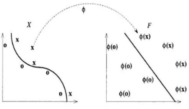
Figure 1 : feature space representation

could be learned by a linear machine.

The fact that simply mapping the data into another space can greatly simplify the task has been known for a long time in machine learning, and has given rise to a number of techniques for selecting the best representation of data. The quantities introduced to describe the data are usually called features, while the original quantities are sometimes called attributes. The task of choosing the most suitable representation is known as feature selection. The space X is referred to as the input space, while is referred as feature space.

The following figure shows an example of a feature mapping from a two dimensional input space to a two dimensional feature space, where the data cannot be separated by a linear function in the input space, but can be in the feature space. The aim of this is to show how such mappings can be made into higher dimensional space where linear separation becomes much easier.

Different approaches to feature selection exist. Frequently one seeks to identify the smallest set of features that conveys the essential information contained in the original attributes. This is known as dimensionality reduction.

X = (x1 ………xn) φ(x) = (φ1(x) ,. . . . .. ., φD(x) ), d < n - (8) 6. EXPERIMENTAL RESULTS

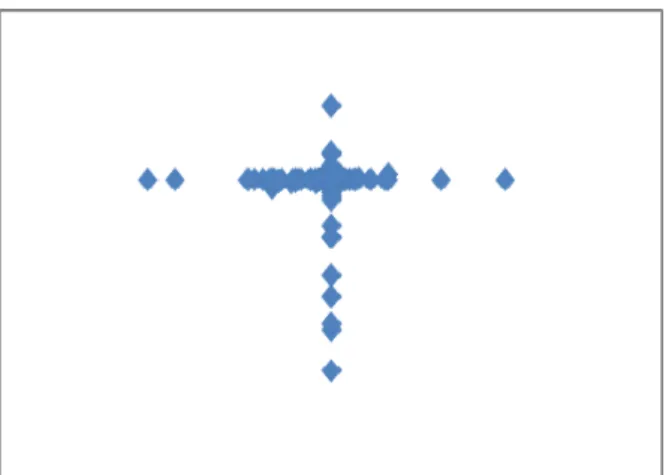
We have used kernel functions generated by polynomial and sigmoid functions to comparen their effectiveness in clustering data sets. We have taken hand-writing pen-digits data sets. We have used kernels generated by using polynomial functions and sigmoid functions and observed that there is not much difference in the actual clustering of data points, but the execution time for the sigmoid kernel functions is much less than the polynomial kernel function. The pen-digits data sets is downloaded from (ftp://ics.uci.edu/ pub/machine-learning-database/ pendigts), which contains <x,y> co-ordinates of the hand-written digits.. The results are shown in the diagrams.

(4)

Figure 2: Polynomail Kernal Graph with degree 5

7. Results

It is observed that the clusters generated by polynomial-based kernel and sigmoid-based kernel are complete different even-though time taken to generate the kernels is also different

Figure 3:Sigmoid kernel

8. Conclusion

In this paper a dimensionality reduction through kernel function was applied to leader’s algorithm. We have applied pen digits data compact and used a threshold value to fix the distance betweenthe centroids of the clusters. It is observed different kernel functions produce slightly varied clusters and the right clusters can be determined by the correct classification of new sets of data.

9. References

[1] Inderjit S. Dhillon, inderjit@cs.utexas.edu Yuqiang Guan yguan@cs.utexas.edu Brian Kulis kulis@cs.utexas.edu Kernel kmeans, Spectral Clustering and Normalized Cuts

[2] S. Dhillon, Y. Guan, and J. Kogan. Iterative clustering of high dimensional text data augmented by local search. In Proceedings of the 2002 IEEE International Conference on Data Mining, pages 131–138, 2002.

[3] S. Dhillon, E. M. Marcotte, and U. Roshan. Diametrical clustering for identifying anti-correlated gene clusters. [4] Bioinformatics, 19(13):1612–1619, September 2003.

[5] M. Girolami. Mercer kernel based clustering in feature

[6] Space. IEEE Transactions on Neural Networks, 13(4):669–688, 2002.

[7] G. Golub and C. Van Loan. Matrix Computations. Johns Hopkins University Press, 1989.

[8] R. Kannan, S. Vempala, and A. Vetta. On clustering’s –good, bad, and spectral. In Proceedings of the 41st Annual Symposium on Foundations of Computer Science, 2000.

[9] Y. Ng, M. Jordan, and Y. Weiss. On spectral clustering: Analysis and an algorithm. In Proc. of NIPS-14, 2001. [10] Sch¨olkopf, A. Smola, and K.-R. M¨uller. Nonlinear component analysis as a kernel eigenvalue problem. Neural [11] Computation, 10:1299–1319, 1998.

[12] J. Shi and J. Malik. Normalized cuts and image segmentation. IEEE Trans. Pattern Analysis and Machine Intelligence, 22(8):888–905, August 2000.

[13] S. X. Yu and J. Shi. Multiclass spectral clustering. In International Conference on Computer Vision, 2003.

[14] H. Zha, C. Ding, M. Gu, X. He, and H. Simon. Spectral relaxation for k-means clustering. In Neural Info. Processing Systems, 2001. [15] A new method for dimensionality Reduction using K-means clustering Algorithm for High Dimensional Data set D Napoleon, S.

Pavalakodi