Market Competitiveness Evaluation of Mechanical Equipment with a Pairwise Comparisons Hierarchical Model.

(1)

Market Competitiveness Evaluation of

Mechanical Equipment with a Pairwise

Comparisons Hierarchical Model

Fujun Hou*

School of Management and Economics, Beijing Institute of Technology, Beijing 100081, P.R. China *houfj@bit.edu.cn

Abstract

This paper provides a description of how market competitiveness evaluations concerning mechanical equipment can be made in the context of multi-criteria decision environments. It is assumed that, when we are evaluating the market competitiveness, there are limited number of candidates with some required qualifications, and the alternatives will be pairwise compared on a ratio scale. The qualifications are depicted as criteria in hierarchical struc-ture. A hierarchical decision model called PCbHDM was used in this study based on an analysis of its desirable traits. Illustration and comparison shows that the PCbHDM provides a convenient and effective tool for evaluating the market competitiveness of mechanical equipment. The researchers and practitioners might use findings of this paper in application of PCbHDM.

1 Introduction

The increasing complexity of the socio-economic environment makes it an important yet com-plicated task to evaluate the market competitiveness concerning mechanical equipment. The competitiveness evaluation of mechanical equipment includes many different objectives and reflects the wishes of wide-ranging interests, for example, in addition to the quality, the mechanical performance and the price, such influential factors as occupant comfort, ease of training and maintenance, as well as the environmental considerations have to be taken into account. The evaluation task comprises, therefore, a multi-criteria decision making problem involving some complicated even conflicting objectives or attributes.

During the past 35 years, the Analytic Hierarchy Process (AHP) developed by Saaty [1] has often been utilized to evaluate alternatives in multi-criteria decision environments (e.g., [2]). However, there have been a number of criticisms on Saaty’s AHP among which the rank rever-sal has attracted everlasting controversies among researchers. The rank reverrever-sal refers to a phenomenon that the ranking of alternatives produced by Saaty’s AHP may be altered by the addition or deletion of another independent alternative for consideration [3]. Dyer thus pointed out that the rankings produced by Saaty’s AHP is arbitrary [4]. Triantaphyllou also reported that the decision maker may never know the exact ranking of the alternatives in a OPEN ACCESS

Citation:Hou F (2016) Market Competitiveness Evaluation of Mechanical Equipment with a Pairwise Comparisons Hierarchical Model. PLoS ONE 11(1): e0146862. doi:10.1371/journal.pone.0146862

Editor:Yong Deng, Southwest University, CHINA

Received:August 14, 2015

Accepted:December 21, 2015

Published:January 19, 2016

Creative Commons Attribution License, which permits unrestricted use, distribution, and reproduction in any medium, provided the original author and source are credited.

Data Availability Statement:All relevant data are within the paper and its Supporting Information files.

Funding:The work was supported by the National Natural Science Foundation of China (No. 71571019). The funders had no role in study design, data collection and analysis, decision to publish, or preparation of the manuscript.

(2)

given multi-criteria decision-making (MCDM, for short) problem when the original AHP, or its current additive variants, are used [5].

Considering these possible shortcomings, this paper would not use Saaty’s AHP, instead, we used another hierarchical decision-making technique, specifically the pairwise comparisons based hierarchical decision model (PCbHDM, for short) [6,7], to evaluate the market competi-tiveness of mechanical equipment in a multi-criteria decision-making environment. The rea-son for our choice will be interpreted in more detail in Section 3.

The remainder of the paper is organized as follows. Section 2 provides a description of the problem. Section 3 describes how the decision-making method was selected. Section 4 includes illustration, comparison and discussion, and Section 5 contains our concluding remarks.

2 Description of the problem

Evaluation of market competitiveness of industrial products is fairly important in today’s highly competitive environment. Both the sellers and the buyers could benefit from the assess-ment based on which the sellers may improve their products and services for gaining the competitive advantage, and the buyers may purchase the product with highest degree of desir-ability. A careful market competitiveness evaluation system should cover all the criteria that buyers and sellers are interested in. In the development of such an evaluation system, the basic problem is to score and to rank a set of alternatives given some decision criteria. Therefore, the identification of criteria and integration of experts’assessments are two components of the evaluation system.

Let {A1,A2,. . .,Am} be the set of alternatives and {c1,c2,. . .,cn} be the set of criteria according

to which the desirability of an alternative is to be compared. The purpose of the evaluation pro-cess is a quantitative comparison among the available alternatives in the context of a multi-cri-teria decision environment. In the mechanical equipment evaluation system, the alternatives refer to the machines having same functions but coming from different producers. The criteria stand for the concerns both of the sellers and the buyers.

3 Selection of decision-making method

3.1 Pairwise comparison matrices

Denote byX= {x1,x2,. . .,xn} the object (alternative or criterion) set. A pairwise comparison

matrix (PCM, for short) over the objective set is an useful tool for deriving object weights or priorities, where the component can be assumed of different meanings as described in the following.

Multiplicative type:[1] For anbynPCMM= (pij) with8i,j(pij2(0,+1)), the conditions of

reciprocity and consistency are given by8i,j(pijpji= 1) and8i,j,k(pijpjk=pik), respectively.

The componentpijrepresents the preference ratio of objectxioverxj. For a consistent

multi-plicative PCMM= (pij), an×1 vectorW= (ω_k) withω_k>0, is called a priority vector ofM

such that8i,j2I,pijω_j=ω_i.

Fuzzy type:[8] For anbynPCMF= (fij) with8i,j(fij2[0, 1]), the conditions of reciprocity and

consistency are given by8i,j(fij+fji= 1) and8i,j,k(fij+fjk=fik−0.5), respectively. The component fijrepresents the preference degree of objectxioverxj. For a consistent fuzzy PCMF= (fij),

an× 1 vectorW= (ω_k) is called a priority vector ofFsuch that8i,j2I,f_ij=ω_i₋ω_j+0.5.

(3)

3.2 Saaty

’

s AHP and related issues

Saaty’s AHP is one of the extensively used MCDM techniques. Application of the AHP involves the following steps [1]:

Step 1:Structure the decision problem as a hierarchy of elements (goal, criteria, and

alternatives).

Step 2:Make pairwise comparison of elements at each level of the hierarchy with respect to

each criterion on the preceding level and obtain the PCM.

Step 3:Compute the consistency ratio of the PCM to determine whether it satisfies a

consis-tency test. If it does not have acceptable consisconsis-tency, go back to Step 2 and redo the pairwise comparisons.

Step 4:Calculate the local priorities of the decision elements by means of the right eigenvector

approach.

Step 5:Synthesize the local priorities across various levels by using an additive aggregation rule

to obtain the final priorities of alternatives.

Saaty presented two modes of his AHP, one is called the original mode where the local pri-orities are all sum-normalized (by summing to unity), and the other is called the ideal mode where the alternative’s local priorities are max-normalized (by dividing each component by the largest component).

Though widely used, the AHP has also suffered from a number of controversies including, among others,

(1) Rank reversal: A phenomenon that the ranking of alternatives may be altered by the addi-tion or deleaddi-tion of another independent alternative for consideraaddi-tion [3,4].

We consider the Dyer’s example for illustration. There are 4 alternatives (say A,B,C,D) to be evaluated with respect to three criteria (say a,b,c) having equal importance weights. The data is provided as (ratio-scale measurements)

a b c A

B C D

1 9 8

9 1 9

1 1 1

8 1 8

:

Using the original AHP, when we just evaluate A, B and C, we obtainAB; while we evaluate A, B, C and D, the rank is reversed since we obtainA B.

As pointed out in [3] and [13], neither the original AHP nor the ideal AHP has the prop-erty of rank preservation. As a result, the ranking produced by Saaty’s AHP is arbitrary [4], and we may never know the exact ranking if we use the original AHP or its current additive variants [5].

(4)

have its isomorphic counterpart used for other type of preference information e.g. for the difference information [18].

Here we point out yet another one:

(3) The paradox of the consistency criterion: For a multiplicative PCM, Saaty defined the con-sistency index byC.I. = (λmax)/(n−1), whereλmaxis the principal eigenvalue of the

consid-ered PCM andnis its order. For checking acceptable consistency, Saaty proposed a 0.1 threshold for the consistency ratio, namely,C.R.0.1, whereC.R. =C.I./R.I. andR.I. is the average value of theC.I. obtained from 500 PCMs whose entries were randomly generated using the 1 to 9 scale. As a frequently used criterion of cardinal consistency, however, it may lead to a paradox: if a PCM ofC.R. = 0.1 is acceptable, then, we have no reason to reject a PCM ofC.R. = 0.1 + 10−10_{; and then, a PCM of}_C_._R_{. = 0.1 + 2 × 10}−10_{is also acceptable;}_{. . .}_; thus, any a PCM is acceptable, and thus we reach a paradox. This paradox resembles the paradox of the heap (also referred to as the‘Sorites paradox’, sorites being the Greek word for heap). Moreover, Saaty’s criterion has no counterparts for other kinds of PCM.

3.3 The PCbHDM and desirable traits

The PCbHDM is another hierarchical decision model different from the Saaty’s AHP. In this subsection, we introduce the steps, the foundations and desirable traits of the PCbHDM [6,7].

3.3.1 Steps. The following steps are suggested for applying the PCbHDM:

Step 1:Break down the decision problem into a hierarchy of decision elements (goal as the top

level, criteria and sub-criteria as the middle levels, and alternatives as the terminal level);

Step 2:Establish the multiplicative PCMs based on a ratio scale for the decision elements in

each level of the hierarchy with respect to one decision element at a time in the immediate upper level.

Step 3:Determine whether or not the PCMs have acceptable consistency by

Ifaik<ajk; then; 8lðailajlÞ: ð1Þ

If not, go back to Step 2 and redo the pairwise comparisons.

Step 4:Derive the normalized local weight vectors from the PCMs using the row geometric

mean method

o_i¼ ðQn j¼1a_ijÞ

1

n: ð2Þ

If a local weight vector is of the criteria(sub-criteria) in a same level with respect to a speciﬁc decision element in the immediate upper level, it is then to be sum-normalized; if it is of the alternatives with respect to a terminal criterion, it is then to be min-normalized (by dividing each component by the smallest component).

Step 5:Compute the terminal sub-criteria (criteria) weights with respect to the total goal using

the Hierarchy Composition Rule

b_jðlþ1Þ¼b_kðlÞbðjlþ1Þ; ð3Þ

where

(5)

• bðjlþ1Þdenotes the global weight of the sub-criterion w.r.t. the total goal;

• bð_klÞdenotes the father-criterion’s weight w.r.t. the total goal.

Step 6:To get an overall priority for each alternative, synthesize the alternative’s local weights using the weighted geometric mean aggregation rule

rj¼ Qm

l¼1u

bl

jl ð4Þ

where,_ujlis the alternative’s local weight (has been min-normalized in Step 4) w.r.t. the ter-minal sub-criterion, and,β_lis the terminal sub-criterion’s weight w.r.t. the total goal.

3.3.2 Foundations. Weighted means are frequently used as aggregation rules in MCDM

problems. When the weighted mean is used in a MCDM problem, the problem can be decom-posed or incorporated, e.g.,

30:2

50:3

90:5

Ð ð3_Þ0:2_ð50:3=0:8

90:5=0:8

Þ0:8 ;

and

0_:23_þ0_:35_þ0_:59_Ð0_:2_ð3_{Þ þ}0_:8_ð0_:3₌0_:85_þ0_:5₌0_:89_Þ_:

We show this below by two theorems.

Theorem 3.1Suppose that the decision matrix of a MCDM problem isD¼ ðuijÞnmwhere

8i;jðuij>0Þ, and that the criteria weight vector isB= (βl)m×1whereβl>0 andPml¼1bl ¼1. If

the weighted geometric mean is used for the aggregation, we have

Ym

l¼1

ujl bl

Ð Y

t

l¼1

ujl

b_l Pt

i¼1bi 0

B @

1

C A

Pt i¼1bi

Ym

l¼tþ1

ujl

b_l Pm

i¼tþ1b_i 0

B @

1

C A

Pm i¼tþ1bi

;

j¼1_;2_;. . ._;_n_:

Theorem 3.2Suppose that the decision matrix of a MCDM problem isD¼ ðuijÞnmwhere

8i;jðuij0Þ, and that the criteria weight vector isB= (βl)m×1whereβl>0 andP m

l¼1bl ¼1. If

the weighted arithmetic mean is used for the aggregation, we have

Xm

l¼1 b_l ujl

Ð ðPt

i¼1biÞ Xt

l¼1 b_l Pt

i¼1b_i

ujl

þ ðXm

i¼tþ1biÞ Xm

l¼tþ1 b_l Pm

i¼tþ1bi

ujl

;

j¼1_;2_;. . ._;_n_:

The above two theorems do hold since we just rewrite the weighted means in other forms. However, these two theorems provide a foundation for hierarchical decision models in that they tell WHEN and HOW a MCDM problem can be decomposed or incorporated:

• If the criteria’weights w.r.t. the total goal are sum-normalized, then, the MCDA problem can be decomposed (the left-to-right means decomposition, i.e., one level to multi-level).

• If the weights of the same level sub-criteria dominated by the same immediate upper level criterion are sum-normalized, then, the decision problem can be incorporated (the right-to-left means incorporation, i.e., multi-level to one level).

(6)

Letbðjlþ1Þdenote the local weight of a sub-criterion in levell+1 w.r.t. its immediately

preceding criterion/sub-criterion in levell(called the father-criterion);

Letbð_jlþ1Þdenote the global weight of the sub-criterion w.r.t. the total goal;

Letbð_klÞdenote the father-criterion’s weight w.r.t. the total goal.

Then, the Hierarchy Composition Rule is

b_jðlþ1Þ ¼b_kðlÞbðjlþ1Þ:

Specifically, the Theorem 3.1 presents a foundation for the PCbHDM in that the weighted geometric mean is used as the aggregation rule.

3.3.3 Desirable traits. The PCbHDM is a hierarchical model that overcomes the

afore-mentioned issues related to the AHP:

1. About the rank reversal: It can be easily proved that the weighted geometric mean aggrega-tion rule used in the PCbHDM is a rank preserved aggregaaggrega-tion rule (see [19] or [20]). For a quick understanding, we again consider the Dyer’s example but in a more general way:

• the alternatives A,B,C,D are renamed asA1,A2,A3,A4, respectively;

• the criteria a,b,c are renamed asC1,C2,C3, respectively;

• letω₁,ω₂,ω₃denote the criteria weights;

• letyijdenote the alternativeAi’s local priority under criterionCj, wherei= 1,2,3,4, and,

j= 1,2,3 (We’ll give an interpretation onyijjust below);

• theAi’s global priorities provided by Saaty’s AHP before and afterA4’s addition are

denoted byAHP(Ai) andAHP+(Ai), respectively;

• theAi’s global priorities provided by the PCbHDM before and afterA4’s addition are

denoted byPCbHDM(Ai) andPCbHDM+(Ai), respectively.

Here we give a further interpretation on the notationyij, namely, the local priority of

alter-nativeAiunder criterionCj. In Dyer’s example [4] as well as in Belton-Gear’s example [3],

the local priorities are derived from consistent PCMs. It is known that, a consistent PCM corresponds to numerous prority vectors, which are unique up to multiplication by a posi-tive constant. Moreover, any column e.g. the first column of a consistent PCM can be taken as one of its priority vectors, sinceω_i=ω_jp_ij[12]. We denote byðpj

ikÞ33the

consis-tent PCM of alternatives with respect to criterionCjbefore the addition of alternativeA4,

and byðpj

ikÞ44the consistent PCM of alternatives with respect to criterionCjafter the

addition. BecauseA4is added as an independent alternative, we thus havep j

ik ¼p

j ikfori,j,

k= 1,2,3. As already mentioned, we can take any column as the local priority vector to be derived from a consistent PCM. For the convenience of discussion, we will take the first column for our purpose, since in Dyer’s example, the first column ofðpj_ikÞ33is included

also in the firsrt column ofðpj

ikÞ44. Therefore we have:yij¼p j

i1¼p

j

i1;i¼1;2;3; and yij¼pj_i1;i¼4. For conciseness we just use the notationyijto indicate the alternatives’

local priorities in the following illustration.

(7)

A4is added:

AHPðA1Þ

AHPðA2Þ

¼o1ðy11= P3

i¼1y_i1Þ þo2ðy12= P3

i¼1y_i2Þ þo3ðy13= P3

i¼1y_i3Þ o1ðy21=

P3

i¼1yi1Þ þo2ðy22= P3

i¼1yi3Þ

and

AHPþ_ð_A 1Þ

AHPþ_ð_A 2Þ

¼o1ðy11= P4

i¼1yi3Þ o1ðy21=

P4

i¼1yi3Þ :

Because Saaty’s AHP uses the above sum-normalization and additive aggregation, when we

haveAHPðA1Þ

AHPðA2Þ<1we do not deﬁnitely have

AHPþ_ð_A_1Þ

AHPþ_ð_A_2Þ<1, and thus the rank reversal

may happen as shown by Dyer’s example.

Comparatively, if we use the PCbHDM, the ratios are provided as:

PCbHDMðA1Þ

PCbHDMðA2Þ

¼

ðy11=minfy_i1ji¼1;2;3gÞ

o1

o2

o3

ðy21=minfyi1ji¼1;2;3gÞ

o1

o2

o3

and

PCbHDMþ_ð_A 1Þ

PCbHDMþ_ð_A 2Þ

¼

ðy11=minfyi1ji¼1;2;3;4gÞ

o1

o2

o3

ðy21=minfy_i1ji¼1;2;3;4gÞ

o1

o2

o3

:

Clearly, we havePCbHDM_PCbHDMð_ðA_A1Þ_2Þ¼PCbHDMþðA1Þ PCbHDMþ_ð_A_2Þ¼

ðy11Þo1 ðy12Þo2

ðy13Þo3 ðy21Þo1

ðy22Þo2

ðy23Þo3. Therefore, the PCbHDM preserves not only the rank but also the ratio. It is a hierarchical decision model immune to rank reversal.

It is worth noticing that: (1) Although the above discussion is carried out on a hierarchy with just one criterion-level involved, the verdict that the PCbHDM is a hierarchical deci-sion model immune to rank reversal is also suitable to multiple levels, since the multi-level can be transformed into one-level according to Theorem 3.1; (2) The rank reversal is dis-cussed in the context that, as done in Belton-Gear’s example as well as in Dyer’s example, the involved PCMs are all consistent. Otherwise, rank preservation may not be expected, since inconsistency means judgment contradiction and anything may happen.; (3) The AHP’s rank reversal, which is observed even in perfect consistency cases, is one of the main reasons why many researchers think the AHP as a doubtful method. Comparatively, the PCbHDM can be proven mathematically that the rank reversal is avoided provided that all the involved PCMs are consistent; (4) Rank preservation is not always guaranteed by the PCbHDM when inconsistent PCMs are involved. We shall show this in the illustration section.

2. About the paradox of Saaty’s consistency criterion: Since the acceptable consistency crite-rion used in the PCbHDM is an ordinal transitivity rather than a cardinal one, thus, the par-adox is avoided. Moreover, it has isomorphic counterparts in other cases of PCM [6,7].

(8)

In accordance with the above considerations, the present work selects the PCbHDM as the decision making method. The PCbHDM’s desirable traits assure its suitability to the applica-tion of this study.

We should note that the main features of PCbHDM are based on previous work of many researchers including, not limited to: the pairwise comparison technique can be traced to at least as early as Thurstone’s work [21]; the hierarchical MCDM model can be traced to Miller’s work [22]; the min-normalization of the multiplicative PCM was suggested in [23]; the

weighted geometric aggregation rule was supported by [19,24] and many others; using the geo-metric mean to derive weights from a multiplicative PCM was supported by [19], [24,25], also by many others; the mapping between a multiplicative PCM and a fuzzy PCM was first dis-cussed in [10] and successive studies were also conducted in [9] and [11]; PCM’s isomorphic correspondence from the prospective of abstract algebra was discussed by some researchers as can be seen in [12,20,26,27].

4 Illustration, comparison and discussion

This section includes case studies aiming at (1) illustrating the evaluation process using the selected method; (2) showing that the PCbHDM does not guarantee rank preservation when inconsistent PCMs are involved; and (3) showing that the PCbHDM preserves the rank when the involved PCMs are all consistent, while the AHP does not. The example is modified from a real-world example presented in [28]. A graphical software tool has been developed to allow an easy data input and a direct results output. There are 5 alternatives (denoted byA1,A2,A3,A4

andA5) to be assessed by five experts comprising a decision group responsible for constructing

the criteria structure and determining the input data through a Delphi process. We shall make a comparision between the results provided by the PCbHDM and the AHP. To permit a con-trast comparison to be analyzed, we shall list the results calculated by the two methods in same tables.

4.1 Illustration

4.1.1 Criteria hierarchy. Market competitiveness is related to intangible benefits and

indi-rect costs. The evaluation process may involve social, technical, economic, service, and envi-ronmental factors (criteria). The decision group identifies seven influential factors including mechanical behavior, price, use cost, operating comfort, service quality, quality and reputation, and safety and environment, which include 18 sub-factors.Table 1shows the criteria selected for this analysis, andFig 1shows the hierarchy structure.

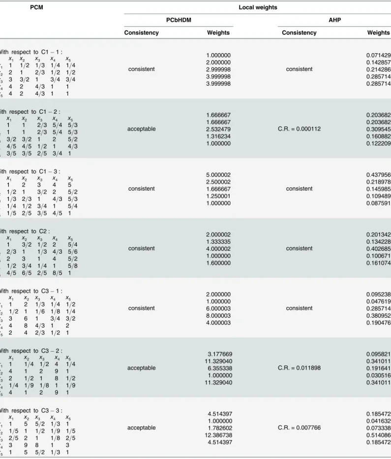
4.1.2 Pairwise comparison data. The input data are presented by the decision group as

multiplicative PCMs as shown by the‘PCM’columns of Tables2,3and4.

4.1.3 Local weights and global weights. Now, we find the overall priorities of alternatives

by implementing the PCbHDM procedure described in Subsection 3.3.1:

• The PCM’s acceptable consistency is tested by the criterion of inequalityEq (1), the local weighs are derived byEq (2)and are provided in Tables2,3and4. We should note that the criterion’s local weights are sum-normalized, and, the alternative’s local weights are min-normalized.

(9)

• From the aggregation rule ofEq (4), we obtain the alternatives’overall priorities as: 2.588777, 2.325968, 2.829265, 2.667508, 2.884724.

Thus, the alternative’s ranking produced by the PCbHDM is:

A5 A3 A4 A1A2: ð5 aÞ

4.1.4 Comparison. To highlight the procedure of the suggested model and to make a

com-parison, we list the results following the Saaty’s original AHP. They are also included in Tables

2–4. By Saaty’s original AHP, the alternatives’overall priorities are obtained as: 0.176182, 0.182554, 0.207429, 0.236312, 0.197525, which indicate a final ranking

A4A3A5A2A1: ð5 bÞ

Now, we further investigate what will happen if we delete an existing alternative while the comparison results between the other ones remain unchanged. For instance, we delete the Table 1. Criteria and sub-criteria.

Criteria Sub-criteria

C1: Mechanical behavior C1-1: Productivity

C1-2: Exactitude C1-3: Versatility C2: Price

C3: Use cost C3-1: Durability

C3-2: Maintenance cost C3-3: Fuel consumption

C4: Operating comfort C4-1: Operability

C4-2: Ride comfort C4-3: Cab noise C4-4: Visibility

C5: Service quality C5-1: Pre-sales & Sales training

C5-2: Service convenience

C6: Quality & reputation C6-1: Lead-edge technologies

C6-2: Quality

C6-3: Product appearance

C7: Safety & environment C7-1: Safety

C7-2: Noise C7-3: Emission doi:10.1371/journal.pone.0146862.t001

Fig 1. The criteria hierarchy.

(10)

Table 2. PCM of criteria with respect to the goal and local weights.

PCM Local weights

PCbHDM AHP

Consistency Weights Consistency Weights

1 3/2 4/3 8/5 2 3/2 3

acceptable

0.220561

C.R. = 0.000579

0.220497

2/3 1 8/9 9/8 4/3 1 2 0.148163 0.148095

3/4 9/8 1 6/5 3/2 9/8 9/4 0.165421 0.165373

5/8 8/9 5/6 1 5/4 8/9 3/2 0.131510 0.131686

1/2 3/4 2/3 4/5 1 3/4 3/2 0.110281 0.110249

2/3 1 8/9 9/8 4/3 1 2 0.148163 0.148095

1/3 1/2 4/9 2/3 2/3 1/2 1 0.075902 0.076006

doi:10.1371/journal.pone.0146862.t002

Table 3. PCMs of sub-criteria with respect to criteria and local weights.

PCM Local weights

PCbHDM AHP

With respect to C1 :

C1 1 C1 2 C1 3

C1 1 1 1 2

C1 2 1 1 2

C1 3 1=2 1=2 1

consistent

0:400000 0:400000

0:200000 consistent

0:400000 0:400000 0:200000

C3 1 C3 2 C3 3

C3 1 1 1 3=4

C3 2 1 1 3=4

C3 3 4=3 4=3 1

consistent

0:300000 0:300000

0:400000 consistent

0:300000 0:300000 0:400000

C4 1 C4 2 C4 3 C4 3

C4 1 1 3=2 3=2 1

C4 2 2=3 1 1 2=3

C4 3 2=3 1 1 2=3

C4 4 1 3=2 3=2 1

consistent

0:300000 0:200000 0:200000 0:300000

consistent

0:300000 0:200000 0:200000 0:300000

C5 1 C5 2

C5 1 1 1=4

C5 2 4 1

consistent

0:200000

0:800000 _consistent

0:200000 0:800000

C6 1 C6 2 C6 3

C6 1 1 3=5 3=2

C6 2 5=3 1 5=2

C6 3 2=3 2=5 1

consistent

0:300000 0:500000

0:200000 consistent

0:300000 0:500000 0:200000

C7 1 C7 2 C7 3

C7 1 1 4=3 4=3

C7 2 3=4 1 1

C7 3 3=4 1 1

consistent

0:400000 0:300000

0:300000 consistent

0:400000 0:300000 0:300000

(11)

Table 4. PCMs of alternatives with respect to terminal criteria and local weights.

PCM Local weights

PCbHDM AHP

With respect to C1 1 : x₁ x₂ x₃ x₄ x₅ x₁ ₁ ₁₌₂ ₁₌₃ ₁₌₄ ₁₌₄ x₂ 2 1 2=3 1=2 1=2 x₃ 3 3=2 1 3=4 3=4 x

4 4 2 4=3 1 1

x₅ 4 2 4=3 1 1

consistent

1:000000 2:000000 2:999998 3:999998 3:999998

consistent

0:071429 0:142857 0:214286 0:285714 0:285714

With respect to C1 2 : x₁ x₂ x₃ x₄ x₅ x₁ 1 1 2=3 5=4 5=3 x₂ 1 1 2=3 5=4 5=3 x

3 3=2 3=2 1 2 5=2

x₄ 4=5 4=5 1=2 1 4=3 x₅ ₃₌₅ ₃₌_{5 2}₌₅ ₃₌₄ ₁

acceptable

1:666667 1:666667 2:532479 1:316234 1:000000

C.R. = 0.000112

0:203682 0:203682 0:309545 0:160882 0:122209

With respect to C1 3 : x₁ x₂ x₃ x₄ x₅ x₁ ₁ ₂ ₃ ₄ ₅ x

2 1=2 1 3=2 2 5=2

x₃ 1=3 2=3 1 4=3 5=3 x₄ ₁₌_{4 1}₌_{2 3}₌_{4 1} ₅₌₄ x₅ 1=5 2=5 3=5 4=5 1

consistent

5:000002 2:500002 1:666667 1:250001 1:000000

consistent

0:437956 0:218978 0:145985 0:109489 0:087591

With respect to C2 : x₁ x₂ x₃ x₄ x₅ x

1 1 3=2 1=2 2 5=4

x₂ 2=3 1 1=3 4=3 5=6 x₃ ₂ ₃ ₁ ₄ ₅₌₂ x₄ 1=2 3=4 1=4 1 5=8 x₅ 4=5 6=5 2=5 8=5 1

consistent

2:000002 1:333335 4:000002 1:000000 1:600000

consistent

0:201342 0:134228 0:402685 0:100671 0:161074

With respect to C3 1 : x

1 x2 x3 x4 x5

x₁ 1 2 1=3 1=4 1=2 x₂ ₁₌_{2 1} ₁₌_{6 1}₌_{8 1}₌₄ x₃ 3 6 1 3=4 3=2 x₄ 4 8 4=3 1 2 x

5 2 4 2=3 1=2 1

consistent

2:000000 1:000000 6:000003 8:000003 4:000003

consistent

0:095238 0:047619 0:285714 0:380952 0:190476

With respect to C3 2 : x₁ x₂ x₃ x₄ x₅ x₁ ₁ ₁₌_{4 1}₌_{2 4} ₁₌₄ x₂ 4 1 2 9 1 x₃ 2 1=2 1 8 1=2 x

4 1=4 1=9 1=8 1 1=9

x₅ 4 1 2 9 1

acceptable

3:177669 11:329040 6:355338 1:000000 11:329040

C.R. = 0.011898

0:095821 0:341011 0:191641 0:030516 0:341011

With respect to C3 3 : x₁ x₂ x₃ x₄ x₅ x₁ 1 5 5=2 1=3 1 x₂ 1=5 1 1=2 1=9 1=5 x

3 2=5 2 1 1=8 2=5

x₄ 3 9 8 1 3 x₅ ₁ ₅ ₅₌₂ ₁₌₃ ₁

acceptable

4:514397 1:000000 1:782602 12:386738 4:514397

C.R. = 0.007766

0:185472 0:041632 0:073338 0:514086 0:185472

(12)

Table 4. (Continued₎

PCM Local weights

PCbHDM AHP

With respect to C4 1 : x₁ x₂ x₃ x₄ x₅ x₁ 1 4 4 1=2 5 x₂ 1=4 1 1 1=8 5=4 x

3 1=4 1 1 1=8 5=4

x₄ 2 8 8 1 9 x₅ ₁₌₅ ₄₌_{5 4}₌₅ ₁₌₉ ₁

acceptable

4:895740 1:223936 1:223936 9:587312 1:000000

C.R. = 0.000298

0:272964 0:068241 0:068241 0:534774 0:055781

With respect to C4 2 : x₁ x₂ x₃ x₄ x₅ x₁ 1 1=4 1=2 2 1=5 x

2 4 1 2 8 4=5

x₃ 2 1=2 1 4 2=5 x₄ ₁₌₂ ₁₌₈ ₁₌₄ ₁ ₁₌₉ x₅ 5 5=4 5=2 9 1

acceptable

1:958294 7:833181 3:916592 1:000000 9:587306

C.R. = 0.000298

0:080588 0:322354 0:161177 0:041171 0:394710

With respect to C4 3 : x₁ x₂ x₃ x₄ x₅ x

1 1 1=2 1=5 1=4 2

x₂ 2 1 2=5 1=2 4 x₃ ₅ ₅₌_{2 1} ₅₌_{4 9} x

4 4 2 4=5 1 8

x₅ 1=2 1=4 1=9 1=8 1

acceptable

1:958294 3:916592 9:587306 7:833181 1:000000

C.R. = 0.000298

0:080588 0:161177 0:394710 0:322354 0:041171

1 x2 x3 x4 x5

x₁ 1 8 6 1=2 4 x₂ ₁₌_{8 1} ₃₌_{4 1}₌_{9 1}₌₂ x₃ 1=6 4=3 1 1=8 2=3 x₄ 2 9 8 1 8 x

5 1=4 2 3=2 1=8 1

acceptable

7:130401 1:000000 1:288786 11:720609 1:782599

C.R. = 0.009159

0:309362 0:043626 0:055808 0:513864 0:077341

With respect to C5 1 : x₁ x₂ x₃ x₄ x₅ x₁ ₁ ₅ ₃ ₂ ₈ x₂ 1=5 1 3=5 2=5 8=5 x₃ 1=3 5=3 1 2=3 8=3 x

4 1=2 5=2 3=2 1 4

x₅ 1=8 5=8 3=8 1=4 1

consistent

8:000011 1:600002 2:666671 4:000005 1:000000

consistent

0:463320 0:092664 0:154440 0:231660 0:057915

With respect to C5 2 : x₁ x₂ x₃ x₄ x₅ x₁ 1 1=5 1=2 4 1=4 x₂ 5 1 5=2 9 5=4 x

3 2 2=5 1 8 1=2

x₄ 1=4 1=9 1=8 1 1=8 x₅ ₄ ₄₌_{5 2} ₈ ₁

acceptable

2:968218 12:650521 5:936440 1:000000 10:335940

C.R. = 0.020287

0:090406 0:384911 0:180811 0:031062 0:312810

1 x2 x3 x4 x5

x₁ 1 1=2 3 4 1 x₂ ₂ ₁ ₆ ₈ ₂ x₃ 1=3 1=6 1 4=3 1=3 x₄ ₁₌₄ ₁₌_{8 3}₌₄ ₁ ₁₌₄ x₅ 1 1=2 3 4 1

consistent

4:000003 8:000006 1:333335 1:000000 4:000003

consistent

0:218182 0:436364 0:072727 0:054545 0:218182

(13)

alternativeA4, and therefore, the PCMs of alternatives with respect to the terminal criteria are

obtained by deleting the 4th rows and the 4th columns of the PCMs contained inTable 4. The PCbHDM gives an overall priorities as: 2.064422, 1.855985, 2.228957, 2.341745, which indicate a final ranking

A5A3A1A2: ð6 aÞ

Table 4. (Continued₎

PCM Local weights

PCbHDM AHP

With respect to C6 2 : x₁ x₂ x₃ x₄ x₅ x₁ 1 4 4 1=4 1=2 x₂ 1=4 1 1 1=9 1=8 x

3 1=4 1 1 1=9 1=8

x₄ 4 9 9 1 2 x₅ ₂ ₈ ₈ ₁₌₂ ₁

acceptable

3:565204 1:000000 1:000000 11:329050 7:130411

C.R. = 0.011898

0:147416 0:041423 0:041423 0:474906 0:294833

With respect to C6 3 : x₁ x₂ x₃ x₄ x₅ x₁ 1 1=4 1=2 1=4 1=2 x

2 4 1 2 1 2

x₃ 2 1=2 1 1=2 1 x₄ ₄ ₁ ₂ ₁ ₂ x₅ 2 1=2 1 1=2 1

consistent

1:000000 4:000002 2:000002 4:000002 2:000002

consistent

0:076923 0:307692 0:153846 0:307692 0:153846

With respect to C7 1 : x₁ x₂ x₃ x₄ x₅ x

1 1 1=5 1=2 2 1=4

x₂ 5 1 5=2 9 5=4 x₃ ₂ ₂₌_{5 1} ₄ ₁₌₂ x

4 1=2 1=9 1=4 1 1=8

x₅ 4 4=5 2 8 1

acceptable

1:958294 9:587306 3:916592 1:000000 7:833181

C.R. = 0.000298

0:080588 0:394710 0:161177 0:041171 0:322354

1 x2 x3 x4 x5

x₁ 1 2 1=2 1 2 x₂ ₁₌_{2 1} ₁₌_{4 1}₌_{2 1} x₃ 2 4 1 2 4 x₄ 1 2 1=2 1 2 x

5 1=2 1 1=4 1=2 1

consistent

2:000000 1:000000 4:000002 2:000000 1:000000

consistent

0:200000 0:100000 0:400000 0:200000 0:100000

With respect to C7 3 : x₁ x₂ x₃ x₄ x₅ x₁ ₁ ₄ ₂ ₁₌₂ ₄ x₂ 1=4 1 1=2 1=8 1 x₃ 1=2 2 1 1=4 2 x

4 2 8 4 1 8

x₅ 1=4 1 1=2 1=8 1

consistent

4:000002 1:000000 2:000002 8:000005 1:000000

consistent

0:250000 0:062500 0:125000 0:500000 0:062500

(14)

In contrast, the original AHP produces an overall priorities as: 0.251942, 0.219854, 0.260724, 0.267482, which indicate a final ranking as

A5A3 A1A2: ð6 bÞ

Comparing Eqs(5-a)and(6-a), we know that the rank is preserved when the PCbHDM is used. As indicated by Eqs(5-b)and(6-b), rank reversals are observed for the original AHP, since the rank ofA1andA2and the rank ofA3andA5are reversed before and after the

alterna-tiveA4is deleted.

Let us further investigate what happens if repeating the test for each single alternatives,A1,

A2,A3andA5. We provide the results inTable 5.

As indicated byTable 5, the PCbHDM does not always preserve the rank. The reason lies in that some of the involved PCMs are inconsistent. Indeed, if all the PCMs are consistent, the PCbHDM will, as already proved in subsection 3.3.3, always preserve the rank. We show this below by providing the earlier hierarchy with consistent PCMs.

4.2 Rank preservation test with PCMs all consistent

In this subsection, we conduct a rank preservation test on the previous hierarchy with all the PCMs consistent and then we give a discussion. The data are prepared by modifying the incon-sistent PCMs based upon their respective first columns. For sake of conciseness, the input data and the intermediate results are relegated to the file of supplementary materials for this paper (S1andS2Files) and here we just list the final results and give a discussion.

4.2.1 Results. After converting the inconsistent PCMs into consistent ones based on their

respective first columns, and doing the rank preservation test for each single alternative, we obtain the results by the AHP and by the PCbHDM as shown in Tables6and7.

Table 5. Rank order for each single deletion.

Deleted alternative AHP PCbHDM

Rank order Preserve or not Rank order Preserve or not

None A₄ A₃ A₅ A₂ A₁ _– A₅ A₃ A₄ A₁ A₂ _–

A₁ A₄ A₅ A₂ A₃ _No A₅ A₄ A₃ A₂ _No

A₂ A₄ A₅ A₃ A₁ No A₅ A₄ A₃ A₁ No

A₃ A₄ A₅ A₂ A₁ Yes A₅ A₄ A₁ A₂ Yes

A₄ A₅ A₃ A₁ A₂ _No A₅ A₃ A₁ A₂ _Yes

A₅ A₄ A₃ A₂ A₁ _Yes A₃ A₄ A₁ A₂ _Yes

doi:10.1371/journal.pone.0146862.t005

Table 6. Rank order with a single alternative deleted (consistent case).

Deleted alternative AHP PCbHDM

Rank order Preserve or not Rank order Preserve or not

None A₄ A₅ A₂ A₃ A₁ _– A₅ A₄ A₃ A₁ A₂ _–

A₁ A₄ A₅ A₂ A₃ _Yes A₅ A₄ A₃ A₂ _Yes

A₂ A₄ A₅ A₃ A₁ _Yes A₅ A₄ A₃ A₁ _Yes

A₃ A₄ A₅ A₂ A₁ Yes A₅ A₄ A₁ A₂ Yes

A₄ A₅ A₁ A₃ A₂ No A₅ A₃ A₁ A₂ Yes

A₅ A₄ A₂ A₃ A₁ _Yes A₄ A₃ A₁ A₂ _Yes

(15)

4.2.2 Discussion. As shown byTable 6, the PCbHDM preserves the rank when the PCMs are all consistent. However, the AHP does not preserve the rank. Moreover, as indicated by

Table 7, the PCbHDM also preserves the ratios, e.g., the ratios of the global weights ofA1and

A2before and after theA4’s deletion are

2_:756191

2_:601603¼1:059420288and

2_:134666

2_:014938¼1:059420191;

respectively. These two ratios are identical to each other with a precision of 10−6_{. The} observa-tion that the AHP behaves rank reversal even in consistent case conﬁrms what the Dyer’s paper and the Triantaphyllou’s paper already illustrate:‘the ranking produced by Saaty’s AHP is arbitrary‘[4], and‘we may never know the exact ranking if we use the original AHP’[5].

5 Concluding remarks

This paper has described how a hierarchical decision-making technique, specifically pairwise-comparison-based hierarchical decision model (PCbHDM) could be used to make decisions regarding market competitiveness evaluations of mechanical equipment. The PCbHDM is a hierarchical decision model of the property of rank preservation. This desirable trait has been Table 7. Global weights with a single alternative deleted (consistent case).

Deleted alternative Global weights

AHP PCbHDM

None

A₁_{: 0:175333} A₁_{: 2:756191}

A₂_{: 0:187937} A₂_{: 2:601603}

A₃: 2:807889 A₃: 2:807889

A₄: 0:255357 A₄: 3:104646

A₅: 0:200337 A₅: 3:214869

A₁

A₂_{: 0:229391} A₂_{: 2:302583}

A₃: 0:220757 A₃: 2:485160

A₄: 0:315869 A₄: 2:747810

A₅: 0:233982 A₅: 2:845364

A₂

A₁_{: 0:216874} A₁_{: 2:513930}

A₃: 0:228857 A₃: 2:561084

A₄: 0:287943 A₄: 2:831758

A₅: 0:266325 A₅: 2:932293

A₃

A₁_{: 0:214649} A₁_{: 2:756190}

A₂: 0:233211 A₂: 2:601601

A₄: 0:306330 A₄: 3:104647

A₅: 0:245809 A₅: 3:214868

A₄

A₁_{: 0:257431} A₁_{: 2:134666}

A₂: 0:226750 A₂: 2:014938

A₃: 0:239426 A₃: 2:174706

A₅: 0:276392 A₅: 2:489912

A₅

A₁_{: 0:209352} A₁_{: 2:535070}

A₂: 0:250243 A₂: 2:392883

A₃: 0:228092 A₃: 2:582620

A₄: 0:312312 A₄: 2:855571

(16)

proved mathematically and shown in illustration through comparison. It is hoped that the PCbHDM finds applications in other multi-criteria decision environments.

When to cope with the AHP’s drawbacks, the PCbHDM concentrates on the rank reversal, the method for extracting local priotities and the criterion for acceptable consistency. There are many improved AHP models to overcome some other deficiencies of the Saaty’s AHP. To com-pensate for expert subjectivity encountered in factor comparisons, the M-AHP attempts first to set the boundary of the sampling space of the relevant problem based on the maximum factor scores at the initial stage and then to ask the experts to express the instant factor scores within the already set range [29]. Because the AHP uses a discrete scale of one to nine which cannot sufficiently handle the uncertainty and ambiguity when deciding the priorities of different attri-butes, the fuzzy AHP extends the AHP to the situation where the expert cannot provide an exact number from the given scale by replacing the exact ratio by a fuzzy ratio [30,31]. The D-AHP model is developed from the AHP method by extension with D numbers preference relations [32]. The D numbers are proposed by Deng [33]as a new effective and feasible tool for representing uncertain information. The D numbers preference relation overcomes the deficiency of fuzzy preference relation (e.g., there are 10 experts to assess two alternatives A and B. If 8 of the experts think that A is preferred to B with a degree of 0.7, while the others also think that A is preferred to B but with a degree of 0.6. In this case, the preference degree of A over B can be described by a D number, that is {(0.7,0.8),(0.6,0.2)}) [32], and thus the D-AHP method can handle the uncertain information more effectively than the traditional AHP and Dempster-Shafer theory. In our future work, the advanced techniques used in these improved AHP models will be incorporated into the PCbHDM to make it compatible with var-ious complex decision situations.

We should emphasize once more that the PCbHDM’s rank preservation is proved under the condition that all the PCMs are consistent. If this requirement is not satisfied, rank rever-sals may happen. Of course this phenomenon will never impair the PCbHDM’s superiority to Saaty’AHP, since the rank reversal happens to Saaty’s AHP even in the consisten case. Anyway, a problem arises, that is, to preserve the rank, should the input PCMs be rectified as consistent as possible before we use the PCbHDM? We’d like to leave it open.

Supporting Information

S1 File. Data for AHP in Inconsistent cases.

(PDF)

S2 File. Data for PCbHDM in Inconsistent cases.

(PDF)

Acknowledgments

The author would like to thank the Editor-in-Chief, the Academic Editor and the anonymous Referees for their helpful comments and suggestions. The work was supported by the National Natural Science Foundation of China (No. 71571019). The study interest of the present paper was triggered by a dissertation [28] where the AHP was used. In addition, the author wishes to thank Mr. Rana Umair Ashraf from COMSATS Institute of Information Technology, Vehari Pakistan, for expert help in improving English language usage in this paper.

Author Contributions

(17)

References

1. Saaty TL (1980) The Analytic Hierarchy Process. New York, McGraw-Hill.

2. Xu Y, Zhang Y (2009) A online credit evaluation method based on AHP and SPA. Communications in Nonlinear Science and Numerical Simulation, 14(7), 3031–3036. doi:10.1016/j.cnsns.2008.10.018

3. Belton V, Gear T (1983) On a shortcoming of Saaty’s method of analytic hierarchies. Omega, 11(3), 228–230. doi:10.1016/0305-0483(83)90047-6

4. Dyer JS (1990) Remarks on the analytic hierarchy process. Management Science, 36(3), 249–258. doi:10.1287/mnsc.36.3.249

5. Triantaphyllou E (2001) Two new cases of rank reversals when the AHP and some of its additive vari-ants are used that do not occur with the multiplicative AHP. Journal of Multi-Criteria Decision Analysis, 10(1), 11–25.

6. Hou F (2014) A semiring-based hierarchical decision model and application. Journal of Data Analysis & Operations Research, 1(1), 25–33.

7. Hou F (2014) A multiplicative alo-group based hierarchical decision model and application. Communi-cations in Statistics-Simulation and Computation,http://dx.doi.org/10.1080/03610918.2014.930898. 8. Tanino T (1984) Fuzzy preference orderings in group decision making. Fuzzy sets and systems, 12(2),

117–131. doi:10.1016/0165-0114(84)90032-0

9. Chiclana F, Herrera F, Herrera-Viedma E (2001) Integrating multiplicative preference relation in a multi-purpose decision making model based on fuzzy preference relations. Fuzzy Sets and Systems, 122 (2), 277–291. doi:10.1016/S0165-0114(00)00004-X

10. Fedrizzi M (1990) On a consensus measure in a group MCDM problem. Kluwer academic publ: Kacpr-zyk J. and Fedrizzi M. (eds.), Multiperson Decision Making Models using Fuzzy Sets and Possibility Theory, 231–241.

11. Herrera-Viedma E, Herrera F, Chiclana F, Luque M (2004) Some issues on consistency of fuzzy prefer-ence relations. European Journal of Operational Research, 154(1), 98–109. doi:10.1016/S0377-2217 (02)00725-7

12. Hou F (2011) A Semiring-based study of judgment matrices: properties and models. Information Sci-ences, 181(11), 2166–2176. doi:10.1016/j.ins.2011.01.020

13. Saaty TL, Vargas LG (1984) The legitimacy of rank reversal. OMEGA, 12(5), 513–516. doi:10.1016/ 0305-0483(84)90052-5

14. Johnson CR, Beine WB, Wang TJ (1979) Right-left asymmetry in an eigenvector ranking procedure. Journal of Mathematical Psychology, 19(1), 61–4. doi:10.1016/0022-2496(79)90005-1

15. Barzilai J (1997) Deriving weights from pairwise comparison matrices. Journal of the Operational Research Society, 48(12), 1226–1232. doi:10.1057/palgrave.jors.2600474

16. Barzilai J, Cook WD, Golani B (1987) Consistent weights for judgement matrices of the relative impor-tance of alternatives. Operations Research Letters, 6(3), 131–134. doi: 10.1016/0167-6377(87)90026-5

17. Bana e Costa CA, Vansnick JC (2008) A critical analysis of the eigenvalue method used to derive priori-ties in AHP. European Journal of Operational Research, 187( 3), 1422–1428. doi:10.1016/j.ejor.2006. 09.022

18. Barzilai J, Golany B (1990) Deriving weights from pairwise comparison matrices: The additive case. Operations Research Letters, 9(6), 407–410. doi:10.1016/0167-6377(90)90062-A

19. Barzilai J, Golany B (1994) AHP rank reversal, normalization and aggregation rules. INFOR, 32(2), 57–64.

20. Hou F (2012) Rank preserved aggregation rules and application to reliability allocation. Communica-tions in Statistics—Theory and Methods, 41(21), 3831–3845. doi:10.1080/03610926.2012.688156

21. Thurstone LL (1927) A law of comparative judgements. Psychological Review, 34(4), 273–286. doi:

10.1037/h0070288

22. Miller III JR (1966) The assessment of worth: a systematic procedure and its experimental validation. Massachusetts Institute of Technology, Doctoral dissertation.

23. Schoner B, Wedley WC (1989) Ambiguous Criteria Weights in AHP: Consequences and Solutions. Decision Sciences, 20(3), 462–475.

24. Lootsma FA (1993) Scale sensitivity in the Multiplicative AHP and SMART. Journal of Multi-Criteria Decision Analysis, 2(2), 87–110.

(18)

26. Barzilai J (1998) Consistency measures for pairwise comparison matrices. Journal of Multi-Criteria Decision Analysis, 7(3), 123–132.

27. Elsner L. van den Driessche P (2004) Max-algebra and pairwise comparison matrices. Linear Algebra and its Applications, 385, 47–62. doi:10.1016/S0024-3795(03)00476-2

28. Tian XY (2015) Excavator Product Competitiveness Evaluation Research and the Promotion of SD Inc. Beijing Institute of Technology, master’s dissertation.

29. Nefeslioglu HA, Sezer EA, Gokceoglu C, et al. (2013) A modified analytical hierarchy process (M-AHP) approach for decision support systems in natural hazard assessments. Computers & Geosciences, 59, 1–8. doi:10.1016/j.cageo.2013.05.010

30. Chang DY (1996) Applications of the extent analysis method on fuzzy AHP. European journal of opera-tional research, 95(3), 649–655. doi:10.1016/0377-2217(95)00300-2

31. van Laarhoven PJM, Pedrycz W (1983) A fuzzy extension of Saaty’s priority theory. Fuzzy sets and Systems, 11(1), 199–227.

32. Deng X, Hu Y, Deng Y, et al. (2014) Supplier selection using AHP methodology extended by D num-bers. Expert Systems with Applications, 41(1), 156–167. doi:10.1016/j.eswa.2013.07.018