IGCM4: a fast, parallel and flexible intermediate climate model

(1)

GMDD

7, 5517–5545, 2014

Intermediate climate model

M. Joshi et al.

Title Page

Abstract Introduction

Conclusions References

Tables Figures

◭ ◮

Back Close

Full Screen / Esc

Printer-friendly Version Interactive Discussion

Discussion

P

a

per

|

Discus

sion

P

a

per

|

Discussion

P

a

per

|

Discussion

P

a

per

|

Geosci. Model Dev. Discuss., 7, 5517–5545, 2014 www.geosci-model-dev-discuss.net/7/5517/2014/ doi:10.5194/gmdd-7-5517-2014

This discussion paper is/has been under review for the journal Geoscientific Model Development (GMD). Please refer to the corresponding final paper in GMD if available.

IGCM4: a fast, parallel and flexible

intermediate climate model

M. Joshi1,2, M. Stringer3, K. van der Wiel1,2, A. O’Callaghan1,2, and S. Fueglistaler4

1

Centre for Ocean and Atmospheric Sciences, University of East Anglia, Norwich, UK

2

School of Environmental Sciences, University of East Anglia, Norwich, UK

3

National Centres for Atmospheric Science, Reading, UK

4

Atmosphere and Ocean Sciences, Princeton University, Princeton, USA

Received: 12 June 2014 – Accepted: 7 August 2014 – Published: 15 August 2014

Correspondence to: M. Joshi (m.joshi@uea.ac.uk)

(2)

GMDD

7, 5517–5545, 2014

M. Joshi et al.

Title Page

Tables Figures

◭ ◮

Back Close

Full Screen / Esc

Discussion

P

a

per

|

Discus

sion

P

a

per

|

Discussion

P

a

per

|

Discussion

P

a

per

|

Abstract

The IGCM4 (Intermediate Global Circulation Model version 4) is a global spectral primitive equation climate model whose predecessors have extensively been used in fields such as climate dynamics, processes modelling, and atmospheric dynamics. The IGCM4’s niche and utility lies in its parallel spectral dynamics and fast radiation

5

scheme. Moist processes such as clouds, evaporation, and soil moisture are simulated in the model, though in a simplified manner compared to state-of-the-art GCMs. The latest version has been parallelised, which has led to massive speed-up and enabled much higher resolution runs than would be possible on one processor. It has also undergone changes such as alterations to the cloud and surface processes, and the

10

addition of gravity wave drag. These changes have resulted in a significant improve-ment to the IGCM’s representation of the mean climate as well as its representation of stratospheric processes such as sudden stratospheric warmings. The IGCM4’s physi-cal changes and climatology are described in this paper.

1 Introduction

15

In order to better understand the physical processes that underpin climate and cli-mate change, it is necessary to examine not only state-of-the-art clicli-mate models, but also simpler models which can have fewer degrees of freedom. In such a manner, commonly referred to as the hierarchy of models approach, a more robust picture of the causative mechanisms underlying climate processes can emerge. This paper

de-20

scribes the IGCM4 (Intermediate General Circulation Model 4), which is the latest in-carnation of a collection of simplified climate models, collectively and usually referred to as “Reading IGCM” models, after the institution where much of their development has taken place.

The base model which IGCM4 will be compared with is the so-called IGCM3 (Forster

25

(3)

GMDD

7, 5517–5545, 2014

M. Joshi et al.

Title Page

Tables Figures

◭ ◮

Back Close

Full Screen / Esc

Discussion

P

a

per

|

Discus

sion

P

a

per

|

Discussion

P

a

per

|

Discussion

P

a

per

|

that was the last documented model and climatology, all improvements to IGCM4 are described with respect to IGCM3.

The IGCM has a number of configurations which are briefly described here in order to clarify where IGCM4 sits in relation to the others. IGCM1 is a spectral primitive equation model which can be run in global or hemispheric modes, and is based on

5

the spectral model of Hoskins and Simmons (1975). The vertical coordinate is the σ

terrain-following coordinate, whereσ=pressure/surface pressure. Diabatic processes in IGCM1 include spectral hyperdi_ffusion to remove noise at small scales, linear or “Newtonian” relaxation to a reference temperature state, and linear or “Rayleigh” friction at any number of model layers. Examples of research conducted with this configuration

10

are studies of baroclinic lifecycles on Earth (Hoskins and Simmons, 1975; James and Gray, 1986; Thorncroft et al., 1993) and Mars (Collins and James, 1995), as well as studies of the stationary circulation on Earth (Valdes and Hoskins, 1991), Mars (Joshi et al., 1994) and other planets (Joshi et al., 1997).

In IGCM2, the linear diabatic processes in IGCM1 are replaced by more realistic

non-15

linear diffusive processes. Radiative processes are parameterised simply using a pre-scribed surface temperature and a constant cooling rate of 1.25 K day−1_representing

infra-red radiation to space. The e_ffects of moisture are included in IGCM2, necessitat-ing the inclusion of evaporation, parameterisation of deep and shallow convection, and the potential for moisture transport. Such a configuration represents moist processes

20

allowing the study of tropical regions, and has accordingly been used in studies of mesoscale tropical dynamics and circulation (Cornforth et al., 2009).

IGCM3 is a full climate model in which the prescribed surface can be replaced by one or both of a two-level interactive land surface, and a slab or “qflux” ocean model. The constant radiative cooling is replaced by a radiative scheme which calculates clear

25

(4)

cou-GMDD

7, 5517–5545, 2014

M. Joshi et al.

Title Page

Tables Figures

◭ ◮

Back Close

Full Screen / Esc

Discussion

P

a

per

|

Discus

sion

P

a

per

|

Discussion

P

a

per

|

Discussion

P

a

per

|

pled ocean-atmosphere model (FORTE) has been created in the past by coupling the IGCM3 to the MOMA ocean model (e.g. Sinha et al., 2012). A similar process is un-derway for IGCM4, and the resulting coupled model is the subject of an accompanying paper.

2 Model changes from IGCM3

5

2.1 IGCM4 configurations

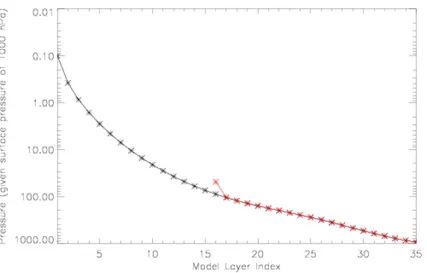
IGCM4 exists in three standard configurations: a spectral truncation of T42, equivalent to a horizontal gridpoint resolution of approximately 2.8◦ _{and 20 layers in the vertical,}

denoted T42L20, which is the standard configuration for studies of the troposphere and climate; T42L35, which enables study of the stratosphere on climate; T170L20,

10

which enables study of mesoscale phenomena such as weather fronts and tropical waves. The L20 and L35 configurations reach from the surface to 50 hPa and 0.1 hPa respectively, and are shown in Fig. 1. The lowest 19 model layers in each configura-tion have exactly the same values, so that only the stratosphere is di_fferent, enabling more traceability when comparing different model configurations. The model has been

15

parallelised using MPI and has been tested on two systems, the UK Universities High Performance system HECToR, and the University of East Anglia’s High Performance Cluster.

2.2 Parallelisation

The spectral code is parallelised using a so-called 2-D decomposition (Foster and

Wor-20

ley, 1997; Kanamitsu et al., 2005). In a 2-D decomposition, two of the three dimensions are divided across the processors, and so there is a column and row of processors, with the columns divided across one dimension and the rows across another. Com-pared with a 1-D decomposition, a 2-D decomposition increases the number of trans-positions that need to be made to go from spectral-space to grid-space and back again.

(5)

GMDD

7, 5517–5545, 2014

M. Joshi et al.

Title Page

Tables Figures

◭ ◮

Back Close

Full Screen / Esc

Discussion

P

a

per

|

Discus

sion

P

a

per

|

Discussion

P

a

per

|

Discussion

P

a

per

|

However the advantage is that each transposition is only amongst processor elements (henceforth PEs) either on the same column or the same row. Any transposition for 1-D decomposition requires all the PEs to communicate with one another, which increases the size of buffers passed between PEs, communication latency, and slows down the model. Han and Juang (2004) found that a 2-D decomposition is about twice as fast as

5

a 1-D decomposition.

More details of the different IGCM configurations are given here: http://www.met.reading.ac.uk/~mike/dyn_models/igcm/

http://www.met.rdg.ac.uk/~lem/large_models/igcm/

http://www.met.reading.ac.uk/~lem/large_models/igcm/parallel/.

10

The model’s performance on the UEA cluster is as follows: T42L35: ∼75 model

years day−1 _{on 32 processors); T42L20:}

∼200 model years day−1 on 32 processors;

T170L20_∼29 model months day−1_{on 64 processors.}

2.3 Surface and boundary layer processes and atmospheric physics

Over land, each grid point has a land-surface type based on present-day

observa-15

tions: there are 8 types (ice, inland water, forest, grassland, agriculture, tundra, swamp, desert). Each land-surface type has its own value for snow-free albedo A, snow-covered albedoS, the height at which total albedo reaches (A+S)/2, and roughness length.

Whenever snowmelt occurs in the model, the snowmelt moistens soil so that the soil

20

water is 2/3 of the saturated value. This is a very simple parameterisation of snowmelt percolating through soil and helps to alleviate warm biases in late spring and summer in Eastern Eurasia, consistent with more complex GCMs such as e.g. HadGEM2.

A maximum effective depth for snow of 15 m exists to prevent slow drifts in heat capacity and hence temperature and energy balance, since there is no physics in the

25

(6)

GMDD

7, 5517–5545, 2014

M. Joshi et al.

Title Page

Tables Figures

◭ ◮

Back Close

Full Screen / Esc

Discussion

P

a

per

|

Discus

sion

P

a

per

|

Discussion

P

a

per

|

Discussion

P

a

per

|

slowly eroding away snow cover over decades. At present, these fixed land-ice points are set to be Antarctica and Greenland.

The effect of sea-ice in IGCM is implemented by assuming a linear change from 0 to

−2◦C in these surface properties: roughness, albedo and heat capacity. This replaces

the sudden change of surface properties at ₋2◦_{C, which is unrealistic given partial} 5

ice cover in most oceans, and also removes a bias in that while sea-ice forms from saline water at−2◦C, it melts at 0◦C, since ice is mostly composed of fresh water. A

combination of ice and open water is therefore desirable between₋2 and 0◦_C.

The amount that surface heat fluxes can be amplified by convectively unstable con-ditions above their values at neutral or zero stability has been limited to 4.0. This value

10

has been chosen to limit latent heat fluxes over the ocean and sensible heat fluxes over the land to better match observations, although it is still a simplification of more complex schemes that involve the Richardson number (e.g. Louis, 1979), since it is entirely stability-based.

2.4 Tropospheric radiation and clouds

15

The NIKOSRAD radiation scheme in IGCM3 (Forster et al., 2000) has been replaced with a modified version of the Morcrette radiation scheme (Zhong and Haigh, 1995) which originally written for the ECMWF model. A transitional version of IGCM3, called IGCM3.1, has existed with this radiation scheme for some time, and many climatic (e.g. Bell et al., 2009; Cnossen et al., 2011) and climate-chemistry (e.g. Highwood

20

and Stevenson, 2003; Taylor and Bourqui, 2005) studies have been conducted with it. The Morcrette radiation scheme has a representation of O₃ absorption of UV be-tween 0.12 and 0.25 µm, 2 visible bands (0.25–0.68 µm, 0.68–4 µm), and 5 infra-red (henceforth IR) bands. Ozone is specified from a zonally averaged climatology of Li and Shine (1995), which is then interpolated to model levels. The solar constant in

25

IGCM4 is 1365 Wm−2, which is more consistent with observations than the older value of 1376 Wm−2_{in IGCM3 and IGCM3.1. The ocean albedo}_A

(7)

GMDD

7, 5517–5545, 2014

M. Joshi et al.

Title Page

Tables Figures

◭ ◮

Back Close

Full Screen / Esc

Discussion

P

a

per

|

Discus

sion

P

a

per

|

Discussion

P

a

per

|

Discussion

P

a

per

|

this manner:

A_o=0.45₋0.30cosϕ. (1) This is a simple parameterisation of the e_ffects of aerosols and solar zenith angle on albedo based on observations so that at the equator A_o=0.15, increasing to 0.3 at 60◦S/N.

5

The clouds have been tuned to better match observations of outgoing infra-red radi-ation and downward surface solar radiradi-ation: the cloud base fraction for deep convective cloud is 4 times the fraction at all other levels, which is consistent with observed convec-tive cloud profiles (Slingo, 1987). Rainout of shallow convecconvec-tive precipitation is allowed over a timescale of 6 h (as opposed to 3 h for deep convection). This rainout helps to

10

slow down the Hadley circulation, whilst removing some of the shallow convective cloud that occurs over subtropical regions.

A version of the Kawai and Inoue (2006) parameterisation for marine stratocumulus cloud has been implemented. This diagnoses low cloud at ocean points depending on the stability of the lowest two model sigma half layers, i.e. between the surface and

15

layer 1, and layer 1 and layer 2, and deposits cloud in the second-to-lowest model layer if diagnosed.

2.5 Stratosphere

A simple gravity wave drag scheme based on Lindzen (1981) had previously been im-plemented in both IGCM1 (Joshi et al., 1995) and IGCM3 (Cnossen et al., 2011). A

20

new scheme calculates drag based on orographic drag, as well as 2 non-orographic modes having horizontal phase speeds of±10 ms−1. The orographic drag source

am-plitude is the magnitude of the zonal wind in the lowest model layer multiplied by the subgrid-scale standard deviation of topography; the non-orographic source amplitude is the magnitude of the zonal wind in the lowest model layer multiplied by a constant

25

(8)

GMDD

7, 5517–5545, 2014

M. Joshi et al.

Title Page

Tables Figures

◭ ◮

Back Close

Full Screen / Esc

Discussion

P

a

per

|

Discus

sion

P

a

per

|

Discussion

P

a

per

|

Discussion

P

a

per

|

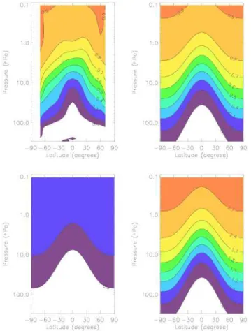
Stratospheric water vapour (henceforth SWV) is calculated by adding a fixed value (3.0_×10−6_{ppmv) onto an amount calculated by a parameterisation that considers}

the stratospheric radiative effects of changing tropospheric methane concentrations. Methane oxidation in the stratosphere depends on the stratospheric chemical envi-ronment and stratospheric residence time. While both the chemical envienvi-ronment and

5

the Brewer-Dobson circulation may change in a changing climate, coupled chemistry-climate model integrations show that their effects on stratospheric methane (and hence on SWV) is small compared to the e_ffect of the changes in methane entering the stratosphere (Eyring et al., 2010), which in turn is given by the change in average tropospheric methane to a good approximation. Hence, the impact of changing

tropo-10

spheric methane can be approximated by calculating the stratospheric distribution of the fraction of oxidised methane, which then is multiplied by the amount of tropospheric methane to give the change in statospheric methane and its contribution to changes in SWV. We define the oxidised fractionβ:

β₍ϕ,z)=1−CH4(ϕ,z)/CH4troposphere (2)

15

wherez is altitude,ϕ is latitude, and any longitudinal variation is assumed to be av-eraged (a very good approximation for the stratosphere). CH₄(ϕ,z) is obtained from satellite measurements by the Halogen Occultation Experiment (HALOE, Russell et al., 1993) over the period 1995–2005. Assuming that two water molecules form for each methane molecule, the water vapour change occurring over a given time interval

20

is given by combining the change in CH₄over the same time interval with the scaling factorβin a similar manner to Fueglistaler and Haynes (2005) giving:

dH₂O(ϕ,z)₌2·β(ϕ,z)·dCH4troposphere (3)

These calculated SWV anomalies are then supplied to the IGCM to allow calculation of the influence of this additional effect on climate. This approach provides excellent

25

(9)

GMDD

7, 5517–5545, 2014

M. Joshi et al.

Title Page

Tables Figures

◭ ◮

Back Close

Full Screen / Esc

Discussion

P

a

per

|

Discus

sion

P

a

per

|

Discussion

P

a

per

|

Discussion

P

a

per

|

Figure 2 (top right) shows an analytical approximation to this distribution, which is then used to calculateβ. The e_ffect is demonstrated by showing the SWV perturbation in ppmv for pre-industrial CH₄ concentrations of 0.75 ppmv (bottom left), and potential future concentrations of CH₄of 2.5 ppmv (bottom right). For reference the background SWV concentration to which this perturbation is added is 3 ppmv.

5

3 Results

3.1 Surface and top-of-atmosphere model climatology

The following results are all from the most commonly used configuration of the IGCM4: sea surface temperature (henceforth SST) is prescribed a monthly-varying climatology (Forster et al., 2000), but land temperature is calculated self-consistently from surface

10

fluxes at each timestep. For this section, the 20-layer T42L20 model has been used, which has been integrated for 50 model years in total.

Figure 3 shows the comparison between NCEP-DOE Reanalysis 2 (Kanamitsu et al., 2002) and IGCM4 surface temperature. During Boreal winter (December–February, or DJF), Fig. 3 (bottom left panel) shows that the model displays a slight cold bias in

15

Northern Eurasia, and a warm bias in the tropical regions and Antarctica. The bias is mostly below 10 K in amplitude, which is good for intermediate models of this type. The boreal summer response (June–August, or JJA) is shown in Fig. 3 (bottom right panel). Here, a warm bias is present over most of the land surface. The warm bias in both summer hemispheres might be partially due to an absence of aerosols in the

20

IGCM: However, even during JJA the magnitude of the bias is less than 10 K almost everywhere, which is reasonable when compared to biases even in CMIP5 models (e.g. Flato et al., 2013, Fig. 9.2).

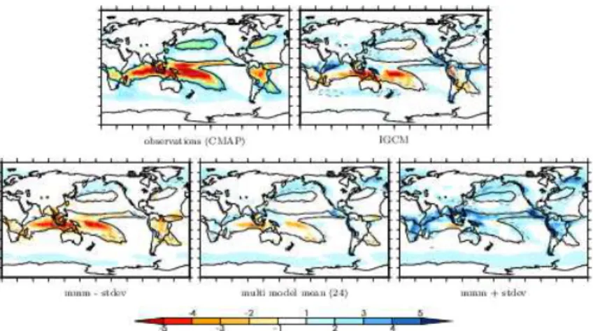
Figure 4 shows the precipitation in DJF in the IGCM (top right panel) compared to the CMAP dataset (Xie and Arkin, 1997) (top left panel). In general the comparison is

25

(10)

con-GMDD

7, 5517–5545, 2014

M. Joshi et al.

Title Page

Tables Figures

◭ ◮

Back Close

Full Screen / Esc

Discussion

P

a

per

|

Discus

sion

P

a

per

|

Discussion

P

a

per

|

Discussion

P

a

per

|

tour in black) being represented quite well. As a guide to the IGCM’s performance in the context of other models, the mean_±one standard deviation precipitation bias amongst a basket of models used in the CMIP5 climate models being used for the UN Inter-governmental Panel on Climate Change’s 5th assessment report (IPCC AR5) is also shown: the comparison is for the CMIP5 model configuration using prescribed “AMIP”

5

SSTs, since coupled ocean-atmosphere biases tend to worsen model performance. The IGCM’s precipitation bias (top right panel) lies within one standard deviation of the AMIP ensemble biases; for instance the dry bias in the Southern Pacific Conver-gence Zone (SPCZ) in the IGCM (top left panel) is 2–5 mm day−1, which is similar in magnitude to the mean minus one standard deviation, suggesting that the IGCM’s

10

performance in this region is within the envelope of state-of-the-art GCMs forced by observed SSTs.

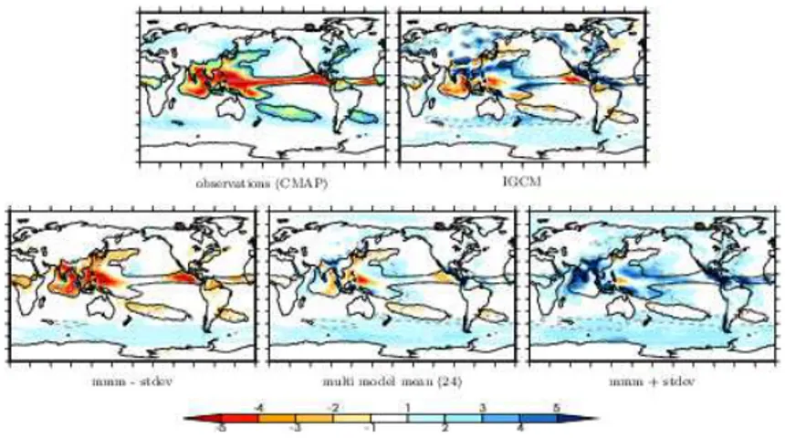
Figure 5 is the same as Fig. 4, but for the JJA period. There are some notable wet biases in IGCM4 (top right panel), particularly in the northern Indian Ocean and Central American regions: however such wet biases are not outside the envelope of the

15

CMIP5 ensemble when comparing the IGCM to the “mean plus one standard deviation” (bottom right panel). This, for the JJA season as with the DJF season, the precipitation bias in IGCM4 is within the range of state-of-the-art GCMs forced by observed SSTs, which provides a good justification for the use of IGCM4 as a simplified climate model. The interaction of precipitation, cloud and radiation, can be studied by examining

20

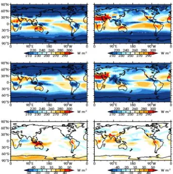
the outgoing long-wave radiation (OLR) field, which is shown in Fig. 6. The bottom left panel shows that the IGCM broadly simulates OLR quite well, with some differences between model and observations in the Maritime continent region. During JJA (bottom right panel), there is a negative bias in OLR over the Indian Ocean, consistent with a slight dry bias there (Fig. 6 bottom right panel). The top-of-atmosphere energy balance

25

in the IGCM is approximately 1–2 Wm−2_{, which is similar to other climate models (e.g.}

(11)

GMDD

7, 5517–5545, 2014

M. Joshi et al.

Title Page

Tables Figures

◭ ◮

Back Close

Full Screen / Esc

Discussion

P

a

per

|

Discus

sion

P

a

per

|

Discussion

P

a

per

|

Discussion

P

a

per

|

3.2 Zonal mean climatology and stratospheric performance

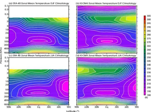
For this section, the 35-layer T42L35 model has been used, which has been integrated for 100 model years in total, in order to average out the effect of stratospheric variability. Figure 7 shows the zonally averaged temperature structure in IGCM4 for the two solsti-tial seasons compared to data from the ERA40 reanalysis (Uppala et al., 2005). During

5

DJF (top panels) the tropical tropopause layer is slightly too cold compared to ERA40. Elsewhere, biases are smaller than 10 K apart from near the summer stratopause, per-haps due to deficiencies in the ozone heating in IGCM4. During JJA, the IGCM4 and ERA40 compare very favourably in their mean temperature structures, being within 10 K almost everywhere, which are comparable errors to other stratospheric models

10

(e.g. Eyring et al., 2006).

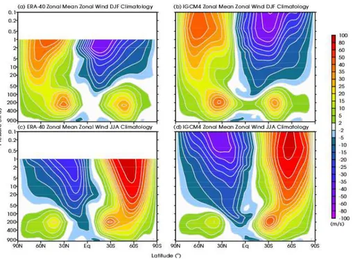
A comparison between the zonally-averaged zonal wind in IGCM4 and ERA40 is shown in Fig. 8, and like Fig. 7, also shows good agreement, perhaps not surprisingly for a field that is expected to be in large-scale thermal balance with temperature. During DJF, the Southern Hemisphere tropospheric jetstream is slightly equatorward of the

15

jet in ERA40, while the Northern Hemisphere’s tropospheric jetstream, is slightly too strong. The winter UTLS region during JJA also displays winds in IGCM4 which are slightly too strong compared to reanalysis. This is probably due to the simplicity of the gravity wave drag scheme.

In both seasons, the strength of the stratospheric jetstreams in IGCM4 compares

20

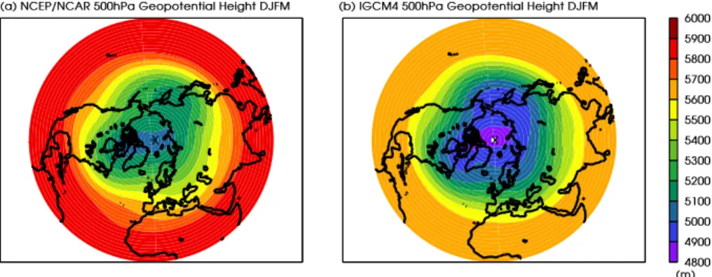
well to ERA40. In northern winter especially this is a sign that the joint effects of gravity wave drag and tropospheric wave forcing in IGCM4 are approximately of the right mag-nitude, since these two factors play a crucial role in controlling the strength of the DJF winter stratospheric jetstream. The zonally asymmetric component of the circulation is apparent from Fig. 9, which shows the geopotential height at 500 hPa. The IGCM4

25

(12)

GMDD

7, 5517–5545, 2014

M. Joshi et al.

Title Page

Tables Figures

◭ ◮

Back Close

Full Screen / Esc

Discussion

P

a

per

|

Discus

sion

P

a

per

|

Discussion

P

a

per

|

Discussion

P

a

per

|

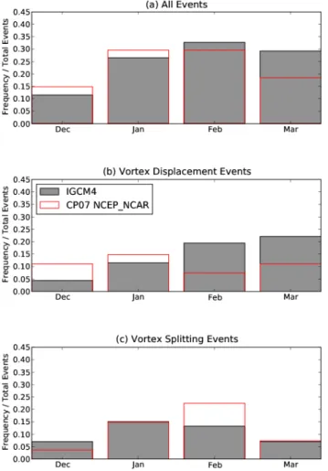
A key issue for stratospheric dynamics and its interplay with tropospheric climate, which is a primary use of this model, is that the stratospheric circulation, and phenom-ena such as sudden stratospheric warmings (henceforth SSWs) are simulated as well as other models. A 200-year long integration of IGCM4 yielded 0.57 SSWs per year as diagnosed by the method of Charlton and Polvani (2007); this should be compared

5

with 0.6 as diagnosed in reanalyses by Charlton and Polvani (2007). 57 % of the SSWs were categorised as “displacement” events using a vortex moment method based on Mitchell et al. (2011), and 43 % diagnosed as “split” events, again broadly consistent with reanalysis output which suggests that just under half of SSWs can be categorised as “split” events (Charlton and Polvani, 2007). The timing of SSWs during boreal winter

10

is shown in Fig. 10. Again, the timings are broadly consistent with reanalysis output, although there are somewhat more displacement events during March than diagnosed from reanalysis.

4 Climate change simulations, discussion and conclusions

When coupled to a slab q flux ocean model, IGCM4 has a climate sensitivity when

15

doubling CO₂from its pre-industrial concentration of 280 ppmv of 2.1 K. This sensitivity is slightly higher than the value of 1.6 K in IGCM3, and is likely due to the changes in cloud physics outlined above. We have not detailed the slab ocean model results because we anticipate that the majority of IGCM4 use as a climate model will be when coupled to a fully dynamic ocean model, as was the case with FORTE. In addition

20

to simulating transient change in a way that a slab ocean models cannot, dynamic ocean models simulate both dynamic and thermodynamic responses, which should both be included to simulate the ocean response to phenomena that cause significant circulation changes in the lower atmosphere (Zhai et al., 2014).

As a first assessment of coupled model performance, the zonally averaged net

sur-25

(13)

GMDD

7, 5517–5545, 2014

M. Joshi et al.

Title Page

Tables Figures

◭ ◮

Back Close

Full Screen / Esc

Discussion

P

a

per

|

Discus

sion

P

a

per

|

Discussion

P

a

per

|

Discussion

P

a

per

|

thermodynamic ocean responses respectively. Figure 11 shows that the broad pat-terns of response are similar in both model and reanalysis. In equatorial regions in-coming solar radiation is not quite balanced by outgoing IR emission because of the presence of tropical convection and thick clouds, leading to positive values (see top panel); the intense rainfall associated with such convection is shown in the top

pan-5

els of Figs. 4 and 5. In subtropical regions, a lack of cloud leads to more IR emission and negative values in both reanalysis and IGCM4. The pattern of wind stress curl (see bottom panel) is indicative of the combined effects of midlatitude westerlies, and subtropical and tropical trade winds, and is similar in both model and reanalysis apart from the southern ocean westerlies being slightly too equatorward in the model, and

10

the Arctic, where the IGCM fails to reproduce large values associated with mesoscale circulations (e.g. Condron and Renfrew, 2013) that the model cannot represent given its horizontal resolution.

Aerosols are not in the standard IGCM4: their effect on surface temperatures have been parameterised by slightly raising the albedo of land and ocean. This is because

15

even CMIP5 GCMs have trouble accurately representing the forcing due to di_fferent types of aerosol. In addition, even the aerosol in the IGCM only deals with the direct ef-fect, and not the di_fferent indirect e_ffects such as cloud lifetime and particle size that are also present in reality. However, both specific case studies of tropospheric and strato-spheric aerosols have been studied using IGCM3.1 (Highwood and Stevenson, 2003;

20

Ferraro et al., 2014), so future study using IGCM4 remains technically very feasible. To summarise, we have presented the physical details, and major climatological and dynamical features of the IGCM4 climate model. The model provides a fast, paral-lelised alternative to conventional state-of-the-art GCMs, and as such forms part of the “hierarchy of models” used in climate research.

(14)

GMDD

7, 5517–5545, 2014

M. Joshi et al.

Title Page

Tables Figures

◭ ◮

Back Close

Full Screen / Esc

Discussion

P

a

per

|

Discus

sion

P

a

per

|

Discussion

P

a

per

|

Discussion

P

a

per

|

Code availability

The code is available to scientific researchers on request by emailing m.joshi@uea.ac.uk in the first instance. Websites detailing different IGCM con-figurations are given in Sect. 2.2. IGCM4 requires as a prerequisite a fortran compiler, the nupdate code management utility, and MPI routines for parallel integrations

5

(although IGCM4 is designed to run on one processor).

Acknowledgements. Model simulations were carried out on the High Performance Computing Cluster supported by the Research and Specialist Computing Support service at the Univer-sity of East Anglia. AOC acknowledges the support of the UK Natural Environment Research Council (NERC). CMAP Precipitation data provided by the NOAA/OAR/ESRL PSD, Boulder,

10

Colorado, USA, from their Web site at http://www.esrl.noaa.gov/psd/. We acknowledge the as-sistance of M. Blackburn, D. Stevens, B. Sinha, A. Blaker, A. Ferraro, E. Highwood, K. Shine, and C. Bell.

References

Bell, C., Gray, L. J., Charlton-Perez, A., Joshi, M. M., and Scaife, A.: Stratospheric

Communi-15

cation of El Niño Teleconnections to European Winter, J. Climate, 22, 4083–4096, 2009. Taylor, C. P. and Bourqui, M. B.: A new fast stratospheric ozone chemistry scheme in an

inter-mediate general-circulation model. I: Description and evaluation, Q. J. Roy. Meteorol. Soc., 131, 2225–2242, 2005.

Charlton, A. J. and Polvani, L. M.: A new look at stratospheric sudden warmings. Part I:

Clima-20

tology and modeling benchmarks, J. Climate, 20, 449–469, 2007.

Cnossen, I., Lu, H., Bell, C. J., Gray, L. J, and Joshi, M. M.: Solar signal propagation: The role of gravity waves and stratospheric sudden warmings, J. Geophys. Res., 116, D02118, doi:10.1029/2010JD014535, 2011.

Collins, M. and James, I. N.: Regular baroclinic transient waves in a simplified global circulation

25

model of the Martian atmosphere, J. Geophys. Res., 100, 14421–14432, 1995.

(15)

GMDD

7, 5517–5545, 2014

M. Joshi et al.

Title Page

Tables Figures

◭ ◮

Back Close

Full Screen / Esc

Discussion

P

a

per

|

Discus

sion

P

a

per

|

Discussion

P

a

per

|

Discussion

P

a

per

|

Eyring, V., Butchart, N., Waugh, D. W., Akiyoshi, H., Austin, J., Bekki, S., Bodeker, G. E., Boville, B. A., Brühl, C., Chipperfield, M. P., Cordero, E., Dameris, M., Deushi, M., Fioletov, V. E., Frith, S. M., Garcia, R. R., Gettelman, A., Giorgetta, M. A., Grewe, V., Jourdain, L., Kinnison, D. E., Mancini, E., Manzini, E., Marchand, M., Marsh, D. R., Nagashima, T., Newman, P. A., Nielsen, J. E., Pawson, S., Pitari, G., Plummer, D. A., Rozanov, E., Schraner, M., Shepherd,

5

T. G., Shibata, K., Stolarski, R. S., Struthers, H., Tian, W., and Yoshiki, M.: Assessment of temperature, trace species, and ozone in chemistry-climate model simulations of the recent past, J. Geophys. Res., 111, D22308, doi:10.1029/2006JD007327, 2006.

SPARC Report on the Evaluation of Chemistry-Climate Models, edited by: Eyring, V., Shepherd, T. G., and Waugh, D. W., SPARC Report No. 5, WCRP-132, WMO/TD-No. 1526, 2010.

10

Cornforth, R. J., Hoskins, B. J., and Thorncroft, C. D.: The impact of moist process on the African easterly jet- African easterly wave system, Q. J. Roy. Meteorol. Soc., 135, 894–913, 2009.

Ferraro, A. J., Highwood, E. J., and Charlton-Perez, A. J., Weakened tropical circulation and reduced precipitation in response to geoengineering, Environ. Res. Lett., 9, 014001

15

doi:10.1088/1748-9326/9/1/014001, 2014.

Flato, G., Marotzke, J., Abiodun, B., Braconnot, P., Chou, S. C., Collins, W., Cox, P., Driouech, F., Emori, S., Eyring, V., Forest, C., Gleckler, P., Guilyardi, E., Jakob, C., Kattsov, V., Reason, C., and Rummukainen, M.: Evaluation of Climate Models, in: Climate Change 2013: The Physical Science Basis. Contribution of Working Group I to the Fifth Assessment Report of

20

the Intergovernmental Panel on Climate Change, edited by: Stocker, T. F., Qin, D., Plattner, G.-K., Tignor, M., Allen, S. K., Boschung, J., Nauels, A., Xia, Y., Bex, V., and Midgley, P. M., Cambridge University Press, Cambridge, United Kingdom and New York, NY, USA, 2013. Foster, I. T. and Worley, P. H.: Parallel Algorithms For The Spectral Transform Method, SIAM

Journal on Scientific Computing, 18, 806–837, doi:10.2172/10168301, 1997.

25

Forster, P. M. De F., Blackburn, M., Glover, R., and Shine, K. P.: An examination of climate sensitivity for idealised climate change experiments in an intermediate general circulation model, Clim. Dynam., 16, 833–849, 2000.

Fueglistaler, S. and Haynes, P. H.: Control of interannual and longer-term variability of strato-spheric water vapor, J. Geophys. Res., 110, D24108, doi:10.1029/2005JD006019, 2005.

30

(16)

GMDD

7, 5517–5545, 2014

M. Joshi et al.

Title Page

Tables Figures

◭ ◮

Back Close

Full Screen / Esc

Discussion

P

a

per

|

Discus

sion

P

a

per

|

Discussion

P

a

per

|

Discussion

P

a

per

|

Highwood, E.-J. and Stevenson, D. S.: Atmospheric impact of the 1783–1784 Laki Erup-tion: Part II Climatic effect of sulphate aerosol, Atmos. Chem. Phys., 3, 1177–1189, doi:10.5194/acp-3-1177-2003, 2003.

Hoskins, B. J. and Simmons, A. J.: A multilayer spectral model and the semi-implicit method, Q. J. Roy. Meteorol. Soc., 101, 637–655, 1975.

5

James, I. N. and Gray, L. J.: Concerning the effect of surface drag on the circulation of a baro-clinic planetary atmosphere, Q. J. Roy. Meteorol. Soc., 114, 619–637, 1986.

Joshi, M. M., Lewis, S. R., Read, P. L., and Catling, D. C.: Western boundary currents in the atmosphere of Mars, Nature, 367, 548–552, 1994.

Joshi, M. M., Lawrence, B. N., and Lewis, S. R.: Gravity wave drag in three-dimensional

atmo-10

spheric models of Mars, J. Geophys. Res., 100, 21235–21245, 1995.

Joshi, M. M., Haberle, R. M., and Reynolds, R. T.: Simulations of the atmospheres of syn-chronously rotating terrestrial planets orbiting M-dwarfs: conditions for atmospheric collapse and implications for habitability, Icarus, 29, 450–465, 1997.

Joshi, M. M., Shine, K. P., Ponater, M., Stuber, N., Sausen, R., and Li, L.: A comparison of

15

climate response to different radiative forcings in three general circulation models: Towards an improved metric of climate change, Clim. Dynam., 20, 843–854, 2003.

Kanamitsu, M., Ebisuzaki, W., Woollen, J., Yang, S.-K., Hnilo, J. J., Fiorino, M., and Potter, G. L.: NCEP-DOE AMIP-II Reanalysis (R-2), Bull. Amer. Meteorol. Soc., 1631–1643, 2002. Kanamitsu, M., Kanamaru, H., Cui, Y., and Juang, H.: Parallel Implementation of the Regional

20

Spectral Atmospheric Model. Scripps Institution of Oceanography, University of California at San Diego, and National Oceanic and Atmospheric Administration for the California Energy Commission, PIER Energy-Related Environmental Research, CEC-500-2005-014, 2005. Kawai, H. and Inoue, T.: A simple parameterisation scheme for subtropical marine

stratocumu-lus, SOLA, 2, 017–020, doi:10.2151/sola.2006-005, 2006.

25

Li, D. and Shine, K. P.: A 4-Dimensional Ozone Climatology for UGAMP Models, UGAMP Inter-nal Report No. 35, April 1995.

Lindzen, R. S.: Turbulence and stress owing to gravity wave and tidal breakdown, J. Geophys. Res., 86, 9707–9714, 1981.

Louis, J. F.: A parametric model of vertical eddy fluxes in the atmosphere, Bound.-Layer Meteor.,

30

(17)

GMDD

7, 5517–5545, 2014

M. Joshi et al.

Title Page

Tables Figures

◭ ◮

Back Close

Full Screen / Esc

Discussion

P

a

per

|

Discus

sion

P

a

per

|

Discussion

P

a

per

|

Discussion

P

a

per

|

Mitchell, D. M., Charlton-Perez, A. J., and Gray, L. J., Characterising the Variability and Ex-tremes of the Stratospheric Polar Vortices Using 2D Moments, J. Atmos. Sci., 1194–1213, 2011.

Rosier, S. M. and Shine, K. P.: The effect of two decades of ozone change on stratospheric temperature as indicated by a general circulation model, Geophys. Res. Lett., 27, 2617–

5

2620, 2000.

Roeckner, E., Brokopf, R., Esch, M., Giorgetta, M., Hagemann, S., Kornblueh, L., Manzini, E., Schlese U., and Schulzweida, U.: Sensitivity of Simulated Climate to Horizontal and Vertical Resolution in the ECHAM5 Atmosphere Model, J. Climate, 19, 3771–3791, 2006.

Russell III, J. M., Gordley, L. L., Park, J. H., Drayson, S. R., Hesketh, W. D., Cicerone, R.

10

J., Tuck, A. F., Frederick, J. E., Harries, J. E., and Crutzen, P. J.: The Halogen Occultation Experiment, J. Geophys. Res., 98, 10777–10798, 1993.

Sinha, B., Hirschi, J., Bonham, S., Brand, M., Josey, S. A., Smith, R., and Marotzke, J.: Mountain ranges favour vigorous Atlantic Thermohaline Circulation, Geophys. Res. Lett., 39. L02705, doi:10.1029/2011GL050485, 2012.

15

Slingo, J. M.: The development and verification of a cloud prediction scheme for the ECMWF model, Q. J. Roy. Meteorol. Soc., 113, 899–927, 1987.

Thorncroft, C. D., Hoskins, B. J., and McIntyre, M. E.: Two paradigms of baroclinic lifecycle behaviour, Q. J. Roy. Meteorol. Soc., 119, 17–55, 1993.

Valdes, P. J. and Hoskins, B. J.: Nonlinear Orographically Forced Planetary Waves, J. Atmos.

20

Sci., 48, 2089–2106, 1991.

Uppala, S. M., Kållberg, P. W., Simmons, A. J., Andrae, U., da Costa Bechtold, V., Fiorino, M., Gibson, J. K., Haseler, J., Hernandez, A., Kelly, G. A., Li, X., Onogi, K., Saarinen, S., Sokka, N., Allan, R. P., Andersson, E., Arpe, K., Balmaseda, M. A., Beljaars, A. C. M., van de Berg, L., Bidlot, J., Bormann, N., Caires, S., Chevallier, F., Dethof, A., Dragosavac, M.,

25

Fisher, M., Fuentes, M., Hagemann, S., Hólm, E., Hoskins, B. J., Isaksen, L., Janssen, P. A. E. M., Jenne, R., McNally, A. P., Mahfouf, J. F., Morcrette, J. J., Rayner, N. A., Saunders, R. W., Simon, P., Sterl, A., Trenberth, K. E., Untch, A., Vasiljevic, D., Viterbo, P., and Woollen, J.: The ERA-40 re-analysis, Q. J. Roy. Meteorol. Soc., 131, 2961–3012, 2005.

Xie, P. and Arkin, P. A.: Global precipitation: a 17-year monthly analysis based on gauge

ob-30

(18)

GMDD

7, 5517–5545, 2014

M. Joshi et al.

Title Page

Tables Figures

◭ ◮

Back Close

Full Screen / Esc

Discussion

P

a

per

|

Discus

sion

P

a

per

|

Discussion

P

a

per

|

Discussion

P

a

per

|

Zhai, X., Johnson, H. L., and Marshall, D. P.: A simple model of the response of the Atlantic to the North Atlantic Oscillation, J. Climate, 27, 4052–4069, doi:10.1175/JCLI-D-13-00330.1, 2014.

Zhong, W. Y. and Haigh, J. D.: Improved broad-band emissivity parameterization for water vapor cooling calculations, J. Atmos. Sci., 52, 124–138, 1995.

(19)

GMDD

7, 5517–5545, 2014

M. Joshi et al.

Title Page

Tables Figures

◭ ◮

Back Close

Full Screen / Esc

Discussion

P

a

per

|

Discus

sion

P

a

per

|

Discussion

P

a

per

|

Discussion

P

a

per

|

(20)

GMDD

7, 5517–5545, 2014

M. Joshi et al.

Title Page

Tables Figures

◭ ◮

Back Close

Full Screen / Esc

Discussion

P

a

per

|

Discus

sion

P

a

per

|

Discussion

P

a

per

|

Discussion

P

a

per

|

Figure 2.The fraction of oxidised methane (which is linked to CH4 concentration, see Eq. 1)

derived from HALOE data (top left panel); the analytical approximation which extends to the poles (top right panel); the perturbation to stratospheric water vapour (SWV) (ppmv) in pre-industrial conditions, when CH4 is 0.75 ppmv (bottom left); the perturbation to SWV (ppmv) if

(21)

GMDD

7, 5517–5545, 2014

M. Joshi et al.

Title Page

Tables Figures

◭ ◮

Back Close

Full Screen / Esc

Discussion

P

a

per

|

Discus

sion

P

a

per

|

Discussion

P

a

per

|

Discussion

P

a

per

|

Figure 3.Surface temperature (◦_{C) in IGCM4 (top panels), observations (middle panels) and}

(22)

GMDD

7, 5517–5545, 2014

M. Joshi et al.

Title Page

Tables Figures

◭ ◮

Back Close

Full Screen / Esc

Discussion

P

a

per

|

Discus

sion

P

a

per

|

Discussion

P

a

per

|

Discussion

P

a

per

|

Figure 4. Observed precipitation (mm day−1

(23)

GMDD

7, 5517–5545, 2014

M. Joshi et al.

Title Page

Tables Figures

◭ ◮

Back Close

Full Screen / Esc

Discussion

P

a

per

|

Discus

sion

P

a

per

|

Discussion

P

a

per

|

Discussion

P

a

per

|

(24)

GMDD

7, 5517–5545, 2014

M. Joshi et al.

Title Page

Tables Figures

◭ ◮

Back Close

Full Screen / Esc

Discussion

P

a

per

|

Discus

sion

P

a

per

|

Discussion

P

a

per

|

Discussion

P

a

per

|

(25)

GMDD

7, 5517–5545, 2014

M. Joshi et al.

Title Page

Tables Figures

◭ ◮

Back Close

Full Screen / Esc

Discussion

P

a

per

|

Discus

sion

P

a

per

|

Discussion

P

a

per

|

Discussion

P

a

per

|

(26)

GMDD

7, 5517–5545, 2014

M. Joshi et al.

Title Page

Tables Figures

◭ ◮

Back Close

Full Screen / Esc

Discussion

P

a

per

|

Discus

sion

P

a

per

|

Discussion

P

a

per

|

Discussion

P

a

per

|

(27)

GMDD

7, 5517–5545, 2014

M. Joshi et al.

Title Page

Tables Figures

◭ ◮

Back Close

Full Screen / Esc

Discussion

P

a

per

|

Discus

sion

P

a

per

|

Discussion

P

a

per

|

Discussion

P

a

per

|

(28)

GMDD

7, 5517–5545, 2014

M. Joshi et al.

Title Page

Tables Figures

◭ ◮

Back Close

Full Screen / Esc

Discussion

P

a

per

|

Discus

sion

P

a

per

|

Discussion

P

a

per

|

Discussion

P

a

per

|

(29)

GMDD

7, 5517–5545, 2014

M. Joshi et al.

Title Page

Tables Figures

◭ ◮

Back Close

Full Screen / Esc

Discussion

P

a

per

|

Discus

sion

P

a

per

|

Discussion

P

a

per

|

Discussion

P

a

per

|