A STREAMFLOW FORECASTING FRAMEWORK USING
MULTIPLE CLIMATE AND HYDROLOGICAL MODELS
1Paul J. Block, Francisco Assis Souza Filho, Liqiang Sun, and Hyun-Han Kwon2
ABSTRACT: Water resources planning and management efficacy is subject to capturing inherent uncertainties stemming from climatic and hydrological inputs and models. Streamflow forecasts, critical in reservoir operation and water allocation decision making, fundamentally contain uncertainties arising from assumed initial condi-tions, model structure, and modeled processes. Accounting for these propagating uncertainties remains a formi-dable challenge. Recent enhancements in climate forecasting skill and hydrological modeling serve as an impetus for further pursuing models and model combinations capable of delivering improved streamflow fore-casts. However, little consideration has been given to methodologies that include coupling both multiple climate and multiple hydrological models, increasing the pool of streamflow forecast ensemble members and accounting for cumulative sources of uncertainty. The framework presented here proposes integration and offline coupling of global climate models (GCMs), multiple regional climate models, and numerous water balance models to improve streamflow forecasting through generation of ensemble forecasts. For demonstration purposes, the framework is imposed on the Jaguaribe basin in northeastern Brazil for a hindcast of 1974-1996 monthly streamflow. The ECHAM 4.5 and the NCEP⁄MRF9 GCMs and regional models, including dynamical and statis-tical models, are integrated with the ABCD and Soil Moisture Accounting Procedure water balance models. Pre-cipitation hindcasts from the GCMs are downscaled via the regional models and fed into the water balance models, producing streamflow hindcasts. Multi-model ensemble combination techniques include pooling, linear regression weighting, and a kernel density estimator to evaluate streamflow hindcasts; the latter technique exhibits superior skill compared with any single coupled model ensemble hindcast.
(KEY TERMS: surface water hydrology; precipitation; computational methods; streamflow; forecast; uncertainty; multi-model; ensemble; Brazil.)
Block, Paul J., Francisco Assis Souza Filho, Liqiang Sun, and Hyun-Han Kwon, 2009. A Streamflow Forecasting Framework Using Multiple Climate and Hydrological Models.Journal of the American Water Resources Associa-tion(JAWRA) 45(4):828-843. DOI: 10.1111⁄j.1752-1688.2009.00327.x
INTRODUCTION
Water resources planning and management effi-cacy is subject to capturing inherent uncertainties
stemming from climatic and hydrological inputs and models. Streamflow forecasts, critical in reservoir operation and water allocation decision making, fun-damentally contain uncertainties arising from assumed initial conditions, model structure, and
1Paper No. JAWRA-08-0075-P of theJournal of the American Water Resources Association(JAWRA). Received April 22, 2008; accepted December 17, 2008.ª2009 American Water Resources Association.Discussions are open until six months from print publication.
2Respectively Associate Research Scientist, Research Scientist (Block, Sun), International Research Institute for Climate and Society (IRI), Columbia University, Lamont Campus, 61 Route 9W, Monell Building, Palisades, New York 10964; Professor (Souza Filho), Federal University of Ceara´, Fortaleza, Brazil; and Senior Researcher (Kwon), Korea Institute of Construction Technology, Goyang-Si, Korea (E-Mail⁄Block: [email protected]).
modeled processes (Georgakakos et al., 2004; Doblas-Reyes et al., 2005). Accounting for these propagating uncertainties remains a formidable challenge.
Approaches to streamflow forecasting predomi-nantly fall into two categories: statistical or dynami-cal (climatic-hydrologidynami-cal model integration). The former frequently utilizes predictors of sea-surface temperature or a related index to directly estimate streamflow through statistical techniques (Souza Fil-ho and Lall, 2003). The second approach seeks to cou-ple climate and hydrological processes by passing downscaled information in an iterative (online) or sta-tic (offline) fashion. Although the mechanics differ, accounting for forecast uncertainty is achievable in either approach by applying Monte Carlo or stochas-tic methodologies to generate forecast ensembles. Recent enhancements in climate forecasting skill and hydrological modeling serve as an impetus for further pursuing models capable of delivering improved streamflow forecasts (Cane et al., 1986; Barnston
et al., 1999a,b; Mason et al., 1999; Landman et al., 2001; Rajagopalan et al., 2002).
Significant attention has been given lately to incorporation of multiple climate models or multiple hydrological models for forecasting climatic or hydro-logical variables (Krishnamurti et al., 1999, 2000; Doblas-Reyes et al., 2000; Hagedorn, 2001; Kumar
et al., 2001; Robertson et al., 2004; Hagedorn et al., 2005; Tebaldi et al., 2005; Block and Rajagopalan, 2008; Chowdhury and Sharma, 2008; Devineni
et al., 2008; Mujumdar and Ghosh, 2008). Previous research supports the notion that combinations of model forecasts may produce more robust forecast skill and reliability than single model forecasts, attributable to inclusion of varying initial conditions and processes (Beven and Freer, 2001; Georgakakos
et al., 2004; Doblas-Reyes et al., 2005; Regonda
et al., 2006). Numerous multi-model ensemble combi-nation techniques have been developed, demonstrat-ing improved streamflow forecast skill (Rajagopalan
et al., 2002; Doblas-Reyes et al., 2005; Yun et al., 2005; Ajami et al., 2006; Duan et al., 2006). Little consideration, however, has been given to methodol-ogies that include dynamical coupling of both multi-ple climate and multiple hydrological models, further increasing the pool of streamflow forecast ensemble members and accounting for cumulative sources of uncertainty. This approach, presented here, creates a robust, inclusive system, demonstrat-ing various options available for improved stream-flow forecasting.
In this paper, a general streamflow forecasting framework incorporating multiple climate and hydro-logic models from dynamical and statistical approaches is proposed. The Problem Setting, includ-ing descriptions of existing climate, hydrologic
and coupled model systems, and processes is initially outlined. Following is a Description of the Application Site Chosen and Associated Datasets employed for demonstration. The proposed forecasting framework is subsequently outlined in detail, followed by Results of imposing this framework through a hindcast on the application site. The paper concludes with a Sum-mary and Discussion.
PROBLEM SETTING
Perfect forecast models in climate and hydrology are nonexistent. For improved skill, risk assess-ment, and probabilistic interpretation, forecasts must be placed in a context based on inherent and cumulative uncertainty created throughout the mod-eling process. Climate models suffer from assump-tions of initial and boundary condiassump-tions; dynamical hydrological (i.e., rainfall-runoff) models lack in pro-cess description and resolution, parameter estima-tion, and model structure (Stern and Miyakoda, 1995; Goddard et al., 2001; Georgakakos et al., 2004; Doblas-Reyes et al., 2005; Kang and Yoo, 2006).
Global climate models (GCMs) are based on the general principles of fluid dynamics and thermody-namics. Other processes, such as convection, occur-ring on scales too small to be resolved directly, require parameterization. GCMs are typically run at relatively coarse spatial resolutions, generally greater than 2.0 latitudinally and longitudinally. The direct result of the poor spatial resolution pro-duces a serious spatial scale mismatch between the available climate forecasts and the scale of interest to most climate forecast users. To overcome this, sta-tistical or dynamical regional climate models (RCMs), with a higher spatial resolution, are constructed for limited areas. Relatively high-resolution RCMs, dri-ven by low resolution GCMs, can provide meaningful small-scale features over a limited region at afford-able computational cost compared with high-resolu-tion GCMs.
some routing of streamflow between grid boxes (Aj-ami et al., 2006). Although distributed models are considered more complex than lumped models, they have not definitively shown their superiority in terms of streamflow forecast skill (Reed et al., 2004) and continue to suffer from inherent problems (Beven, 2001).
Coupling climate and dynamical hydrologic mod-els to function in combination may occur through either an online or offline process. Online processes allow feedback between models in an iterative approach, and typically require the hydrological models to be distributed such that the grid box size is equivalent to the climate model grid box size. Offline coupled models, however, operate in a con-secutive manner; the climate model completes its simulation before passing climatic values to the hydrological model. Hydrological models may there-fore be of either a lumped or distributed nature. The framework outlined in this work adopts an off-line approach.
As previously stated, ensemble forecasting is becoming increasingly popular (Tracton and Kalnay, 1993; Harrisonet al., 1995; Doblas-Reyes et al., 2000, 2005; Fritsch et al., 2000; Palmer et al., 2000, 2004). Combining forecasts (from single or multiple models) initialized with differing conditions or assumptions often better predicts the forecast probability density function and has been shown to generally provide superior overall skill (Doblas-Reyes et al., 2005). Additionally, inclusion of forecasts from multiple models may better account for uncertainties in physi-cal processes and model structure (Georgakakos
et al., 2004). The driving motivation for this research is to create a framework in which the advantages of including multiple models may be exploited at several stages of the process.
Various techniques exist for combining forecasts from multiple predictions, however applications in a hydrologic context have only been applied in the rela-tively recent past (McLeod et al., 1987; Shamseldin and O’Connor, 1999; Ajami et al., 2006). The simplest approach is to equally weight all forecasts and pool them together (Barnstonet al., 2003; Robertsonet al., 2004; Hagedorn et al., 2005). Optimally weighted models based on historical performance advances this methodology. More sophisticated combination tech-niques include regression and Bayesian approaches (Rafteryet al., 1997; Rajagopalanet al., 2002; Doblas-Reyeset al., 2005; Marshallet al., 2005; Ajamiet al., 2006; DelSole, 2006). Ensemble means do not necessi-tate superior forecasts in comparison with single model predictions; however, the clear advantage of ensemble forecasting is apparent in a probabilistic framework (Palmer et al., 2004; Doblas-Reyes et al., 2005).
DESCRIPTION OF APPLICATION SITE AND DATA
Iguatu Basin in the Jaguaribe River Basin, Brazil
The streamflow forecasting framework proposed, and outlined in the subsequent section, is applied to the Iguatu basin (19,100 km2), which lies within the larger Jaguaribe basin, a 72,000 km2semiarid area in northeast Brazil. The city of Iguatu lies at the outlet of this basin on the Jaguaribe River. The basin experi-ences one rainy season annually, from January to May. During this time, the Atlantic Intertropical Con-vergence Zone (ITCZ) reaches its southernmost posi-tion, lying very near to or over the region, enhancing atmospheric instability and producing precipitous sys-tems. Abnormal latitudinal migrations of the ITCZ are associated with excess (southward) or deficit (north-ward) rainfall (Hastenrath and Heller, 1977). Previous investigations have firmly established that sea-surface temperature (SST) anomaly forcing is the primary fac-tor responsible for the interannual variability of rain-fall in northeast Brazil (Moura and Shukla, 1981; Ward and Folland, 1991; Sun et al., 2005). Positive (negative) rainfall anomalies are frequently observed when the Atlantic SSTs are colder (warmer) than nor-mal north of the Equator and warmer (colder) than normal south of the Equator. Droughts also tend to coincide with the El Nin˜o-Southern Oscillation ENSO episodes. Slowly evolving SST anomalies, particularly in the tropical oceans, can be predicted with some degree of skill at lead times of several months (Zebiak and Cane, 1987). Seasonal rainfall forecasts (February to May) issued in January are skillful over northeast Brazil (Sun et al., 2006). Since 2001, an operational regional climate forecast has been maintained by the climate and water foundation for the State of Ceara´ (FUNCEME) and the International Research Institute for Climate and Society (IRI). Offline coupling of an RCM and the Soil Moisture Accounting Procedure (SMAP) hydrologic model was developed by Souza Filho and Porto (2003).
Application Site Data
ECHAM4.5 and NCEP⁄MRF9 GCM precipitation data is obtained from the IRI Data Library and based on observed SSTs and 10 ensemble members each (Kumar et al., 1996; Livezey et al., 1996; Roeckner
et al., 1996; Saha et al., 2006).
FORECASTING APPROACH AND MODEL DESCRIPTIONS
This approach proposes the integration of multiple GCMs, RCMs, hydrologic models, and multi-model combination techniques in successive fashion for ensemble streamflow forecasting. The overall frame-work proposed is presented pictorially in Figure 2. Generally, persisted or forecasted sea-surface temper-atures drive GCMs, producing low resolution precipi-tation that may be downscaled with statistical or dynamical RCMs. Dynamical approaches often require bias correction based on hindcasts and histor-ical observations. If desired, downscaled precipitation (and other climatic variables) may be run through a weather generator to produce an ensemble of plausi-ble scenarios, further increasing the forecast pool. Downscaled precipitation is fed into hydrological models to generate streamflow forecasts, which are subsequently weighted and combined, as a final step, to create a multi-model ensemble for probabilistic evaluation. To demonstrate the framework on the Ig-uatu basin, a streamflow hindcast is performed over the 1974-1996 period. The following sections describe
specific models chosen for analysis, and by no means constitute the full array of possibilities available in the proposed framework.
Climate Models
Global Climate Models. The atmospheric GCMs chosen for framework demonstration are the
ECHAM4.5, as developed at the Max Plank
Institute for Meteorology in Germany (Roeckner
et al., 1996), and the NCEP⁄MRF9, developed by
FIGURE 1. January to June Streamflow on the Jaguaribe River at Iguatu, Brazil, for 1912-1996.
the U.S. National Weather Service’s National Cen-ters for Environmental Prediction (Kumar et al., 1996; Livezey et al., 1996; Saha et al., 2006). For this hindcast demonstration, each model is run in simulation mode, driven by concurrent SSTs. Alter-natively, a retrospective format could be evaluated, such that forecasted or persisted SSTs replace observed SSTs.
Regional Climate Model. Dynamical:Regional Spectral Model. The NCEP RSM (Juang and Kanami-tsu, 1994; Juang et al., 1997) is selected for dynami-cal downsdynami-caling. An ensemble of 10 runs with the nested NCEP RSM – ECHAM4.5 AGCM system, using observed SSTs, is created for the period of Jan-uary to June 1971-2000. For further model details, including coupling with the ECHAM4.5 GCM, please contact the authors. Dynamical downscaling models utilizing the NCEP⁄MRF9 GCM are not yet available; additional RCMs over northeast Brazil are currently under development.
Statistical:Linear Regression With Principal Components. Statistical downscaling of climatic vari-ables from the GCMs offers an alternative approach to dynamical downscaling, and is traditionally significantly simpler in nature (Wilby et al., 1998; Murphy, 1999; Landman et al., 2001). The methodol-ogy adopted for downscaling of precipitation utilizes a cross-validated linear regression model with princi-pal components (PCs) of the GCM forecasted precipi-tation ensemble mean acting as predictors. The spatial domain included is identical to that employed by the Regional Spectral Model (RSM) Principal component analysis, widely used in climate research, decomposes a space-time random field into orthogo-nal space [Eigenvector (E)] and time (PC) patterns using Eigen decomposition (Von Storch and Zwiers, 1999). The patterns are ordered according to the percentage of variance captured. This analysis technique additionally eliminates multicollinearities and limits unstable or unreasonable estimates of weights. The precipitation downscaling methodology, outlined in the following algorithm, is repeated for each month (six) from each GCM for January to June, 1971-1996:
(1) Model PCs are based on the 1950-1996 GCM monthly precipitation ensemble mean, X, and constructed with the following relationship:
PCT¼ETXT ð1Þ
The first n PCs, explaining the majority of the variance, are retained and form the suite of model predictors.
(2) Regression coefficients, b0,…, bn, based on the ensemble mean, are identified through a least squares linear regression model. The following equation creates a best fit estimate by optimally weighting model PCs to minimize errors.
OBSt ¼b0þb1PC1;tþb2PC2;tþ:::þ
bnPCn;tþet t¼1tot;
ð2Þ
where OBS is the observed precipitation value at time t, t* is the number of time periods (years), and e corresponds to model residuals.
(3) PCs for the prediction month, PCP, (individual ensemble member) are acquired using the eigenvectors developed in step (1) and applying Equation (1) with X representing the GCM prediction month hindcast.
(4) Retaining the regression coefficients from Equa-tion (2), the predicEqua-tion month PCs are applied to the following equation to determine the monthly precipitation hindcast,H.
Ht¼b0þb1PCP1;tþb2PCP2;tþ::: þ
bnPCPn;
t¼1to t ð3Þ
Equation (3) is utilized for each of the 10 ensemble members corresponding to the specified month and GCM.
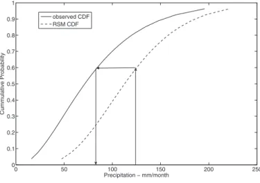
Bias Correction: Probability Mapping. Dynam-ical or physDynam-ically based model outputs typDynam-ically con-tain some systematic bias and require correction, unlike statistical models which inherently account for biases by their empirical nature. Probability mapping is selected here for bias correction of the monthly RSM precipitation data (averaged over the 12 RSM grid boxes), and is based on two cumula-tive distribution functions (CDF): (1) the historical observed data, and (2) all RSM ensemble data pooled by months (akin to Ines and Hansen, 2006). The latter CDF is created by combining all hind-casts for a given month using all ensemble mem-bers. Each CDF is fit with a gamma distribution, saving the shape and scale parameters. A given monthly RSM precipitation value from a hindcast
ensemble member is then bias corrected by
Hydrological Models
A plethora of lumped and distributed hydrological models have been developed over the past decades, providing a wide array of choices. Two rainfall-runoff models are selected for inclusion in this work: the ABCD model, well recognized and accepted in the hydrology community (Thomas, 1981; Thomas et al., 1983) and the SMAP applied to various basins within Brazil (Lopeset al., 1982; Lopes and Porto, 1993). The models are both run at monthly time-steps, effectively relegating them to water balance models. Models requiring higher temporal resolution may alterna-tively be selected, dependent on forecasting needs.
SMAP is a conceptual, lumped model containing two reservoirs (subsurface and ground water) and four parameters: soil saturation capacity, surface flow, a recharge coefficient, and a base flow recession coefficient. The rainfall-runoff component is founded on the Soil Conservation Service equation and utilizes basin average precipitation and evapotranspiration.
ABCD is a nonlinear watershed model, which repre-sents soil moisture storage, ground water storage, direct runoff, ground water outflow to the stream chan-nel, and actual evapotranspiration. Inputs include pre-cipitation and potential evapotranspiration. Its performance in comparison with other monthly water balance models has lead to its recommended use (Alley, 1984, 1985; Vandewieleet al., 1992).
Multi-Model Hindcast Ensemble Combinations and Skill Scores
Three techniques for combining hindcast ensembles from multiple models are selected to demonstrate
various levels of sophistication. Monthly streamflow hindcasts (January to June) from the hydrological models are aggregated to seasonal totals prior to com-bination. Aggregating temporally tends to smooth the data and increase skill by reducing the noisy month-to-month variability. Seasonal totals are also of particular interest for the application site in regards to agriculture and water resources infrastructure planning.
The most straightforward technique for combining ensembles is pooling, in which all ensemble members are given equal weight and joined into a single multi-model ensemble (Barnston et al., 2003; Robertson
et al., 2004; Hagedorn et al., 2005). Basic statistics (median, standard deviation, etc.) are easily com-puted. It has been shown that even this simple approach typically proves superior to a single forecast due to its higher reliability (Doblas-Reyeset al., 2005; Hagedornet al., 2005).
The second methodology utilizes a least squares lin-ear regression technique, of which a form has been used for some time by NCEP for seasonal climate fore-casts (Van den Dool, March 27, 2008, IRI Seminar Ser-ies). The particular version adopted here assigns a weight to model ensembles based on the regression coefficient created by fitting individual ensemble means to observed conditions. Regression coefficients closer to a value of one (similar to observed conditions) are assigned greater proportional weight than coeffi-cients deviating further from one.
The third approach applies a normal kernel den-sity estimator (Bowman and Azzalini, 1997; Bishop, 2006) to calculate the probability density,Pmt, at each hindcast observation from each model using the fol-lowing equation:
Pm;t¼ 1
N X
N
n¼1
1
ffiffiffiffiffiffiffiffiffiffiffiffiffiffi
ð2ph2Þ
p exp
ðxo
;t
xm
;t;nÞ
2
2h2
( )
;
t¼1to t;m¼1to z; ð4Þ
whereN is the total number of ensemble members,h
is the kernel bandwidth, xm,t,n is the hindcast value from model m, in period t, and ensemble member n, and x0,t is the observation in period t (where the probability density is desired). Bandwidth is set as a function of ensemble variance. Optimal weight for each model (wm), constrained between zero and one, is obtained by maximizing the total likelihood (L) over all time periods from all models (Rajagopalan
et al., 2002). For ‘‘z’’ models:
L¼Y
T
t¼1 X
z
m¼1 wmPm
;t
( )
ð5Þ
Skill scores for ensemble hindcast evaluation selected here include median and total root mean square error, Pearson’s correlation coefficients, and rank probability skill score (RPSS) (Wilks, 1995; Sun
et al., 2006; Block and Rajagopalan, 2008). Pearson’s correlation coefficients are calculated using ensemble medians. Relevant equations and descriptions are provided in Appendix I.
RESULTS AND ANALYSIS
Following the framework proposed and models selected, streamflow hindcasts for 1974-1996 at Igua-tu are generated and compared with the observed record. Results at each major stage of the framework are presented.
Climate Model Downscaling
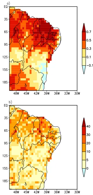
The ability of the nested ECHAM4.5 GCM-RSM model to simulate interannual variability of precipi-tation is illustrated in Figure 4. Temporal anomaly correlation coefficients between observed and simu-lated precipitation ensemble means during the rainy season (Figure 4A) exceed 0.3 (the 90% confi-dence level) over most of northeast Brazil, with a correlation coefficient of 0.72 for the Jaguaribe basin. The strong performance by the model suggests that much of the interannual variability of basin rainfall is associated with global SST variations.
Probabilistic rainfall hindcasts by the nested model provide an estimate of the predictability that may be achievable given a perfect SST forecast. The RPSS for the RSM precipitation ensemble mean averaged over the 30-year hindcast is shown in Figure 4B, and indicates moderate skill (<10%) south of latitude 9 S, but stronger skill (>10%) in northeast Brazil, particu-larly over the basin.
Figure 5 illustrates the raw RSM and observed CDFs required for bias correction of monthly precipi-tation, and clearly indicates a larger bias in the drier January, May, and June months.
The bias correction methodology adopted here is fairly effective for the Jaguaribe basin, yet some years still indicate insufficient or excess precipitation in comparison with the observed record. Figure 6 (top) depicts box plots of the January to June total precipitation for each corrected ensemble member and the observed record for 1971-1996. While for most years the ensemble members envelop the observed value, as desired, a few years indicate
under-or over-predictions by all ensemble members (e.g., 1974 and 1976) even after bias correction, partially attributable to scaling with ensemble means. How-ever, this is expected with ensemble forecasting, and the general wet or dry bias of the RSM model appears to be effectively removed. The correlation coefficient between the dynamically downscaled ensemble mean and observed precipitation over the entire season is 0.82 for the validation period (see Table 1); the median RPSS for the ensemble years equals 0.35, indicating a notable improvement over climatology.
FIGURE 4. Nested ECHAM4.5 GCM-RSM Model Results: (A) Tem-poral Anomaly Correlation Coefficients Between Observed and RSM Ensemble Mean Precipitation, and (B) RPSS for the RSM
FIGURE 5. Cumulative Distribution Functions for 1971-1996 Monthly Precipitation. Solid line represents Iguatu basin observed; dashed lines represent 10 uncorrected RSM ensemble members. Note different scales.
FIGURE 6. Box Plots of Downscaled January to June Total Precipitation Over Iguatu Basin for 1971-1996; Top by Dynamical – Bias Correction, Middle by Statistical – ECHAM4.5, Bottom by Statistical – NCEP⁄MRF9
Statistical downscaling of precipitation from the ECHAM4.5 and NCEP⁄MRF9 GCMs is illustrated similarly in Figure 6 (middle and bottom). Ten PCs are retained for use as predictors in both models, chosen according to scree plot interpretations. These 10 explain approximately 79 and 65% of the vari-ance, respectively (percentages are averages over the 26-year period, or equivalently 26 unique mod-els, as required by the cross-validation methodol-ogy). Associated regression coefficients (excluding b0 – the y-intercept) vary between )2 to +2. General performance is comparable with dynamical down-scaling, with high correlation coefficients (0.88 and 0.85), and robust median RPSS (0.27 and 0.55) for the two models, respectively. The nature of the sta-tistical model allows for the possibility of negative precipitation hindcasts, however the rate of occur-rence is very small (1%); negative values are reset to zero.
The overall high skill scores between the dynami-cal and statistidynami-cal downsdynami-caling models are not sur-prising given ensemble forecasts and temporal aggregation to seasonal values. More interest-ingly, perhaps, is the performance of the two statis-tical downscaling methods, being on par or bettering the complex and computationally demand-ing dynamical method. Retaindemand-ing both methods, however, remains prudent for capturing structural uncertainty.
Hydrological Model Calibration and Validation
The SMAP and ABCD water balance models are calibrated against 1912-1969 monthly streamflow at Iguatu, as indicated in Table 1, by optimizing model parameters. The objective function for optimi-zation in both cases centers on minimizing the sum of the squared errors. Required evapotranspiration values for the calibration period are based on obser-vations. Parameter values for SMAP fell within a reasonable and expected range, with soil saturation
capacity, surface flow, the recharge coefficient, and base flow coefficient equating to 624, 2.7, 0.01, and 0, respectively. ABCD model parameters over the calibration period are 0.98, 284, 0.49, and 0, respec-tively. Parameter value b is high, given its physical interpretation as the upper limit of the sum of evapotranspiration and soil moisture storage, but this phenomenon has been noted by others as well (Thomas et al., 1983; Alley, 1984).
The seasonal time-series (aggregation of January to June) of observed and model produced streamflow during the calibration period are illustrated in Fig-ure 7. Correlation coefficients for both models with observed values are nearly identical at 0.90 and 0.89 for SMAP and ABCD, respectively. The models mimic observed streamflow quite well, with the exception of underestimation in 1924, the wettest year in the cali-bration period. Monthly time-series (not shown here) also indicate strong correlation, with coefficients of approximately 0.87.
Validation of both models is performed over the 1974-1996 period. Evapotranspiration inputs to the model are based on climatological values of the period (to reflect similarity with the coupled model hindcast case). Seasonal correlation coefficients for the SMAP and ABCD models, respectively, are 0.95 and 0.97, indicating very strong model performance according to this metric. In slight contrast to the calibration period performance, both models do remarkably well in estimating high flow seasonal quantities, but are less proficient for low flow sea-sons.
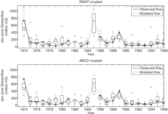
Coupled Climate and Hydrologic Model Hindcast
Coupling the climate and hydrological models, a streamflow hindcast is performed on the 1974-1996 period. Six ensembles of hindcasts (10 members each) are produced by combining the three downscaling techniques with the two hydrological models. Figure 8 portrays results of driving the calibrated SMAP and
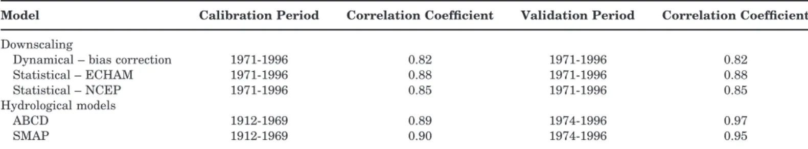
TABLE 1. Calibration and Validation Periods and Correlation Coefficients for Downscaling and Hydrological Models.
Model Calibration Period Correlation Coefficient Validation Period Correlation Coefficient
Downscaling
Dynamical – bias correction 1971-1996 0.82 1971-1996 0.82 Statistical – ECHAM 1971-1996 0.88 1971-1996 0.88
Statistical – NCEP 1971-1996 0.85 1971-1996 0.85
Hydrological models
ABCD 1912-1969 0.89 1974-1996 0.97
SMAP 1912-1969 0.90 1974-1996 0.95
ABCD models with the ECHAM4.5 GCM precipita-tion ensemble dynamically downscaled and bias cor-rected. Figures 9 and 10 are similar excepting that statistical downscaling is employed for the
ECHAM4.5 and NCEP⁄MRF9 GCMs. Streamflow
ensembles are displayed as box plots; observed values are indicated by filled circles. Seasonal time-series of ensemble medians and observed streamflow are
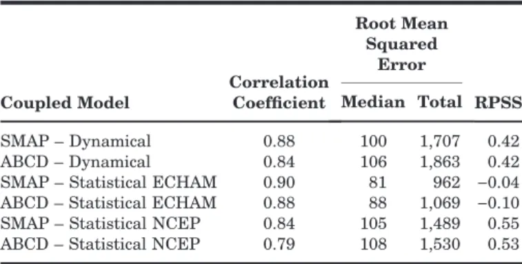
illus-trated by solid and dashed lines, respectively. Notable features include better approximation of 1974 (wet-test year in hindcast period) by the ECHAM4.5-sta-tistical downscaling technique in both hydrological models (Figure 9), less variance in the NCEP⁄ MRF9-statistical downscaling method under both hydrologi-cal models (Figure 10), compared with the other two methods, and solid capture of the dry years by all coupled methods. Coupled model skill scores, dis-played in Table 2, are reasonably strong, and suggest that the models and precipitation downscaling tech-niques generally capture the features of the basin. The SMAP coupled models appear slightly superior to the ABCD models, however larger differences are
evi-dent between downscaling techniques. The
ECHAM4.5 GCM-statistical downscaling-SMAP cou-pled model demonstrates the highest skill scores for correlation and root mean squared error, but per-forms inferiorly to climatology for the RPSS categori-cal skill score. Evaluation of rank histograms (Hamill, 2001) indicates suitable capture of stream-flow variance within ensemble hindcasts, however interpretation is limited by the short time-series.
Multi-Model Ensemble Combinations
Ensemble combination of the coupled models con-stitutes the final step in streamflow forecasting laid
FIGURE 7. Time-Series of Observed and Model Streamflow Over the 1912-1969 Calibration Period for SMAP (top) and ABCD (bottom) Water Balance Models. Pearson correlation
coefficients are 0.90 and 0.89, respectively.
FIGURE 8. Box Plots and Time-Series of Observed and Coupled Model Streamflow Hindcast (1974-1996) Using Dynamically Downscaled Precipitation with SMAP (top) and ABCD (bottom). Box plots constructed with all 10 ensemble members,
out in this framework. Skill scores for the three com-bination techniques proposed (pooled, linear regres-sion weighting, and kernel density estimator) are displayed in Table 3, with the kernel density
estima-tor approach emerging as most skillful. Correlation coefficients are superior to single model ensemble results (Table 2), errors are less than or on par with single models, and categorical skill score (RPSS) is
FIGURE 9. Same as Figure 8 Except Using ECHAM4.5 Statistically Downscaled Precipitation.
again as good or better. Total root mean squared error for pooling was omitted, as it comprises 60 ensemble members, while the other techniques only 10. Optimal least squares linear regression model weights were quite similar across models, with the ECHAM4.5-statistical downscaling coupled models receiving the highest proportion. The kernel density estimator technique, however, placed most weight on the three SMAP coupled models, with the two statis-tical downscaling methods being highest (dynamical contributes approximately 28%, the ECHAM statisti-cal 36%, and the NCEP statististatisti-cal 35%). Very little weight is reserved for the ABCD coupled models under this methodology (approximately 1%), adding minimal additional information for this region. The kernel density estimator slightly outperforms the ECHAM4.5-statistical downscaling-SMAP single model when evaluating across all skill score metrics, generally reflecting an improvement in streamflow estimation for most years. Greater separation between these two (e.g., even stronger performance of the kernel model over the single model) is observed when 1974 (wettest year in hindcast) is omitted, and would also be expected as the time-series length is
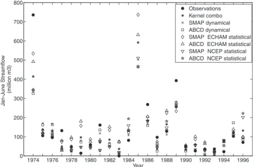
increased (more than 23 years). As the skill scores are already remarkably high for this region, it is exceptionally difficult to improve substantially over a single model hindcast. More distinct differences between single and multi-model approaches may be expected for regions of moderate to low skill. Fig-ure 11 portrays median seasonal streamflow from the six hydrological model ensembles and the kernel den-sity estimator multi-model combination, and the observations. Clearly the kernel combination does not produce the best estimate for any given year, but out-performs any single hydrological model approach over the hindcast period.
Streamflow forecast ensembles may also be used to construct probability density functions (PDFs), benefi-cial for risk-based decision making within the basin. As a demonstration, Figure 12 illustrates PDFs of sea-sonal streamflow from the pooling combination tech-nique and from the observed record (climatology) for 1991, a dry year. Actual 1991 streamflow is included as a dotted vertical line. The PDFs are estimated using a nonparametric kernel density estimator (Bowman and Azzalini, 1997). The pooled ensemble hindcast PDF is clearly shifted left of the climatological PDF, indicative of relatively less streamflow, more closely matching observed conditions. This type of information is useful for risk assessment and improved decision making con-cerning reservoir operations, water allocation, crop irrigation, etc.
SUMMARY AND DISCUSSION
Knowledge of forecast uncertainty stemming from climatic and hydrological models allows for improved forecasting and probabilistic evaluation within water resources decision making. Properly accounting for this uncertainty, however, remains a formidable chal-lenge. Little consideration has been given to stream-flow modeling methodologies that include coupling of both multiple climate and multiple hydrological mod-els, further increasing the pool of streamflow forecast ensemble members and accounting for cumulative sources of uncertainty. The framework presented here proposes integration and offline coupling of GCMs, multiple RCMs, and numerous hydrologic models to improve streamflow forecasting through generation of ensemble forecasts. For demonstration purposes, the framework is imposed on the Jaguaribe basin in northeastern Brazil for a hindcast of
1974-1996 monthly streamflow. The ECHAM4.5 and
NCEP⁄MRF9 GCMs are integrated with regional models, including dynamical and statistical models, and water balance models, specifically the SMAP and
TABLE 3. Skill Scores of Multi-Model Streamflow Hindcast Ensembles for 1974-1996.
Coupled Model
Correlation Coefficient
Root Mean Squared Error
RPSS Median Total
Pooled 0.90 90 - 0.21
Linear regression weighting
0.91 92 1,008 0.35
Kernel density estimator
0.92 90 962 0.55
Notes: RPSS, rank probability skill score. Pearson correlation coef-ficients use ensemble medians.
TABLE 2. Skill Scores of Hydrological Model Streamflow Hindcast Ensembles Over 1974-1996.
Coupled Model
Correlation Coefficient
Root Mean Squared
Error
RPSS Median Total
SMAP – Dynamical 0.88 100 1,707 0.42 ABCD – Dynamical 0.84 106 1,863 0.42 SMAP – Statistical ECHAM 0.90 81 962 )0.04 ABCD – Statistical ECHAM 0.88 88 1,069 )0.10
SMAP – Statistical NCEP 0.84 105 1,489 0.55 ABCD – Statistical NCEP 0.79 108 1,530 0.53
ABCD. Precipitation hindcasts from the GCMs are downscaled via the regional models and fed into the hydrological models, producing streamflow estima-tions. Multi-model ensemble combination techniques include pooling, linear regression weighting, and a kernel density estimator.
The kernel density estimator multi-model ensem-ble demonstrates superior skill considering numerous metrics in comparison with any single hydrological model approach (formulated from multi-climate
models). This improvement would only be expected to increase as the hindcast or forecast is lengthened (more than 23 years). It is anticipated that the coupled ABCD models, currently contributing little information, would also potentially receive greater weights under longer time-series. Their lack of weight for this case may be partially attributable to possible stability issues with kernel estimators at high dimensions, and requires further investigation. The respectable performance of the simple pooling combination approach is also noteworthy, but not unexpected, given the relatively short hindcast per-iod. The Jaguaribe basin clearly demonstrates high predictive skill, dampening potential improvements of multi-model approaches over single model forecasts. More distinct differences between single and multi-model approaches may be expected for regions of moderate to low skill.
The overall performance of the framework on the Jaguaribe basin appears robust in comparison with similar basin studies. It demonstrates an improvement over the Souza Filho and Porto (2003) ECHAM4.5-RSM-SMAP coupled model in terms of skill and uncertainty accounting. Souza Filho and Lall (2003) construct a semiparametric streamflow forecast model conditioned on an ENSO index and sea-surface tem-peratures, issuing forecasts for the January to May rainy season the prior July. The proposed framework produces similar skill, but differs by conducting a hind-cast with observed SSTs, issuing concurrent monthly forecasts. Although the framework proposed here is considerably more complex and multifaceted than the
FIGURE 11. Streamflow Hindcast Time-Series (1974-1996) With Median Seasonal Streamflow From the Six Hydrological Model Ensembles, From the Kernel Density Estimator Multi-Model Combination, and Observations.
FIGURE 12. Climatological (solid) and Pooled Ensemble Hindcast (dashed) PDFs for Total January to June, 1991, Streamflow.
semiparametric model, it does boast sufficient flexibil-ity for improvements at many stages, model substitu-tions, or other potential lines of analysis.
While the bulk of uncertainty is accounted for in the proposed framework, including initial conditions, model structure, and modeled processes, it is not entirely inclusive. To truly capture end-to-end uncer-tainty, two additional aspects must be targeted: model parameter and objective function uncertainty. The cur-rent framework can adequately capture model process uncertainty, but not explicitly model parameter uncer-tainty, specifically for hydrological models, although this may be simply addressed by calibrating the mod-els over various time periods and evaluating parame-ter ranges. Considering objective functions, model optimization in the current framework utilizes minimi-zation of model errors; alternative objective functions – independently or in combination – may better reflect existing uncertainty. These aspects are currently being developed for inclusion in the framework. Other on-going work utilizes the framework for apportioning uncertainty, comparing variances between single and multi-model approaches at each stage, to determine which processes or stages are contributing most signif-icantly to the overall uncertainty in the system.
Other aspects also warrant attention for future study, specifically multi-model combination tech-niques. Categorical forecasts (Rajagopalan et al., 2002) or providing prior information through Bayes-ian weights (Marshall et al., 2005; DelSole, 2006; Duan et al., 2006) provide attractive alternatives, and may assist in improving streamflow forecast skill.
APPENDIX I – VERIFICATION MEASURES
Total root mean square error:
TRMSEm¼
X
N
n¼1
ffiffiffiffiffiffiffiffiffiffiffiffiffiffiffiffiffiffiffiffiffiffiffiffiffiffiffiffiffiffiffiffiffiffiffiffiffiffi Pt
t¼1ðxo;t
xm;tÞ
2
t
s
ðA1Þ
Median root mean square error is identical, except-ing the summation and usexcept-ing ensemble medians.
Pearson’s correlation coefficient:
Rm¼
Pt
t¼1ðxm;t
xmÞðxo;t
xoÞ
ðt1Þr
mro
; ðA2Þ
where m is the model number, n is the ensemble members, xo,t is the observed streamflow value at
time t, xm,t is the hindcasted streamflow value, xo
and xm represent the observed mean and model ensemble median mean, respectively, and ro and rm are the observed and model ensemble median stan-dard deviations, respectively.
Rank Probability Skill Score
The rank probability skill score (RPSS) (Wilks, 1995; Sun et al., 2006; Block and Rajagopalan, 2008) is a measure of the skill of ensemble forecasts in com-parison with predictions by climatology forecasts. The general rank probability score (RPS) equation for any year takes the form
RPS¼X
R
m¼1
ðCPF;mCPO;mÞ
2
; ðA3Þ
where R is the number of categories (three in this study, i.e., above-, near-, and below-normal), and CPF,m and CPO,m are the cumulative predicted and observed probabilities, respectively, through category
m. For three categories of equal size, the climatolog-ical probability of being in each is 33%; for the cate-gory that is observed the probability is 100% and zero in the other two. Perfect forecasts result in RPS equal to zero. The RPSS is subsequently defined as
RPSS¼1 RPSFORECAST RPSCLIMATOLOGY
ðA4Þ
Rank probability skill score values range from )¥ to +1. A value of +1 represents perfect skill (i.e., a perfect forecast), while negative values symbolize poor skill; any value greater than zero corresponds to an improved forecast over climatology. The RPSS is calculated for each year.
ACKNOWLEDGMENT
LITERATURE CITED
Ajami, N.K., Q. Duan, X. Geo, and S. Sorooshian, 2006. Multi-Model Combination Techniques for Analysis of Hydrological Simulations: Application to Distributed Model Intercomparison Project Results. Journal of Hydrometeorology 8:755-768. Alley, W.M., 1984. On the Treatment of Evapotranspiration, Soil
Moisture Accounting, and Aquifer Recharge in Monthly Water Balance Models. Water Resources Research 20(8):1137-1149. Alley, W.M., 1985. Water Balance Models in One-Month-Ahead
Stream Flow Forecasting. Water Resources Research 21(4):597-606.
Barnston, A.G., Y. He, and M.H. Glantz, 1999a. Predictive Skill of Statistical and Dynamical Climate Models in Forecasts of SST During the 1997-1998 El Nino Episode and the 1998 La Nina Onset. Journal of Climate 12:217-244.
Barnston, A.G., A. Leetmaa, V.E. Kousky, R.E. Livezey, E. O’Lenic, H. Van den Dool, A.J. Wagner, and D.A. Unger, 1999b. NCEP Forecasts of the El Nino of 1997-1998 and its U.S. Impacts. Bulletin of the American Meteorological Society 80:1829-1852.
Barnston, A.G., S.J. Mason, L. Goddard, D.G. DeWitt, and S.E. Zebiak, 2003. Multi-Model Ensembling in Seasonal Climate Forecasting at IRI. Bulletin of the American Meteorological Society 84:1783-1796.
Beven, K., 2001. How Far Can We Go in Distributed Hydrological Modeling? Hydrology and Earth System Sciences 5(1):1-12. Beven, K. and J. Freer, 2001. Equifinality, Data Assimilation, and
Uncertainty Estimation in Mechanistic Modelling of Complex Environmental Systems Using the GLUE Methodology. Journal of Hydrology 249:11-29.
Bishop, C., 2006. Pattern Recognition and Machine Learning (Information Science and Statistics). Springer, Singapore. Block, P. and B. Rajagopalan, 2008. Statistical – Dynamical
Approach for Streamflow Modeling at Malakal, Sudan, On the White Nile River. Journal of Hydrologic Engineering 14(2):185-196.
Bowman, A. and A. Azzalini, 1997. Applied Smoothing Techniques for Data Analysis. Oxford University Press, New York.
Cane, M.A., S.E. Zebiak SE, and S.C. Dolan, 1986. Experimental Forecasts of El-Nino. Nature 321:827-832.
Chowdhury, S. and A. Sharma, 2008. Long Range NINO3.4 Predic-tions Using Pair Wise Dynamic CombinaPredic-tions of Multiple Mod-els. Journal of Climate 22(3):793-805.
COGERH (Companhia de Gesta˜o dos Recursos Hı´dricos), 1998. Plano de Gerenciamento da Bacia do Rio Jaguaribe [In Portu-guese]. Companhia de Gesta˜o dos Recursos Hı´dricos, Fortaleza, Ceara´, Brazil.
DelSole, T., 2006. A Bayesian Framework for Multimodel Regres-sion. Center for Ocean-Land-Atmosphere Studies. ftp://grads. iges.org/pub/delsole/dir_multimodel/multimodellr.pdf, accessed December 2007.
Devineni, N., A. Sankarasubramanian, and S. Ghosh, 2008. Multi-model Ensembles of Streamflow Forecasts: Role of Predictor State in Developing Optimal Combinations. Water Resources Research 44, W09404, doi: 10.1029/2006WR005855.
Doblas-Reyes, F.J., M. Deque, and J.P. Piedelievre, 2000. Multi-Model Spread and Probabilistic Seasonal Forecasts in PRO-VOST. Quarterly Journal of the Royal Meteorological Society 126:2069-2088.
Doblas-Reyes, F.J., R. Hagedorn, and T.N. Palmer, 2005. The Rea-tionale Behind the Success of Multi-Model Ensembles in Sea-sonal Forecasting – II. Calibration and Combination. Tellus 57A:234-252.
Duan, Q., N.K. Ajami, X. Gao, and S. Sorooshian, 2006. Multi-Model Ensemble Hydrologic Prediction Using Bayesian Multi-Model Averaging. Advances in Water Resources 30:1371-1386.
Fritsch, J.M., J. Hilliker, J. Ross, and R.L. Vislocky, 2000. Model Consensus. Weather Forecasting 15:571-582.
Georgakakos, K.P., D.J. Seo, H. Gupta, J. Schake, and M.B. Butts, 2004. Characterizing Streamflow Simulation Uncertainty Through Multimodel Ensembles. Journal of Hydrology 298(1-4):222-241.
Goddard, L., S.J. Mason, S.E. Zebiak, C.F. Ropelewski, R. Basher, and M.A. Cane, 2001. Current Approaches to Seasonal-to-Inter-annual Climate Predictions. International Journal of Climatol-ogy 21:1111-1152.
Hagedorn, R., 2001. Development of a Multi-Model Ensemble Sys-tem for Seasonal to Interannual Prediction. Proceedings XXVI General Assembly of the EGS, Nice, European Geophysical Soci-ety, France.
Hagedorn, R., F.J. Doblas-Reyes, and T.N. Palmer, 2005. The Rationale Behind the Success of Multi-Model Ensembles in Seasonal Forecasting. Part I: Basic Concept. Tellus 57A:219-233.
Hamill, T., 2001. Interpretation of Rank Histograms for Verifying Ensemble Forecasts. Monthly Weather Review 129:550-560. Harrison, M.S.J., T.N. Palmer, D.S. Richardson, R. Buizza, and T.
Petroliagis, 1995. Joint Ensembles From the UKMO and ECMWF Models.In:ECMWF Seminar Proceedings: Predictabil-ity, Vol. 2, ECMWF, Reading, United Kingdom, pp. 61-120. Hastenrath, S. and L. Heller, 1977. Dynamics of Climate Hazards
in Northeast Brazil. Quarterly Journal of the Royal Meteorologi-cal Society 103:77-92.
Ines, A.V.M. and J. Hansen, 2006. Bias Correction of Daily GCM Rainfall for Crop Simulation Studies. Agricultureal and Forest Meteorology 138(1-4):44-53.
Juang, H.-M.H., S.-Y. Hong, and M. Kanamitsu, 1997. The NCEP Regional Spectral Model: An Update. Bulletin of the America Meteorological Society 78:2125-2143.
Juang, H.-M.H. and M. Kanamitsu, 1994. The NMC Nested Regio-nal Spectral Model. Monthly Weather Review 122:3-26.
Kang, I.S. and J.H. Yoo, 2006. Examination of Multi-Model Ensem-ble Seasonal Prediction Methods Using a Simple Climate Sys-tem. Climate Dynamics 26:285-294.
Krishnamurti, T.N., C.M. Kishtawal, T.E. LaRow, D.R. Bachiochi, Z. Zhang, C.E. Williford, S. Gadgil, and S. Surendran, 1999. Improved Weather and Seasonal Climate Forecasts From Multi-Model Superensemble. Science 285:1548-1550.
Krishnamurti, T.N., C.M. Kishtawal, Z. Zhang, T.E. LaRow, D.R. Bachiochi, C.E. Williford, S. Gadgil, and S. Surendran, 2000. Multimodel Ensemble Forecasts for Weather and Seasonal Cli-mate. Journal of Climate 13:4196-4216.
Kumar, A., A.G. Barnston, and M.P. Hoerling, 2001. Seasonal Pre-dictions, Probabilistic Verifications, and Ensemble Size. Journal of Climate 14:1671-1676.
Kumar, A., M.P. Hoerling, M. Ji, A. Leetmaa, and P. Sard-eshmukh, 1996. Assessing a GCM’s Suitability for Making Sea-sonal Predictions. Journal of Climate 9:115-129.
Landman, W.A., S.J. Mason, P.D. Tyson, and W.J. Tennant, 2001. Statistical Downscaling of GCM Simulations to Streamflow. Journal of Hydrology 252:221-236.
Livezey, R. E., M. Masutani, and M. Ji, 1996. SST-Forced Seasonal Simulation and Prediction Skill for Versions of the NCEP⁄MRF Model. Bulletin of the American Meteorological Society 77:507-517.
Lopes, J.E.G., B.P.F. Braga, and J.G.L. Conejo, 1982. SMAP – A Simplified Hydrological Model. In:Applied Modeling in Catch-ment Hydrology, V.P. Singh (Editor). Water Resources Publica-tions, Littleton, Colorado, pp. 167-176.
Marshall, L., D. Nott, and A. Sharma, 2005. Hydrological Model Selection: A Bayesian Alternative. Water Resources Research 41, doi: 10.1029/2004WR003719.
Mason, S.J., L. Goddard, N.E. Graham, E. Yulaeva, L. Sun, and P.A. Arkin, 1999. The IRI Seasonal Climate Prediction System and the 1997⁄1998 El Nino Event. Bulletin of the American Meteorological Society 80:1853-1973.
McLeod, A.I., D.J. Noakes, K.W. Hipel, and R.M. Thompstone, 1987. Combining Hydrologic Forecasts. Journal of Water Resources Planning and Management 113(1):29-41.
Moura, A.D. and J. Shukla, 1981. On the Dynamics of Droughts in Northeast Brazil: Observations, Theory, and Numerical Experi-ments With a General Circulation Model. Journal of Atmo-spheric Sciences 38:2653-2675.
Mujumdar, P.P. and S. Ghosh, 2008. Modeling GCM and Scenario Uncertainty Using a Possibilistic Approach: Application to the Mahanadi River, India. Water Resources Research 44:W06407, doi: 10.1029/2007WR006137.
Murphy, J., 1999. An Evaluation of Statistical and Dynamical Techniques for Downscaling Local Climate. Journal of Climate 12(8):2256-2284.
Palmer, T.N., A. Alessandri, U. Andersen, P. Cantelaube, M. Davey, P. De´le´cluse, M. De´que´, E. Die´z, F.J. Doblas-Reyes, H. Feddersen, R. Graham, S. Gualdi, J.-F. Gue´re´my, R. Hagedorn, M. Hoshen, N. Keenlyside, M. Latif, A. Lazar, E. Maisonnave, V. Marletto, A.P. Morse, B. Orfila, P. Rogel, J.-M. Terres, and M.C. Thomson, 2004. Development of a European Multi-Model Ensemble System for Seasonal to Interannual Prediction (DEMETER). Bulletin of the American Meteorological Society 85:853-872.
Palmer, T.N., C. Brankovic, and D.S. Richardson, 2000. A Probabil-ity and Decision-Model Analysis of PROVOST Seasonal Multi-Model Ensemble Integrations. Quarterly Journal of the Royal Meteorological Society 126:2013-2034.
Raftery, A.E., D. Madigan, and J.A. Hoeting, 1997. Bayesian Model Averaging for Linear Regression Models. Journal of the Ameri-can Statistical Association 92(437):179-191.
Rajagopalan, B., U. Lall, and S.E. Zebiak, 2002. Categorical Cli-mate Forecasts Through Regularization and Optimal Combina-tion of Multiple GCM Ensembles. Monthly Weather Review 130:1792-1811.
Reed, S., V. Koren, M. Smith, Z. Zhang, F. Moreda, J.D. Seo, and DMIP Participants, 2004. Overall Distributed Modeling Inter-comparison Project Results. Journal of Hydrology 298(1-4):27-60.
Regonda, S., B. Rajagopalan, M. Clark, and E. Zagona, 2006. A Mul-timodel Ensemble Forecast Framework: Application to Spring Seasonal Flows in the Gunnison River Basin. Water Resources Research 42, doi: 10.1029/2005WR004653.
Robertson, A.W., U. Lall, S.E. Zebiak, and L. Goddard, 2004. Improved Combination of Multiple Atmospheric GCM Ensem-bles for Seasonal Prediction. Monthly Weather Review 132:2732-2744.
Roeckner, E., K. Arpe, L. Bengtsson, M. Christoph, M. Claussen, L. Duemenil, M. Esch, M. Giorgetta, U. Schlese, and U. Schulz-weida, 1996. The Atmospheric General Circulation Model Echam4: Model Description and Simulation of Present-Day Cli-mate. Max-Planck-Institut fur Meteorologie Max-Planck-Institut fur Meteorologie Rep. 218, Hamburg, Germany.
Russo, R., A. Peano, I. Becchi, and G.A. Bemporad, 1994. Advances in Distributed Hydrology. Water Resources Publications, Chel-sea, Michigan.
Saha, S., S. Nadiga, C. Thiaw, and J. Wang, 2006. The NCEP Cli-mate Forecast System. Journal of CliCli-mate 19(15):3483-3517. Shamseldin, A.Y. and K.M. O’Connor, 1999. A Real-Time
Combina-tion Method for the Outputs of Different Rainfall-Runoff Mod-els. Hydrological Science Journal 44(6):895-912.
Smith, M.B., D.J. Seo, V.I. Koren, S. Reed, Z. Zhang, Q. Duan, R. Moreda, and S. Cong, 2004. The Distributed Model Intercom-parison Project (DMIP): An Overview. Journal of Hydrology 298(1-4):4-26.
Souza Filho, F.A. and U. Lall, 2003. Seasonal to Interannual Ensemble Streamflow Forecasts for Ceara, Brazil: Applications of a Multivariate, Semiparametric Algorithm. Water Resources Research 39(11):1307, doi: 10.1029/2002WR001373.
Souza Filho, F.A. and R.L.L. Porto, 2003. Acoplamento de Modelo Clima´tico e Modelo Hidrolo´gico. In: XV Simpo´sio Brasileiro de Recursos Hı´dricos, 2003, Curitiba⁄PR. Anais do XV Simpo´sio Brasileiro de Recursos Hı´dricos. ABRH, Porto Alegre⁄RS (Proce-dure in Portuguese).
Stern, W. and K. Miyakoda, 1995. Feasibility of Seasonal Forecasts Inferred From Multiple GCM Simulations. Journal of Climate 8(5):1071-1085.
Sun, L., D.F. Moncunill, H. Li, A.D. Moura, and F.A. Souza Filho, 2005. Climate Downscaling Over Nordeste Brazil Using NCEP RSM97. Journal of Climate 18:551-567.
Sun, L., D.F. Moncunill, H. Li, A.D. Moura, F.A. Souza Filho, and S.E. Zebiak, 2006. An Operational Dynamical Downscaling Pre-diction System for Nordeste Brazil and the 2002-04 Real-Time Forecast Evaluation. Journal of Climate 19:1990-2007.
Tebaldi, C., R. Smith, D. Nychka, and L.O. Mearns, 2005. Quanti-fying Uncertainty in Projections of Regional Climate Change: A Bayesian Approach to the Analysis of Multi-Model Ensembles. Journal of Climate 18:1524-1540.
Thomas, H.A., 1981. Improved Methods for National Water Assess-ment. Report, contract WR 15249270. U.S. Water Resources Council, Washington, D.C.
Thomas, H.A., C.M. Marin, M.J. Brown, and M. B Fiering, 1983. Methodology for Water Resource Assessment Report to U.S. Geological Survey. Rep. NTIS 84-124163, National Technical Information Service, Springfield, Virginia.
Tracton, M.S. and E. Kalnay, 1993. Operational Ensemble Predic-tion at the NaPredic-tional Meteorological Center: Practical Aspects. Weather Forecasting 8:379-398.
Vandewiele, G.L., C.-Y. Xu, and Ni-Lar-Win, 1992. Methodology and Comparative Study of Monthly Water Balance Models in Belgium, China and Burma. Journal of Hydrology 134:315-347. Vieux, B.A., 2001. Distributed Hydrologic Modeling Using GIS.
Kluwer Academic Publishers, Dordrecht, the Netherlands. Von Storch, H. and F.W. Zwiers, 1999. Statistical Analysis in
Cli-mate Research. Cambridge University Press, Cambridge, United Kingdom.
Ward, M.N. and C.K. Folland, 1991. Prediction of Seasonal Rainfall in the North Nordeste of Brazil Using Eigenvectors of sea Sur-face Temperature. International Journal of Climatology 11:711-743.
Wilby, R.L., T.M.L. Wigley, D. Conway, P.D. Jones, B.C. Hewitson, J. Main, and D.S. Wilks, 1998. Statistical Downscaling of General Circulation Model Output: A Comparison of Methods. Water Resources Research 34(11):2995-3008, doi: 10.1029/98 WR02577.
Wilks, D., 1995. Statistical Methods in Atmospheric Science: An Introduction. Academic Press, San Diego, California.
Yun, W.T., L. Stefanova, A.K. Mitra, T.S.V. Vijay Kumar, W. Dewar, and T.N. Krishnamurti, 2005. A Multi-Model Superen-semble Algorithm for Seasonal Climate Prediction Using DEMETER Forecasts. Tellus 57A:280-289.