www.nat-hazards-earth-syst-sci.net/14/2655/2014/ doi:10.5194/nhess-14-2655-2014
© Author(s) 2014. CC Attribution 3.0 License.
Methodology for flood frequency estimations in small catchments
V. David and T. Davidova
Department of Irrigation, Drainage and Landscape Engineering, Faculty of Civil Engineering, Czech Technical University in Prague, Prague, Czech Republic
Correspondence to:V. David ([email protected])
Received: 24 September 2013 – Published in Nat. Hazards Earth Syst. Sci. Discuss.: 8 November 2013 Revised: 31 August 2014 – Accepted: 2 September 2014 – Published: 1 October 2014
Abstract. Estimations of flood frequencies in small catch-ments are difficult due to a lack of measured discharge data. This problem is usually solved in the Czech Republic by hy-drologic modelling when there is a reason not to use the data provided by the Czech hydrometeorological institute, which are quite expensive and have a very low level of accuracy. Another way is to use a simple method which provides suf-ficient estimates of flood frequency based on the available spatial data. A new methodology is being developed consid-ering all important factors affecting flood formation in small catchments. The relationship between catchment descriptors and flood characteristics has been analysed first to get an overview of the importance of each considered descriptor. The results for different descriptors vary from a highly cor-related relationship of an expected shape to a relationship which is opposite to that expected, mainly in the case of land use. The parameterisation of the methodology is also pre-sented, including the sensitivity tests on each involved catch-ment descriptor and cross-validation of achieved results. In its present form, the methodology achieves anRadj2 value of about 0.61 for 10- and 0.60 for 100-year return periods.
1 Introduction
A methodology for the estimations of flood frequency in small catchments is being developed. The reason for the pre-sented research is mainly the fact that engineers often need quick instant design flood estimates for the purposes of dif-ferent feasibility studies. It usually takes at least one month to obtain such estimates from the official provider, and the data can be relatively expensive. It is also important to take into consideration the fact that provided design floods have a relatively low level of accuracy. The uncertainty of the data
for small catchments which are usually ungauged is up to ±60 % in the 4th class of accuracy according to Czech stan-dards (Kulasová and Holík, 1997). This means that use of the data should take into consideration its uncertainty and that it is appropriate to apply correction coefficients in cases of higher safety demands.
The approach used for the development of the presented methodology in general applies similarity principles which have been discussed by many authors worldwide (Burn, 1997; Merz and Blöschl, 2005; Wagener et al., 2007; Patil and Stieglitz, 2012). These principles are usually applied in three ways: (i) for the direct estimation of flood quantiles, (ii) for the estimation of probability distribution parameters and (iii) for the estimation of hydrologic model parameters. The methodology proposed in this study adopts the first op-tion in order to be applicable by practical engineers who may be unfamiliar with the application of more advanced statisti-cal analysis methods or hydrologic models.
There are different regression-based methods which are similar to the method proposed by the authors of this pa-per. These methods adopt different procedures for param-eter estimation, such as ordinary least square regression (OLS), weighted least square regression (WLS), and gen-eralised least square regression (GLS), which is discussed by Stedinger and Tasker (1985) and further by Pandey and Nguyen (1999), who involved more parameter estima-tion methods such as least absolute value regression, ro-bust regression and others. These methods are further im-proved by the involvement of a Bayesian framework ap-proach and Monte Carlo simulations (Haddad and Rahman, 2012; Haddad et al., 2012; Micevski and Kuczera, 2009).
choose more suitable parts of the power function (according to its slope and curvature), but on the other hand, it avoids the linearisation of the problem by logarithmic transforma-tion. The mentioned general shape can also lead to too high a number of model parameters, which could make the model insufficiently robust, which corresponds to results presented by Perrin et al. (2001) for continuous models. Thus, the shifts were excluded in the first step of model development pre-sented in this paper, and will be included in the next step.
2 Overview of the proposed methodology
The proposed methodology is based on the calculation of flood frequencies using catchment descriptors. The proce-dure is derived using GIS tools and spatial data analysis. The method should be applicable to any small catchment in the Czech Republic for which the input data are available. The initial list of catchment descriptors which are considered im-portant for flood formation is as follows:
– catchment area,
– storm rainfall characteristics, – slope conditions of the catchment, – catchment shape,
– land use, – soil properties.
This list corresponds in general to the list used by Sefton and Howarth (1998) for their study, and involves both physi-cal geographic and climate properties as discussed by Berger and Entekhabi (2001). Berger and Entekhabi (2001) did an analysis of the long-term basin response, but it can be ex-pected that it is even more necessary to involve both types of information in flood response assessment. The list also contains types of parameters used for the purpose of max-imum possible flood calculation by Reed and Field (1992). Eng et al. (2007) did the analysis of the combination of catchment characteristics with the geographic region-of-influence approach, resulting in better model performance. Nezhad et al. (2010) also used geographic information to-gether with climatic characteristics for flood frequency anal-ysis, and applied the residual kriging in physiographical space for quantile estimation using canonical correlation analysis. However, geographic location was not included in the presented analysis, because it is considered to have an in-direct influence on flood discharge values, and the emphasis was put on catchment descriptors for which a direct influence is expected.
First, the procedure for the calculation of catchment de-scriptors was defined, including the necessary input data lay-ers. The most important input is the digital elevation model (DEM), which is sufficient input for the calculation of the
catchment area, the average slope and the catchment shape. This is a relatively easily available data source, and the proce-dures for its processing for purposes of hydrologic analyses have been broadly published. The situation is quite different in the case of the calculation of other descriptors. There are different reasons for the difficulties in the data acquisition and processing. There are many different sources of land use data which differ in many aspects, mainly the resolution, ac-curacy and information content. Moreover, there are no lay-ers available containing storm rainfall characteristics or gap-less soil maps containing sufficient information for the infil-tration properties assessment. This is why the analysis of the influence of soil properties could not yet be done and why there was a need to prepare rainfall characteristic maps.
The general construction of the proposed methodology consisting in the multiplication of power functions of catch-ment descriptors and the choice of catchcatch-ment descriptors is similar to those published for example by Asquith and Slade (1996) or Olson (2009) for conditions of regions in the United States, or by Jaafar et al. (2011) for conditions in the southwest of England. In general, the value is calculated as a product of functions of single catchment descriptors as described by the equation
QN=a0·Y
i
fi(CDi)+d0, (1)
whereQN is flood discharge with the return period of N
years,a0andd0are correction parameters,fiare
mathemat-ical functions and CDi are catchment descriptors.
The function for the calculation of each component of Eq. (1) is in general considered a power function, with shifts in both directions in the form of
fi(CDi)=ai·(bi+CDi)ci+di, (2)
whereai,bi,ci anddi are parameters of mathematical
func-tions fi. Shifts are driven by parameters bi anddi.
Equa-tion (1) then becomes QN=a0·Y
i
ai·(bi+CDi)ci+di+d0, (3)
which can be rewritten as QN=a′0·
Y
i
(bi+CDi)ci+di′
+d0, (4)
where a0′ =a0·Y
i
ai anddi′= di ai
. (5)
When the simple power function is considered, which is usual for similar applications and considered more robust, the values ofbi anddi are equal to 0. The simplified form of
Eq. (4) then becomes QN=a′0·
Y
i
3 Assessment of the relationship between catchment descriptors and flood discharges
Discharges with different return periods published by Zítek (1970) were used for the analysis. The data pub-lished in this book were derived based on a time series from 250 gauging stations spread over the whole area of the former Czechoslovakia. The shortest length considered for the anal-ysis was 25 years, while the median is 43 years. These data are based only on years containing no gaps, which means that years containing gaps in records were excluded from quantile calculations.
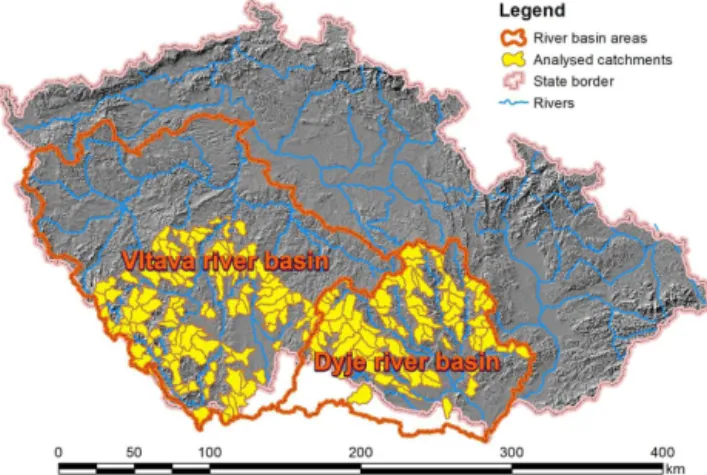
A subset of 196 catchments with a catchment area (A) less than 150 km2located in the Vltava River basin and the Dyje River basin (see Fig. 1), for which the flood frequency data are published by Zítek (1970), was chosen for the analysis. Catchments were delineated using a layer containing fourth-order catchments available from the Water Research Institute and elevation data to get polygons for calculations of catch-ment descriptor values.
The calculation procedure was different for each consid-ered catchment descriptor. The simplest one is the calculation of the descriptor related to the catchment slope (s), which is calculated as the average slope from the layer containing slopes calculated based on the analysis of DEM. DEM is also input for the calculation of the catchment descriptor related to catchment shape. For this purpose, shape factor – SF – was used, which is defined as the drainage area divided by the square of the longest flow path. This descriptor was cho-sen based on previous research (David, 2011). The longest flow path for each catchment was calculated using standard GIS procedures (flow direction and flow length), while the catchment area was calculated simply from the geometry of each catchment polygon.
For the calculation of the descriptor related to storm rain-fall layers containing information on the value of maximum 24 h precipitation (P), totals for the considered return peri-ods needed to be prepared. They were interpolated from point data digitised based on the information for each gauging sta-tion published by Šamaj et al. (1985). The descriptor for each catchment was then calculated as an average value over the catchment area.
Land use was analysed using a curve number parameter (CN) published by, among others, Mishra and Singh (2003). This parameter originally combines the information on land use and soil infiltration properties. However, the spatial dis-tribution was considered only with respect to land use, while soil information was considered spatially homogeneous and corresponding to hydrological soil group B, in order to be able to assess land use influence on flood discharges separately.
The analyses focusing on the relationship between catch-ment descriptors and flood discharges were performed in-dividually for each of the considered catchment descrip-tors. For this paper, flood discharge with return periods of
Figure 1.Catchments less than 150 km2selected for the analysis.
T=10 years andT=100 years were selected as in the case of the study published by Pandey and Nguyen (1999). Cor-relations between dependent and exploratory variables were analysed using parameter optimisation for Eq. (2).
3.1 Analyses of the correlation between catchment descriptors and flood discharges
Basic analyses were performed by relating the value of the catchment descriptor directly to the value of the flood dis-charge within the given return period. The assumption is that there should be a significant relationship between the catch-ment area and the peak discharge value and between the pre-cipitation total for a given return period and the peak dis-charge value related to the same return period.
3.1.1 Catchment area
The catchment area is considered the most important catch-ment descriptor. It is assumed that the value of flood dis-charge increases with an increasing catchment area. How-ever, it is usually also assumed that the relationship between the catchment area and flood discharge is not linear in small catchments (Sivapalan et al., 2002). The main reason con-sists in the spatial distribution of storm rainfalls, which are the most frequent causes of floods in small catchments in the conditions of the Czech Republic.
Areas of catchments involved in the analyses vary in range from 7.7 to 146.4 km2with a mean value of 58.2 km2. More
than 51 % of catchments are smaller than 50 km2, and more
than 87 % are smaller than 100 km2.
Figure 2.Relationship between catchment area and peak discharge value forT=10 years (left panel) andT=100 years (right panel) with fitted lines following Eq. (2).
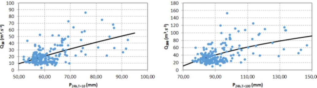
Figure 3.Relationship between catchment average maximum 24 h precipitation total and peak discharge values forT=10 years (left panel) andT=100 years (right panel) with fitted lines following Eq. (2).
3.1.2 Maximum 24 h precipitation total
The precipitation total, together with the catchment area, is considered the most important factor affecting flood dis-charge values. The product of the precipitation total and catchment area can be understood as the volume of water available for runoff. Thus, the value of peak discharge is con-sidered increasing with an increasing precipitation total, but the relationship is not considered linear, as lower values of precipitation totals are in general more affected by losses. Values of maximum 24 h precipitation totals for different re-turn periods are the only data source which is available as a continuous map for the whole area of the Czech Republic, and therefore this characteristic was used for the analysis, al-though floods are usually caused by precipitation events with a duration shorter than 24 h.
Interpolated values of maximum 24 h precipitation within the sample vary in range from 51.9 to 92.3 mm in the case of a 10-year return period and from 75.8 to 146.8 mm in the case of a 100-year return period. Average values are 61.9 and 92.6 mm, respectively. However, most catchments have val-ues of a maximum 24 h precipitation total in a very narrow range, which is from 55 to 65 mm for more than 72 % in the case of a 10-year return period, and from 80 to 95 mm in the case of a 100-year return period.
The results show that the relationship between the max-imum 24 h precipitation total and peak discharge value for T =10 years follows almost a straight line (see Fig. 3). Achieved values of R2 are higher than for the catchment
area, i.e. R2=0.32 for T =10 years and R2= 0.27 for T=100 years.
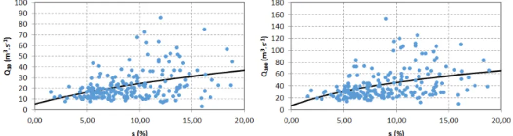
3.1.3 Average slope of the catchment
Catchment slope conditions are considered important mainly due to their influence on overland flow velocities. A higher slope of the catchment leads to faster concentrations and con-sequently to higher values of peak discharge.
Slope conditions in catchments involved in the analysis vary in a relatively wide range from flat to mountainous ar-eas. The average slope (s) ranges from 1.5 to 18.8 %, but 60 % have a value in the range from 4 to 10 %.
Results of performed analyses confirm the assumption of increasing peak discharge values with increasing average slope of the catchment. Results presented in Fig. 4 show the almost straight shape of a fitted curve. Values of the deter-mination coefficient achieved by parameter optimisation are R2=0.15 forT=10 years andR2=0.14 forT=100 years. 3.1.4 Catchment shape
Catchment shape affects flood discharges through the runoff concentration. It is assumed that wide catchments (fan shaped) have higher values of peak discharges than narrow oblong catchments (fern shaped), which is published, among others, by Murthy (2002). According to the definition of SF, the values are higher for fan-shaped catchments than for fern-shaped catchments.
Figure 4.Relationship between catchment average slope and peak discharge value forT=10 years (left panel) andT=100 years (right panel) with fitted lines following Eq. (2).
Figure 5.Relationship between catchment shape factor and peak discharge value forT=10 years (left panel) andT=100 years (right panel) with fitted lines following Eq. (2).
the case for the sample used for the analysis, where the max-imum value is SF=0.57, while the minimum is 0.10. How-ever, most catchments (75 %) have a value of SF below 0.22. Results obtained by the basic analyses performed are in opposition to those expected. These results are shown in Fig. 5. Fitted curves have a shape representing a decreasing value of flood discharge with an increasing value of SF. How-ever, coefficients of determination are very low: R2=0.02 for T =10 years as well as forT =100 years, which indi-cates no match between this catchment descriptor and peak discharge.
The results shown do not necessarily refute the mentioned principles. This can be caused by a stronger influence of other factors. Therefore, further analyses had to be performed of the influence of this catchment property.
3.1.5 Land use
Land use affects flood discharges in different ways. Mainly, precipitation losses caused by interception and infiltration and affection of routing speed by the surface roughness are important. For the purposes of the presented analyses, the CN value was chosen as a catchment descriptor. This param-eter was designed to calculate direct runoff, which means that it affects flood discharge values through the volume of runoff. It reaches values from 0 to 100. A zero value cor-responds to no runoff, while a value of 100 corcor-responds to the maximum runoff. This means that peak discharge should increase with an increasing CN value. CN values were cal-culated from maps derived for the whole area considered
covered by hydrological soil group B to exclude the influ-ence of soil conditions.
In the sample of catchments used in this study, the values of CN range from 62.1 to 80.9.
Results of performed basic analyses are again opposite to the meaning of the CN parameter. The trend is decreasing in both cases shown in Fig. 6. The determination is furthermore relatively high, i.e.R2=0.28 forT =10 andR2=0.26 for T=100 years.
There are several possible reasons for such results. First, the influence of land use can be weaker than the influence of other factors, which cannot be avoided in this type of analy-sis. Second, areas of land use types with low values of CN, such as forests, are usually concentrated in hilly and moun-tainous areas, which typically have high and intense storm rainfall and consequently high values of flood discharges.
3.2 Additional analyses of the correlation between catchment descriptors and flood discharges
Figure 6.Relationship between catchment average CN value and peak discharge value forT=10 years (left panel) andT=100 years (right panel) with fitted lines following Eq. (2).
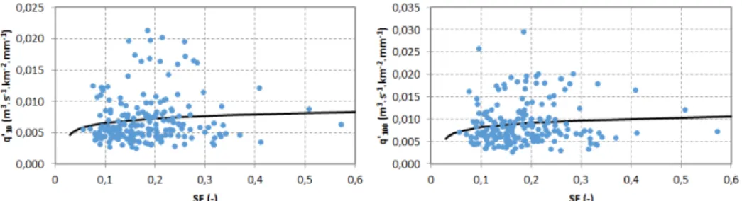
Figure 7. Relationship between catchment average shape factor and peak discharge value per unit area and unit precipitation total for
T =10 years (left panel) andT=100 years (right panel) with fitted lines following Eq. (2).
Figure 8. Relationship between catchment average CN value and peak discharge value per unit area and unit precipitation total for
T =10 years (left panel) andT=100 years (right panel) with fitted lines following Eq. (2).
catchment descriptors and the flood discharge divided by the product of the catchment area and the precipitation total. 3.2.1 Catchment shape
Results of the comparison of shape factor and flood discharge divided by the product of the catchment area and the precip-itation total show a growing trend (see Fig. 7). This corre-sponds to the assumption that flood discharge values increase with increasing values of the shape factor.
The trend obtained by fitting the curve shaped accord-ing to the equation is not very significant, havaccord-ing a value ofR2=0.01 forT=10 years as well as forT =100 years, which again indicates no match. This results in the suppo-sition that this catchment descriptor probably cannot signif-icantly increase the performance of the proposed methodol-ogy for estimations of flood discharges.
3.2.2 Land use
In the case of land use represented by the CN value, the re-sults of the comparison with flood discharge divided by the catchment area and precipitation total are similar to those ob-tained by the basic analysis. It shows an inverted proportion of peak discharge values per unit and unit precipitation to the value of CN in both cases, which is again opposite to the definition of the CN parameter.
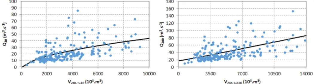
Figure 9.Relationship between catchment 24 h precipitation volume and peak discharge value forT=10 years (left panel) andT=100 years (right panel) with fitted lines following Eq. (2).
3.2.3 Available volume
To make a simple check of the influence of the two param-eters providing the best performance, the assessment of the relationship between available volumes of the maximum 24 h precipitation total and peak discharge values was performed. The volume was calculated as a product of the precipitation total and the catchment area, which were identified as the most important catchment descriptors.
The results of this analysis show that the performance of the calculation based on this parameter does not provide im-portant improvement with respect to the value of the maxi-mum 24 h precipitation total for the given return period. The value of the determination coefficient is a bit higher in the case of the 100-year return period (R2=0.33). In the case of the 10-year return period, the value of the determination co-efficient is lower (R2=0.30) than for the application of the 24 h precipitation total alone.
4 Methodology parameterisation and validation The calibration was carried out for the simpler form of a power function to get the results for a more robust calcu-lation procedure. In this case, the OLS method was used for a log-transformed equation. The shape of the equation after this transformation is as follows:
logQN=loga0′+
X
i
ci·log CDi. (7)
Parameter values were then estimated using the equation
β=CDT ·CD−1·CDT ·X, (8) whereβis a vector of equation parameter estimators (loga′
0, c1, . . . ,cm),CDis a matrix of catchment descriptor
loga-rithms with the first column filled by 1, andXis a vector of
flood discharge value logarithms.
The methodology was first parameterised using the whole data set for all tested catchment descriptors including also the land use descriptor and shape factor, which did not provide good results when analysed individually. The parameterisa-tion was then carried out again without considering the least
important descriptors (those having the weakest individual correlation to design flood values) to assess if they can be excluded from the calculation without loss of model perfor-mance. Parameters were always recalibrated after removing any descriptor. Land use and shape factor were identified as the least significant descriptors according to the results pre-sented in previous analyses. Thus, each of them was individ-ually removed from the complete set of descriptors, and pa-rameters for all other descriptors were recalibrated. Further-more, both mentioned descriptors were removed, and finally also catchment slope descriptor was removed. Values of the tstatistic were then calculated for each of mentioned combi-nations in order to assess the significance of each catchment descriptor in a quantitative way.
The results of parameterisation were assessed using a de-termination coefficient (R2) and an adjusted value of deter-mination coefficient (Radj2 ) calculated as
R2=1− n
P
i=1
Qobs,i−Qest,i2
n
P
i=1
Qobs,i−Qobs2
(9)
Radj2 =1− n−1 n−1−K·
1−R2, (10)
whereQobs,iis theT =10-year orT=100-year design flood value,Qest,iis the estimated design flood value, andQobsis an average of all design flood values in the data set.
Table 1.Values of RMSE and MAE for all considered combinations of involved catchment descriptors.
Return periodN 10 years 100 years
Considered RMSE MAE RMSE MAE
catchment (m3s−1) (m3s−1) (m3s−1) (m3s−1)
descriptors
A,P 9.57 6.10 17.88 12.16
A,P,s 9.28 5.80 17.17 11.35 A,P,s, CN 8.71 5.48 15.76 10.53 A,P,s, SF 9.21 5.78 17.17 11.33 A,P,s, SF, CN 8.64 5.41 15.78 10.42
considered catchment descriptors improves the performance of the proposed methodology, but the involvement of SF im-proves the performance only very little. Moreover, the values of the t statistic (tc4) related to SF are not high enough to reject the null hypothesis (c4=0) in both cases where SF is involved in the regression forT=100 years and in one case for T=10 years at a level of 0.05 (see Table 4). Thus, this parameter will not be considered for further development.
There is a variety of methods which can be used for vali-dation in case of a lack of valivali-dation data. These are mainly Monte Carlo (Haddad et al., 2013), leave-one-out (Jaafar et al., 2011) ork-fold cross-validation. In this case, thek-fold cross-validation method was used, which is based on splitting the data set into k similarly large subsamples and running the calibration and validationktimes when using always one subsample for validation while using the others together for calibration. For the purpose of this study, the value ofk=7 was chosen. The data set was divided into folds randomly to avoid distortion of results. Values of the determination coef-ficient as well as other performance metrics were calculated for both the training and validation data set in the case of each fold. These were then compared to values obtained by the calibration using the whole data set.
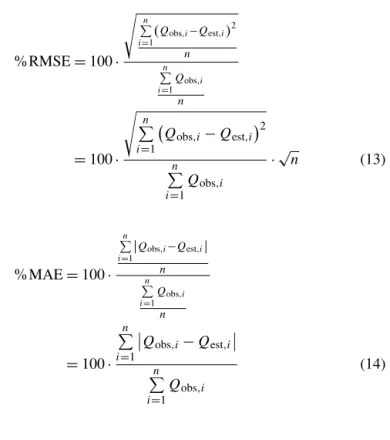
As measures of performance, root mean square error (RMSE) and mean absolute error (MAE) values which are both discussed by Willmott and Matsuura (2005) were used for each considered combination of catchment descriptors – see Eqs. (10) and (11). Additionally, relative values of RMSE and MAE were used – % RMSE and % MAE – expressed as shown by Eqs. (12) and (13). Finally, bias was calculated for the calibration using the whole data set as well as for folds to make a check on the bias of estimated values resulting from logarithmic transformation (McCuen et al., 1990).
RMSE= v u u u t n P
i=1
Qobs,i−Qest,i2
n (11)
MAE=
n
P
i=1
Qobs,i−Qest,i
n (12)
Table 2.Values of % RMSE and % MAE for all considered combi-nations of involved catchment descriptors.
Return periodN 10 years 100 years
Considered % RMSE % MAE % RMSE % MAE
catchment (%) (%) (%) (%)
descriptors
A,P 42.11 26.85 42.19 28.70
A,P,s 40.80 25.51 42.19 28.70 A,P,s, CN 38.31 24.09 37.19 24.84
A,P,s, SF 40.52 25.42 40.51 26.74
A,P,s, SF, CN 38.03 23.84 37.22 24.59
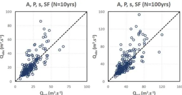
Figure 10.Scatterplot of observed versus estimated discharge val-ues for a combination of catchment area, maximum daily precipita-tion total, average catchment slope, shape factor and curve number forT=10 years (left panel) andT=100 years (right panel).
% RMSE=100· s n
P
i=1(Qobs,i−Qest,i) 2
n n P i=1Qobs,i
n
=100· s
n
P
i=1
Qobs,i−Qest,i2
n
P
i=1 Qobs,i
·√n (13)
% MAE=100· n P i=1|
Qobs,i−Qest,i| n n P i=1
Qobs,i n
=100·
n
P
i=1
Qobs,i−Qest,i
n
P
i=1 Qobs,i
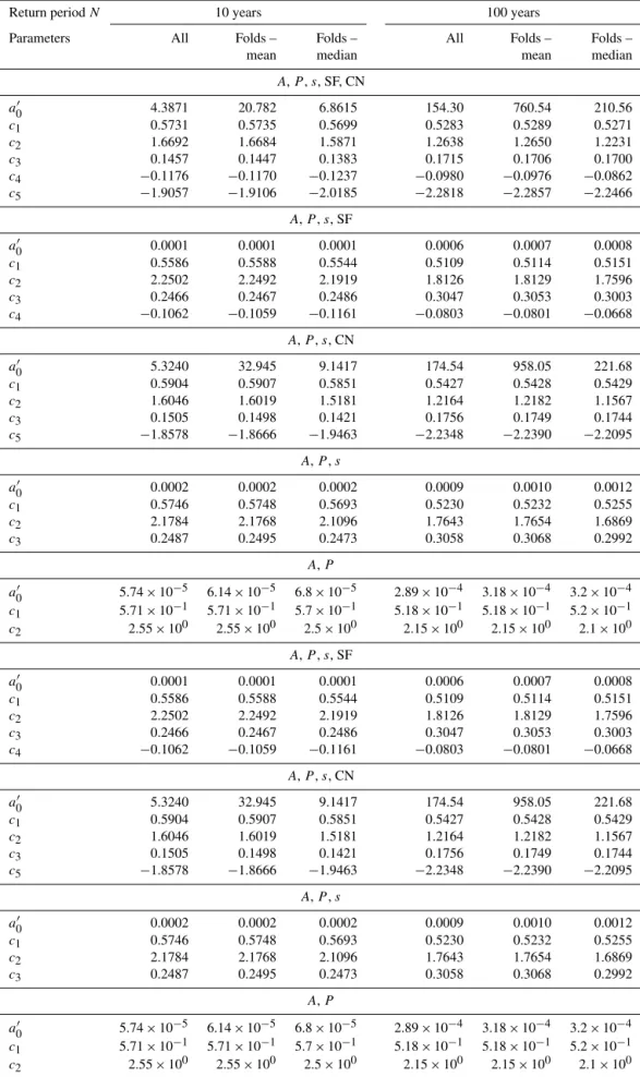
Table 3.Values of calibrated model parameters.
Return periodN 10 years 100 years
Parameters All Folds – Folds – All Folds – Folds –
mean median mean median
A,P,s, SF, CN
a0′ 4.3871 20.782 6.8615 154.30 760.54 210.56
c1 0.5731 0.5735 0.5699 0.5283 0.5289 0.5271
c2 1.6692 1.6684 1.5871 1.2638 1.2650 1.2231
c3 0.1457 0.1447 0.1383 0.1715 0.1706 0.1700
c4 −0.1176 −0.1170 −0.1237 −0.0980 −0.0976 −0.0862
c5 −1.9057 −1.9106 −2.0185 −2.2818 −2.2857 −2.2466
A,P,s, SF
a0′ 0.0001 0.0001 0.0001 0.0006 0.0007 0.0008
c1 0.5586 0.5588 0.5544 0.5109 0.5114 0.5151
c2 2.2502 2.2492 2.1919 1.8126 1.8129 1.7596
c3 0.2466 0.2467 0.2486 0.3047 0.3053 0.3003
c4 −0.1062 −0.1059 −0.1161 −0.0803 −0.0801 −0.0668
A,P,s, CN
a0′ 5.3240 32.945 9.1417 174.54 958.05 221.68
c1 0.5904 0.5907 0.5851 0.5427 0.5428 0.5429
c2 1.6046 1.6019 1.5181 1.2164 1.2182 1.1567
c3 0.1505 0.1498 0.1421 0.1756 0.1749 0.1744
c5 −1.8578 −1.8666 −1.9463 −2.2348 −2.2390 −2.2095
A,P,s
a0′ 0.0002 0.0002 0.0002 0.0009 0.0010 0.0012
c1 0.5746 0.5748 0.5693 0.5230 0.5232 0.5255
c2 2.1784 2.1768 2.1096 1.7643 1.7654 1.6869
c3 0.2487 0.2495 0.2473 0.3058 0.3068 0.2992
A,P
a0′ 5.74×10⁻⁵ 6.14×10⁻⁵ 6.8×10⁻⁵ 2.89×10⁻⁴ 3.18×10⁻⁴ 3.2×10⁻⁴
c1 5.71×10⁻¹ 5.71×10⁻¹ 5.7×10⁻¹ 5.18×10⁻¹ 5.18×10⁻¹ 5.2×10⁻¹
c2 2.55×100 2.55×100 2.5×100 2.15×100 2.15×100 2.1×100
A,P,s, SF
a0′ 0.0001 0.0001 0.0001 0.0006 0.0007 0.0008
c1 0.5586 0.5588 0.5544 0.5109 0.5114 0.5151
c2 2.2502 2.2492 2.1919 1.8126 1.8129 1.7596
c3 0.2466 0.2467 0.2486 0.3047 0.3053 0.3003
c4 −0.1062 −0.1059 −0.1161 −0.0803 −0.0801 −0.0668
A,P,s, CN
a0′ 5.3240 32.945 9.1417 174.54 958.05 221.68
c1 0.5904 0.5907 0.5851 0.5427 0.5428 0.5429
c2 1.6046 1.6019 1.5181 1.2164 1.2182 1.1567
c3 0.1505 0.1498 0.1421 0.1756 0.1749 0.1744
c5 −1.8578 −1.8666 −1.9463 −2.2348 −2.2390 −2.2095
A,P,s
a0′ 0.0002 0.0002 0.0002 0.0009 0.0010 0.0012
c1 0.5746 0.5748 0.5693 0.5230 0.5232 0.5255
c2 2.1784 2.1768 2.1096 1.7643 1.7654 1.6869
c3 0.2487 0.2495 0.2473 0.3058 0.3068 0.2992
A,P
a0′ 5.74×10⁻⁵ 6.14×10⁻⁵ 6.8×10⁻⁵ 2.89×10⁻⁴ 3.18×10⁻⁴ 3.2×10⁻⁴
c1 5.71×10⁻¹ 5.71×10⁻¹ 5.7×10⁻¹ 5.18×10⁻¹ 5.18×10⁻¹ 5.2×10⁻¹
Figure 11.Scatterplot of observed versus estimated discharge val-ues for a combination of catchment area, maximum daily pre-cipitation total, average catchment slope and shape factor for
T =10 years (left panel) andT=100 years (right panel).
Figure 12.Scatterplot of observed versus estimated discharge val-ues for a combination of catchment area, maximum daily pre-cipitation total, average catchment slope and curve number for
T =10 years (left panel) andT=100 years (right panel).
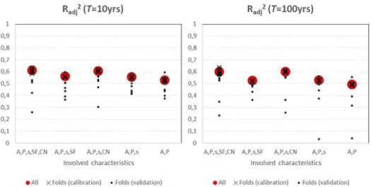
For purposes of validation, values of R2adj were calculated for each fold for both the training and validation set. The comparison with the values obtained by calibration on the whole data set is shown in Fig. 14.
5 Conclusions and outcomes
There are several conclusions that can be drawn based on the performed analyses. First, the influence of each analysed catchment descriptor is not significant enough to be used as the only one explaining peak discharge values. Best re-sults achieve a value of determination coefficient of about R2=0.3. This is not a very strong relationship, and the un-certainty would be too high in the case of considering one single parameter. This outcome was assumed because of the nature of the flood phenomenon. It is a process which is very complex, and there are many factors which play an
Figure 13.Scatterplot of observed versus estimated discharge val-ues for a combination of catchment area, maximum daily precipita-tion total and average catchment slope forT=10 years (left panel) andT =100 years (right panel).
Figure 14.Scatterplot of observed versus estimated discharge val-ues for a combination of catchment area and maximum daily precip-itation total forT=10 years (left panel) andT=100 years (right panel).
important role. Second, the most important catchment de-scriptors are the area and the maximum 24 h precipitation total, which again confirms the initial assumption, although the fit is not as high as expected in the case of the catchment area. Third, the involvement of a land use descriptor (CN) improves the performance of the methodology, even though the initial analysis did not confirm its influence on flood discharges with respect to its definition. Furthermore, this parameter improves the performance even more than shape factor.
Figure 15.Values of the determination coefficient for calibration to the whole data set and for calibration and validation using 7 folds for
T =10 years (left panel) andT=100 years (right panel).
Figure 16.Values of root mean square error (m3s−1) for calibration to the whole data set and for calibration and validation using 7 folds for
T =10 years (left panel) andT=100 years (right panel).
Figure 17.Values of relative root mean square error for calibration to the whole data set and for calibration and validation using 7 folds for
Figure 18.Values of mean absolute error (m3s−1) for calibration to the whole data set and for calibration and validation using 7 folds for
T =10 years (left panel) andT=100 years (right panel).
Figure 19.Values of relative mean absolute error for calibration to the whole data set and for calibration and validation using 7 folds for
T =10 years (left panel) andT=100 years (right panel).
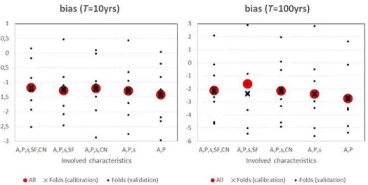
Figure 20.Bias for calibration to the whole data set and for calibration and validation using 7 folds for T=10 years (left panel) and
Figure 21.Values of parameterc1calibrated to the whole data set and to 7 folds forN=10 years (left panel) andN=100 years (right panel).
Figure 22.Values of parameterc2calibrated to the whole data set and to 7 folds forN=10 years (left panel) andN=100 years (right panel).
Figure 23.Values of parameterc3calibrated to the whole data set and to 7 folds forN=10 years (left panel) andN=100 years (right panel).
Figure 25.Values of parameterc5calibrated to the whole data set and to 7 folds forN=10 years (left panel) andN=100 years (right panel).
will need to be done carefully to avoid too high a number of model parameters, which could decrease the robustness. The development will also focus on the possible involvement of soil properties as the characteristic which could improve the performance of the methodology, as it is considered an im-portant factor in flood formation.
The values of RMSE and MAE are shown in Table 1; relative values are then shown in Table 2. The results for calibration using the whole data set show that in the worst case (only area and precipitations are involved), the relative value of RMSE is about 42 %, which is less than the value given by the standard. When all considered catchment de-scriptors are involved, the relative values of RMSE are 38 and 37 % respectively. Scatterplots were drawn for all consid-ered combinations of catchment descriptors to show a fit be-tween observed and estimated values (see Figs. 10–14). The comparison of performance metrics for the calibration us-ing the whole data set and for the calibration usus-ing folds is shown in Figs. 16–19. The values of considered metrics are in general slightly worse than in the case of calibration for the whole data set, but they do not differ much. Calculated bias values show that, in general, the model overestimates flood discharge. Bias values obtained by the calibration for the whole data set and for both training and validation sub-sets are shown in Fig. 20.
Calibrated values of model parameters were compared for the calibration for the whole data set and calibration using folds. These values are shown in Figs. 21–25. The results show that parameter values for folds do not differ much from those obtained by the calibration for the whole data set. In general, the variance of calibrated parameters increases with decreasing importance of the corresponding catchment de-scriptors, being highest in the case of shape factors and curve numbers. The comparison of mean and median values of model parameters obtained for folds with values obtained for the whole data set is provided in Table 3. It shows that both means and medians for folds are very close to values for the whole data set, except for parametera0′. Thus, the fi-nal forms of values obtained for the whole data set and the
Table 4.t values table for considered parameters (tnα/2
−K=1.9723 to 1.9725, forα=0.05,n=196 andK=5 to 2).
Return 10 years 100 years periodT
A,P,s, SF, CN c1 13.3505 12.8022
c2 6.2117 5.7294 c3 2.3224 2.8409 c4 −1.9914 −1.7252
c5 −3.9119 −5.1034
A,P,s, SF
c1 12.5984 11.6803 c2 9.6910 8.8482
c3 4.1603 5.2636 c4 −1.7369 −1.3325
A,P,s, CN
c1 13.9367 13.3565
c2 5.9689 5.5293 c3 2.3822 2.8966
c5 −3.7890 −4.9820
A,P,s
c1 13.1792 12.1989 c2 9.4845 8.7328
c3 4.1738 5.2733 A,P
c1 12.5691 11.3211 c2 11.5528 10.7109
final shape of equations for the calculation of flood discharge values when considering all catchment descriptors except for SF are as shown by Eqs. (14) and (15).
Q100=174.54·A0.5427·P1001.2164·s0.1756·CN−2.2348 (16)
Acknowledgements. The research presented in this paper has
been supported by national grant project COST CZ no. LD11031 “Flood characteristics of small catchments”, which is connected to the international COST Action ES0901 “European procedures for flood frequency estimations”, and by national grant project NAZV KUS no. QJ1220233, “Assessment of former pond systems with aim to achieve sustainable management of water and soil resources in the Czech Republic”. All the support is gratefully acknowledged. The authors would also like to thank the guest editor Thomas R. Kjeldsen and both reviewers for their constructive and useful comments.
Edited by: T. Kjeldsen
Reviewed by: A. Rahman and another anonymous referee
References
Asquith, W. H. and Slade, R. M.: Site-Specific Estimation of Peak-Streamflow Frequency Using Generalized Least Squares Regres-sion for Natural Basins in Texas, USGS, Texas, USA, 1996. Berger, K. P. and Entekhabi, D.: Basin hydrologic response relations
to distributed physiographic descriptors and climate, J. Hydrol., 247, 169–182, 2001.
Burn, D. H.: Catchment similarity for regional flood frequency anal-ysis using seasonality measures, J. Hydrol., 202, 212–230, 1997. David, V.: Catchment shape descriptors as an input to flood hazard classification., in: Proceedings of the 12th International Confer-ence on Environmental SciConfer-ence and Technology, University of the Aegean, Aegean, B.205–B.212, 2011.
Eng, K., Milly, P. C. D., and Tasker, G. D.: Flood regionalization: a hybrid geographic and predictor-variable region-of-influence regression method, J. Hydrol. Eng., 12, 585–591, 2007. Haddad, K. and Rahman, A.: Regional flood frequency analysis
in eastern Australia: Bayesian GLS regression-based methods within fixed region and ROI framework – Quantile Regression vs. Parameter Regression Technique, J. Hydrol., 430–431, 142– 161, 2012.
Haddad, K., Rahman, A., and Stedinger, J.: Regional flood fre-quency analysis using Bayesian generalized least squares: a com-parison between quantile and parameter regression techniques, Hydrol. Process., 26, 1008–1021, 2012.
Haddad, K., Rahman, A., Zaman, M. A., and Shrestha, S.: Applica-bility of Monte Carlo cross validation technique for model devel-opment and validation using generalised least squares regression, J. Hydrol., 482, 119–128, 2013.
Jaafar, W. Z., Liu, J., and Han, D.: Input variable selection for median flood regionalization, Water Resour. Res., 47, W07503, doi:10.1029/2011WR010436, 2011.
Kjeldsen, T. R. and Rosbjerg, D.: Comparison of regional index flood estimation procedures based on the extreme value type I distribution, Stoch. Environ. Res. Risk A., 16, 358–373, 2002. Kulasová, B. and Holík, J.: ˇCSN 75 1400 – Hydrological data on
surface water, Czech Standards Institute, Prague, 1997.
McCuen, R. H., Leahy, R. B., and Johnson, P. A.: Problems with logarithmic transformations in regression, J. Hydraul. Eng., 116, 414–428, 1990.
Merz, R. and Blöschl, G.: Flood frequency regionalisation – spatial proximity vs. catchment attributes. Journal of Hydrology, 302, 283–306, 2005.
Micevski, T. and Kuczera, G.: Combining site and regional flood information using a Bayesian Monte Carlo approach, Water Re-sour. Res., 45, W04405, doi:10.1029/2008WR007173, 2009. Mishra, S. K. and Singh, V. P.: Soil Conservation Service Curve
Number (SCS-CN) Methodology, Kluwer Academic Publishers, Dordrecht, p. 513, 2003.
Murthy, C. S.: Water Resources Engineering: Principles and Prac-tice, New Age International (P) Limited, Delhi, India, p. 314, 2002.
Nezhad, M. K., Chokmani, K., Ouarda, T. B. M. J., Barbet, M., and Bruneau, P.: Regional flood frequency analysis using resid-ual kriging in physiographical space, Hydrol. Process., 24, 2045– 2055, 2010.
Olson, S. A.: Estimation of flood discharges at selected recurrence intervals for streams in New Hampshire, US Geological Survey Scientific Investigations Report 2008-5206, US Geological Sur-vey, Reston, Virginia, USA, 2009.
Padney, G. R.,and Nguyen, V.-T.-V.: A comparative study of regres-sion based methods in regional flood frequency analysis, J. Hy-drol., 225, 92–101, 1999.
Patil, S. and Stieglitz, M.: Controls on hydrologic similarity: role of nearby gauged catchments for prediction at an ungauged catch-ment, Hydrol. Earth Syst. Sci., 16, 551–562, doi:10.5194/hess-16-551-2012, 2012.
Perrin, C., Michel, C., and Andréassian, V.: Does a large number of parameters enhance model performance? Comparative assess-ment of common catchassess-ment model structures on 429 catchassess-ments, J. Hydrol., 242, 275–301, 2001.
Reed, D. W. and Field, E. K.: Reservoir Flood Estimation: Another Look, Wallingford, England, p. 87, 1992.
Šamaj, F., Valoviˇc, Š., and Brázdil, R.: Denné úhrny zrážok s mimo-riadnou výdatnost’ou v ˇCSSR v období 1901–1980, in: Zborník práce Slovenského hydrometeorologického ústavu, ALFA, vyda-vatestvo technickej a ekonomickej literatúry, Bratislava, 1985. Sefton, C. E. M. and Howarth, S. M.: Relationships between
dy-namic response characteristics and descriptors of catchments in England and Wales, J. Hydrol., 211, 1–16, 1998.
Sivapalan, M., Jothityangkoon, C., and Menabde, M.: Linearity and nonlinearity of basin response as a function of scale: Discussion of alternative definitions, Water Resour. Res., 38, 4.1–4.5, 2002. Stedinger, J. R. and Tasker, G. D.: Regional hydrologic analysis, 1. Ordinary, weighted and generalized least squares compared, Water Resour. Res., 21, 1421–1432, 1985.
Wagener, T., Sivapalan, M., Troch, P., and Woods, R.: Catchment classification and hydrologic similarity, Geogr. Compass, 1, 901– 931, doi:10.1111/j.1749-8198.2007.00039.x, 2007.
Willmott, C. J. and Matsuura, K.: Advantages of the mean absolute error (MAE) over the root mean square error (RMSE) in assess-ing average model performance, Clim. Res., 30, 79–82, 2005. Zítek, J. (Ed.): Hydrologické pomˇery ˇCeskoslovenské socialistické