Observation of horizontal winds in the middle-atmosphere between 30° S and 55° N during the northern winter 2009–2010

(1)

ACPD

12, 32473–32513, 2012

SMILES winds

P. Baron et al.

Title Page

Abstract Introduction

Conclusions References

Tables Figures

◭ ◮

Back Close

Full Screen / Esc

Printer-friendly Version Interactive Discussion

Discussion

P

a

per

|

Dis

cussion

P

a

per

|

Discussion

P

a

per

|

Discussio

n

P

a

per

|

Atmos. Chem. Phys. Discuss., 12, 32473–32513, 2012 www.atmos-chem-phys-discuss.net/12/32473/2012/ doi:10.5194/acpd-12-32473-2012

Atmospheric Chemistry and Physics Discussions

This discussion paper is/has been under review for the journal Atmospheric Chemistry and Physics (ACP). Please refer to the corresponding final paper in ACP if available.

Observation of horizontal winds in the

middle-atmosphere between 30

◦

_{S and}

55

◦

_{N during the northern winter}

2009–2010

P. Baron1, D. P. Murtagh2, J. Urban2, H. Sagawa1, S. Ochiai1, H. K ¨ornich3,

F. Khosrawi4, K. Kikuchi1, S. Mizobuchi5, K. Sagi2, Y. Kasai1,6, and M. Yasui1

1

National Institute of Information and Communications Technology, 4-2-1 Nukui-kitamachi, Koganei, Tokyo 184-8795, Japan

2

Department of Earth and Space Science, Chalmers University of Technology, 412 96 G ¨oteborg, Sweden

3

SMHI, Folkborgsv ¨agen 1, 601 76 Norrk ¨oping, Sweden

4

Department of Meteorology University of Stockholm 10691 Stockholm, Sweden

5

Japan Aerospace Exploration Agency, Tsukuba, 305-8505 Japan

6

(2)

ACPD

12, 32473–32513, 2012

SMILES winds

P. Baron et al.

Title Page

Tables Figures

◭ ◮

Back Close

Full Screen / Esc

Discussion

P

a

per

|

Dis

cussion

P

a

per

|

Discussion

P

a

per

|

Discussio

n

P

a

per

|

Received: 17 October 2012 – Accepted: 10 December 2012 – Published: 17 December 2012

Correspondence to: P. Baron (baron@nict.go.jp)

(3)

ACPD

12, 32473–32513, 2012

SMILES winds

P. Baron et al.

Title Page

Tables Figures

◭ ◮

Back Close

Full Screen / Esc

Discussion

P

a

per

|

Dis

cussion

P

a

per

|

Discussion

P

a

per

|

Discussio

n

P

a

per

|

Abstract

Although the links between stratospheric dynamics, climate and weather have been demonstrated, direct observations of stratospheric winds are lacking. We report

obser-vations of winds between 8 and 0.01 hPa (∼35–80 km) from October 2009 to April 2010

by the Superconducting Submillimeter-Wave Limb-Emission Sounder (SMILES) on the

5

International Space Station. The altitude range covers the region between 35–60 km where previous space-borne wind instruments show a lack of sensitivity. Both zonal and meridional wind components were obtained, though not simultaneously, in the

lati-tude range from 30◦S to 55◦N and with a single profile precision of 7–9 m s−1between

8 and 0.6 hPa and better than 20 m s−1 at altitudes above. The vertical resolution is

10

5–7 km except in the upper part of the retrieval range (10 km at 0.01 hPa). In the region

between 1–0.05 hPa, a mean difference <2 m s−1 is found between SMILES profiles

retrieved from different spectroscopic lines and instrumental settings. Good agreement

(mean di_fference of ∼2 m s−1) is also found with the European Centre for

Medium-Range Weather Forecasts (ECMWF) analysis in most of the stratosphere except for

15

the zonal winds over the equator (mean difference of 5–10 m s−1). In the mesosphere,

SMILES and ECMWF zonal winds exhibit large di_fferences (>20 m s−1_{), especially in}

the tropics. We illustrate our results by showing daily and monthly zonal wind variations, namely the semi-annual oscillation in the tropics and reversals of the flow direction

between 50◦_N–55◦_{N during sudden stratospheric warmings in the stratosphere. The}

20

daily comparison with ECMWF winds reveals that in the beginning of February, a sig-nificantly stronger zonal westward flow is measured in the tropics at 2 hPa compared to

the flow computed in the analysis (di_fference of∼20 m s−1). The results show that the

comparison between SMILES and ECMWF winds is not only relevant for the quality assessment of the new SMILES winds but it also provides insights on the quality of the

25

(4)

ACPD

12, 32473–32513, 2012

SMILES winds

P. Baron et al.

Title Page

Tables Figures

◭ ◮

Back Close

Full Screen / Esc

Discussion

P

a

per

|

Dis

cussion

P

a

per

|

Discussion

P

a

per

|

Discussio

n

P

a

per

|

have the potential to provide good quality data for improving the stratospheric winds in atmospheric models.

1 Introduction

Stratospheric winds play an important role in stratospheric chemistry by transporting long-lived species, or by creating transport barriers that for example isolate the

po-5

lar vortex in winter (Shepherd, 2007, 2008). The stratospheric Quasi-biennial Oscil-lation (QBO) and downward feedback from the stratospheric vortex to tropospheric weather systems have also been reported to be relevant both in the context of weather prediction and climate (Baldwin and Dunkerton, 1999; Baldwin et al., 2003; Sigmond et al., 2008; Marshall and Scaife, 2009; Wang and Chen, 2010). In addition,

strato-10

spheric winds describe and a_ffect vertically propagating atmospheric waves that control

the transport circulation in the stratosphere and mesosphere (Holton and Alexander, 2000).

In meteorological analyses and reanalyses, unobserved variables are constrained by observed ones through the use of balance relationships. The application of a

mass-15

wind balance (Derber and Bouttier, 1999) leads to a state where the large number of temperature soundings provide a strong constraint on the balanced wind compo-nent, i.e. approximately the geostrophic wind. However, this balance is not valid for non-geostrophic motion such as equatorial waves (Hamilton, 1998; ˇZagar et al., 2004) or for the middle atmospheric transport circulation (Polavarapu et al., 2005). A further

20

complication in the middle atmosphere is that the small errors from the lower atmo-sphere propagate vertically and amplify strongly in the upper stratoatmo-sphere and meso-sphere (Nezlin et al., 2009; Alexander et al., 2010). Thus, in order to constrain middle atmospheric winds in meteorological analyses, global wind observations in the mid-dle atmosphere are essential. Lahoz et al. (2005) have shown that wind observations

25

(5)

ACPD

12, 32473–32513, 2012

SMILES winds

P. Baron et al.

Title Page

Tables Figures

◭ ◮

Back Close

Full Screen / Esc

Discussion

P

a

per

|

Dis

cussion

P

a

per

|

Discussion

P

a

per

|

Discussio

n

P

a

per

|

significant improvements of zonal-winds analyses especially in the tropical middle and upper stratosphere (50–1 hPa).

In spite of the importance of middle atmospheric observations, wind measurements assimilated in the models are mostly limited to the troposphere. In the mesosphere, winds are measured using optical techniques from satellites (Shepherd et al., 1993;

5

Hays et al., 1993; Killeen et al., 1999; Swinbank and Ortland, 2003; Niciejewski et al., 2006) and by ground-based radar systems such as European Incoherent SCATter (EISCAT) (Alcayd ´e and Fontanari, 1986) and various meteor radars (Maekawa et al., 1993; Jacobi et al., 2009). Wu et al. (2008) have used the microwave oxygen line at 118 GHz measured by the Microwave Limb Sounder (MLS) to derive line-of-sight winds

10

in the mesosphere (80–92 km). The authors suggested that winds can be derived down to 40 km by using emission lines from other molecules, but no results have been shown yet. Stratospheric winds have been measured from the ground using active and pas-sive techniques (Hildebrand et al., 2012; R ¨ufenacht et al., 2012) and from space by the

High Resolution Doppler Imager (HRDI) on UARS covering 10–35 km and 60◦S–60◦N,

15

using the molecular oxygen A- and B-bands (Ortland et al., 1996).

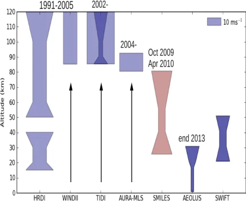
Figure 1 summarises previous and planned wind measuring instruments from

space-borne platforms. A gap in the coverage of high quality winds (<5 m s−1error) between

30 and 60 km clearly exists. The ESA Atmospheric Dynamics Mission on the Aeolus

satellite is planned for 2013–2014 (Stoffelen et al., 2005) for measuring winds in the

tro-20

posphere and lower stratosphere using a IR/UV lidar. For middle-stratospheric winds, the Stratospheric Wind Interferometer For Transport studies (SWIFT) instrument was planned by the Space Canadian Agency for 2010 (McDade et al., 2001) but has an unclear future at the time of writing. The target of SWIFT is to measure the thermal

emission from O3lines at at 8 µm in order to provide winds on a near global scale

be-25

tween 15–50 km with the best accuracy of 3–5 m s−1_{between 20–40 km and a vertical}

resolution of 2 km.

(6)

ACPD

12, 32473–32513, 2012

SMILES winds

P. Baron et al.

Title Page

Tables Figures

◭ ◮

Back Close

Full Screen / Esc

Discussion

P

a

per

|

Dis

cussion

P

a

per

|

Discussion

P

a

per

|

Discussio

n

P

a

per

|

(SMILES) onboard the Japanese Experiment Module (JEM) of the International Space Station (ISS) (Kikuchi et al., 2010; Ochiai et al., 2012b). The instrument was launched in September 2009 for deriving trace gas profiles. Although SMILES was not designed for this purpose, we have exploited its high frequency resolution and high signal to noise ratio to derive the small Doppler shifts in the atmospheric spectra and thereby

5

line-of-sight wind velocities. Because of the ISS rotation during an orbit, both zonal and

meridional components (±10◦) are retrieved between 30◦S–55◦N. As shown in this

analysis, the wind information is derived from 8–0.01 hPa (∼35–80 km) with a

preci-sion better than 10 m s−1 at altitudes between 6 and 0.5 hPa and better than 20 m s−1

at altitudes above.

10

The main purpose of this paper is to present the wind data that has been derived from the six months of SMILES observations (October 2009 to April 2010) as well as assessing its quality. A further purpose is to compare the SMILES measurements with the operational winds analysis by the European Centre for Medium-Range Weather Forecasts (ECMWF). At mid-latitude in the mid-stratosphere, ECMWF winds are

ex-15

pected to be reliable and to provide a good data set to check the SMILES wind quality. On the other hand, ECMWF results are uncertain in the mid- and high stratosphere of the tropical region. Because of the lack of other stratospheric wind measurements,

SMILES data offer a unique opportunity to estimate the performances of the ECMWF

wind analyses in this region.

20

In Sect. 2, we briefly describe the measurement method. The theoretical precision (random errors) and accuracy (systematic errors) are estimated from a sensitivity study. Section 3 assesses the quality of the SMILES data by checking the internal

consis-tency of the different SMILES products. The mean differences with the ECMWF winds

are discussed. Results are illustrated with monthly global maps and the daily

varia-25

tion of the zonal-winds in Sect. 4. Both the measured Semi-Annual Oscillations (SAO)

of the zonal-wind above the Equator, and the zonal-wind reversals between 50◦N–

(7)

ACPD

12, 32473–32513, 2012

SMILES winds

P. Baron et al.

Title Page

Tables Figures

◭ ◮

Back Close

Full Screen / Esc

Discussion

P

a

per

|

Dis

cussion

P

a

per

|

Discussion

P

a

per

|

Discussio

n

P

a

per

|

are compared with the ECMWF analysis. Finally, we summarise our results and give conclusions as well as discuss ongoing work for improving the SMILES wind products.

2 SMILES observations

2.1 Measurement method

SMILES was attached to the ISS in Sept 2009 and functioned for 7 months

un-5

til April 2010. It observed the Earth’s limb, scanning from −7 to 100 km in 53 s,

providing 1600 spectral radiance profiles per day. Using superconductor-Insulator-superconductor (SIS) detectors cooled at 4 K, it provided high quality spectra allowing

constituent profiles of many species such as ozone (O₃) and hydrogen chloride (HCl) to

be derived (Kasai et al., 2006; Takahashi et al., 2010; Khosravi et al., 2012). SMILES

10

observed spectral lines from the atmospheric limb in three frequency bands, named A (624.3–625.5 GHz), B (625.1–626.3 GHz) and C (649.1–650.3 GHz) but only two are measured simultaneously. Two acousto-optical spectrometers (AOS-1 and AOS-2) with similar specifications are used. Frequency calibration and stability are ensured using an ultra-stable oscillator and frequent comb calibration of the AOS (Mizobuchi et al.,

15

2012). Inherent in the spectra is information on the Doppler shift caused by the ISS

(∼4 km s−1 along the line of sight) as well as atmospheric motion. The broadening

of the spectral lines into several spectral channels provides enough sensitivity to

de-tect the small frequency shift induced by the winds (e.g. a 50 m s−1 line-of-sight wind

induced a shift of 100 kHz which has to be compared to the spectrometer spectral

res-20

olution of 1.2 MHz). For deriving wind, the two strongest spectral lines have been used

separately. One is an emission line of O3 at 625.371 GHz common to bands A and B,

and the second one is a H35Cl triplet at 625.92 GHz (band B). Hence, three winds

pro-files are independently retrieved, two from the O₃line in bands A and B, and one from

the HCl triplet in band B. The wind retrieval algorithm is similar to the one presented in

25

(8)

ACPD

12, 32473–32513, 2012

SMILES winds

P. Baron et al.

Title Page

Tables Figures

◭ ◮

Back Close

Full Screen / Esc

Discussion

P

a

per

|

Dis

cussion

P

a

per

|

Discussion

P

a

per

|

Discussio

n

P

a

per

|

more details). The retrieved wind profiles are corrected to take into account the altitude dependence of the line-of-sight velocity which is neglected in the trace gas retrieval

algorithms (∼0.8 m s−1km−1).

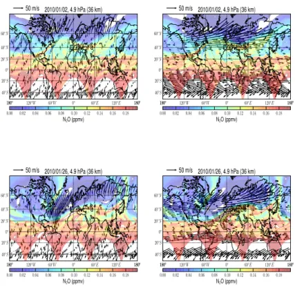
Because of the geometry of the instrument field of view in relation to the ISS orbit,

the meridional component (±10◦) of the wind is measured on the ascending portion of

5

the orbit while the zonal component is measured on the descending portion. Figure 2 shows single line-of-sight wind retrievals at 36 km on 2 and 26 January for both ascend-ing and descendascend-ing portions of the orbits. Winds are retrieved near the meridional or

the zonal directions between∼30◦S to∼55◦N. The full latitude range of observations

is between 38◦S and 65◦N but on the borders, the line-of-sight rotates quickly and

de-10

viates from the meridional or zonal direction. Another characteristic of the observations is, as the result of the 2-months periodic local-time precession of the ISS, semi and diurnal variations of mesospheric winds such as those induced by tides should have been captured in the observations.

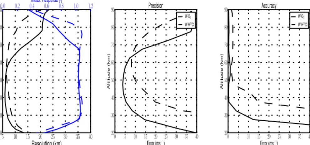
2.2 Theoretical estimation of the retrieval errors

15

Figure 3 (left panel) shows the vertical resolution of the retrieved wind profiles and the measurement responses that indicate the altitudes of good measurement sensi-tivity (Merino et al., 2002). Considering altitudes where the measurement response is between 0.9–1.1, a good sensitivity is found from 25 to 70 km (20–0.05 hPa) and from

25 to 80 km (20–0.01 hPa) for the O3and HCl line retrievals, respectively. According to

20

the vertical resolution of the retrieved profiles, the best information is obtained from the

O3 line below 60 km (0.2 hPa), and from the HCl lines at altitudes above. The vertical

resolution of the composite retrieved profile is 5–7 km up to 70 km and increases to 10 km at 80 km. Since the wind information comes from a layer of 5 to 10 km thickness around the line-of-sight tangent point, the horizontal resolution along the line-of-sight

25

is between 500 and 700 km.

(9)

ACPD

12, 32473–32513, 2012

SMILES winds

P. Baron et al.

Title Page

Tables Figures

◭ ◮

Back Close

Full Screen / Esc

Discussion

P

a

per

|

Dis

cussion

P

a

per

|

Discussion

P

a

per

|

Discussio

n

P

a

per

|

of the error analysis are given in Baron et al. (2011), except for the errors on the cali-bration parameters which include a correction for a non-linearity in the receiver (Ochiai et al., 2012a). Here an error of 20 % is assumed on the non-linear parameters. The retrieval precision is limited by the measurement noise and to a lesser extent by the

uncertainties in the O₃ and HCl abundances. The theoretical precision is 4–10 m s−1

5

between 35 and 60 km (O3 line retrieval) and<20 m s−

1

between 60 and 80 km (HCl

line retrieval). The lower limit of accurate retrieval is set by systematic effects on the

ozone line retrieval (dashed black line), in particular errors on the intensity calibration of the spectra.

In summary, although the retrieval sensitivity reaches down to 25 km, good quality

10

wind profiles (accuracy<5 m s−1

) are actually retrieved from 35 km (8 hPa). The upper limit of the retrieval is 80 km using the band-B HCl line.

2.3 Data selection and ECMWF wind pairing

In this analysis, retrieved winds with a measurement response smaller than 0.9 are rejected. The retrieval quality is estimated from the sum of the squares of the spectral

15

fit residual (χ2). Abnormally high values of the χ2 before the retrieval indicate scans

with potential disturbances in the field-of-view or in the pointing. High values of the

χ2 after the retrieval indicates bad measurement fit. Note that disturbed observations

can be fitted effectively but with incorrect wind values. Hence it is important to test the

χ2 before and after the retrieval. For the O3 line in band-A (band-B), retrievals with

20

a normalizedχ2larger than 40 (30) before the inversion or larger than 2 (1.5) after the

inversion are rejected. For the HCl line in band-B, theχ2thresholds for rejection are 50

before inversion and 2.5 after inversion.

ECMWF operational analysis data were used starting with Integrated Forecasting system (IFS) cycle 35 release 3 in September 2009. A major operational upgrade

oc-25

(10)

ACPD

12, 32473–32513, 2012

SMILES winds

P. Baron et al.

Title Page

Tables Figures

◭ ◮

Back Close

Full Screen / Esc

Discussion

P

a

per

|

Dis

cussion

P

a

per

|

Discussion

P

a

per

|

Discussio

n

P

a

per

|

to 16 km. To compare the measurements with the ECMWF analysis, the SMILES pro-files are paired with the closest ECMWF profile in space and time. ECMWF analyses

were extracted on a latitude-longitude grid of 0.5×0.5◦and 4 times per day, which

cor-responds to coincidence criteria of 3 h and 0.25◦. The profiles extend up to 0.01 hPa

(∼80 km) with a vertical resolution of about 1.5 km in the middle stratosphere. The

5

component of the ECMWF winds parallel to the SMILES line-of-sight is computed with the vertical resolution degraded to that of the retrieved profiles based on the shape of the retrieval averaging kernels.

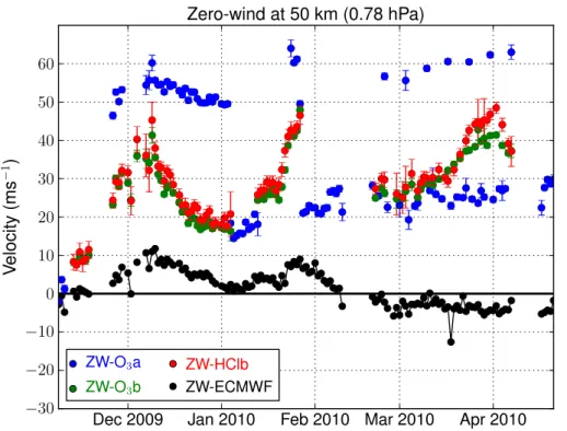
2.4 Zero-wind correction

Errors which are not significant for trace gas retrieval, have not been fully characterized

10

properly and were not included in the error analysis described in Sect. 2.2. However, wind retrievals are sensitive to some of these errors such as the spectrometer fre-quency calibration, the main local-oscillator frefre-quency, the line-of-sight velocity correc-tion and knowledge of the spectroscopic line frequency. The systematic component of these errors is mitigated by subtracting a daily “zero-wind” profile consisting of the

aver-15

age of observations with a direction near the meridional direction (±10◦) and located in

the tropics (±20◦from the equator) where the actual flow is predominantly zonal. Note

that the latitude range of±20◦has been defined to minimize the atmospheric

contribu-tion in the zero-wind based on estimacontribu-tions using the ECMWF winds. Figure 4 shows the zero-winds at 50 km derived from the three SMILES products. At this altitude, the

20

three products are retrieved with a good sensitivity and the spectrometer frequency error is expected to be the main measurement bias. For lines in band-B, which is al-ways measured with the second spectrometer unit (AOS-2), the zero-wind corrections

vary between 20–40 m s−1

and the day-to-day changes do not exceed 5 m s−1

. The

zero-wind correction retrieved from the O3line in band-A shows two regimes

depend-25

ing which spectrometer is used. When the first spectrometer unit (AOS-1) is used for the measurements (configuration for measuring band-B simultaneously), the zero-wind

(11)

ACPD

12, 32473–32513, 2012

SMILES winds

P. Baron et al.

Title Page

Tables Figures

◭ ◮

Back Close

Full Screen / Esc

Discussion

P

a

per

|

Dis

cussion

P

a

per

|

Discussion

P

a

per

|

Discussio

n

P

a

per

|

zero-wind values are similar to those obtained for band-B. After removing the atmo-spheric wind variability estimated using ECMWF winds (ECMWF zero-wind in Fig. 4),

a linear trend of∼20 m s−1/6-months is seen on the 4 observational configurations (not

shown). This trend is compatible with the main local-oscillator stability expected to be δν

ν =6.8×10

−8

/6-months whereνis the local oscillator frequency. Zero-wind corrections

5

relevant to band B oscillate with a period of 2-months and an amplitude of 10–20 m s−1_.

Although the period is compatible with that of the instrument thermal variation, the ori-gin of the oscillation on the band-B zero-wind is not yet fully understood.

Such frequency offsets (<0.1 MHz) are acceptable for trace gas retrievals which are

the first objective of the mission. However it is clearly not good enough for wind retrieval

10

which requires the “zero-wind” correction. However, as seen by the ECMWF zero-wind, during some periods between December and February the atmospheric contribution

in the zero-wind correction can reach∼10 m s−1 which would introduce a bias in the

wind profile if solely corrected with the retrieved zero-wind value. In order to reduce this bias, the subtraction of the retrieved zero-wind is compensated by the addition of

15

ECMWF zero-wind. Above 0.01 hPa, ECMWF winds are not available and are linearly extrapolated.

3 Data quality assessment and comparison with ECMWF analysis

The data quality assessment consists, first, of checking the internal consistency of the

SMILES data since winds are derived from different spectroscopic lines and

spectrom-20

eters. For further verification, retrieved winds need to be compared with independent wind information. Lacking other measurements in the middle and upper stratosphere, such information is taken from the operational ECMWF analyses. It is known that, at high altitudes, tropical ECMWF winds are poorly constrained. Baldwin and Gray (2005) have compared ECMWF ERA-40 reanalysis zonal-winds with observations from two

25

(12)

ACPD

12, 32473–32513, 2012

SMILES winds

P. Baron et al.

Title Page

Tables Figures

◭ ◮

Back Close

Full Screen / Esc

Discussion

P

a

per

|

Dis

cussion

P

a

per

|

Discussion

P

a

per

|

Discussio

n

P

a

per

|

of 0.3 at 0.1 hPa with observations). Hence, the comparison of SMILES with ECMWF winds is not only relevant for the SMILES wind quality assessment but it also provides insights on the quality of the ECMWF winds themselves. For full verification of the SMILES winds, the mesospheric measurements should also be validated with ground-based radar observations. However such analysis is beyond the scope of this paper.

5

3.1 Internal consistency check

The upper panels of Fig. 5 show the mean meridional wind profiles in 20◦latitude bins

between 20◦S and 60◦N that have been retrieved from the O3 lines in bands A and

B (blue and green lines, respectively) and from the HCl line in band B (red line). Only measurements when bands A and B were measured simultaneously are used. The

10

retrieved winds have been corrected with the zero-wind profile.

Between 4 and 0.1 hPa, good agreement is found for winds retrieved from the O₃

lines in all latitude bands. The standard deviation of the retrieved winds (Fig. 5, lower

panels) also confirms the good agreement between the O3 retrievals in this altitude

range. At lower (8–4 hPa) and upper (<0.1 hPa) altitudes, O₃line derived winds exhibit

15

differences that reach∼10 m s−1at higher latitudes.

As indicated in Sect. 2.2, in the upper retrieval range (0.1–0.01 hPa), winds retrieved from the HCl line should be preferred. Between 1 and 0.1 hPa, the mean and the stan-dard deviation of the profiles retrieved from the HCl line (dashed-red line) match those

from the O3retrievals. At higher altitudes, the mean and standard deviation of the HCl

20

wind profiles smoothly expands up to 0.005 hPa. In the lower part of the retrieval range

(>1 hPa), large differences with O3retrievals can be seen as expected from the

degra-dation of the accuracy and the precision of the HCl line retrieval.

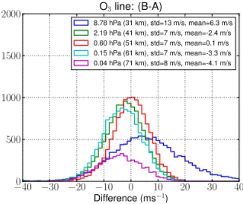
The left panel of Fig. 6 shows the differences between profiles retrieved from the O₃

and the HCl lines in band-B between 40 and 70 km. At 50 and 60 km, the standard

devi-25

ation and the mean of the differences are 12 m s−1and<1.2 m s−1, respectively. Since

(13)

ACPD

12, 32473–32513, 2012

SMILES winds

P. Baron et al.

Title Page

Tables Figures

◭ ◮

Back Close

Full Screen / Esc

Discussion

P

a

per

|

Dis

cussion

P

a

per

|

Discussion

P

a

per

|

Discussio

n

P

a

per

|

thermal noise. The value is consistent with the theoretical estimate: 5–8 m s−1 and

10 m s−1 for O3 and HCl retrievals, respectively. At 70 km, the standard deviation

in-creases to 16 m s−1 which is also consistent with the loss of precision for both O3and

HCl retrievals (20 m s−1 and 13 m s−1, respectively). The slight overestimation of the

O₃-line retrieval precision is because of the large variability of the mesospheric O₃line

5

intensity in the mesosphere.

The comparison of the winds derived from the ozone line simultaneously measured

in bands A and B (different spectrometers) and corrected with the zero-wind technique

is shown in Fig. 6 (right panel). The mean difference at altitudes between 40–60 km is

less than 3 m s−1and the standard deviation of the differences is 7 m s−1. At 30 km, the

10

mean difference and the standard deviation increase to 6 m s−1and 13 m s−1,

respec-tively. Since the profiles are retrieved from the same spectral line, the measurement

thermal noise is correlated at more than 90 % and the differences between the

re-trievals arise from errors on the spectrometer channels frequency. We checked that

the difference is random from one retrieval to another. Hence, the residual errors from

15

the spectrometer channels frequency after the zero wind correction can be assumed

as a random retrieval error of∼5–7 m s−1.

In conclusion, the di_fferent SMILES products agree with each other in the mid- and

upper stratosphere where the retrieval performances are similar for each product. Our

results also confirm that winds retrieved from the O3 line should be used between

20

8–0.1 hPa while those obtained from the HCl line retrievals should be used between 0.1–0.01 hPa. The theoretical estimate of the retrieval precision is underestimated by

5 m s−1due to a residual error after the zero-wind correction. The additional noise likely

arises from the fluctuation in the spectrometer frequency errors. Taking into account

this additional noise, the total precision of the wind retrieval becomes 7–9 m s−1in the

25

(14)

ACPD

12, 32473–32513, 2012

SMILES winds

P. Baron et al.

Title Page

Tables Figures

◭ ◮

Back Close

Full Screen / Esc

Discussion

P

a

per

|

Dis

cussion

P

a

per

|

Discussion

P

a

per

|

Discussio

n

P

a

per

|

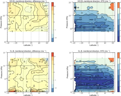
3.2 Comparison with the ECMWF meridional component

The internal checks presented in the previous section do not allow us to estimate the impacts of errors of the platform line-of-sight velocity, and of the local-oscillator

fre-quency, which affect the three wind products in the same way. However in the tropics

and extra-tropical stratosphere where meridional velocities are weak (Fig. 5), the diff

er-5

ences between ECMWF and SMILES single profiles are caused by the retrieval errors, and, to a lesser extent, by non-coincident and non-simultaneous profile pairing and

by uncertainties of ECMWF analysis. Hence the analysis of the differences between

SMILES and ECMWF meridional winds in the stratosphere allows us to verify the wind retrieval error estimations.

10

The mean and the standard deviation of the differences (SMILES-ECMWF) have

been calculated in latitude bins of 5◦for data between November 2009 and April 2010,

and with a line-of-sight within ±10◦ around the meridional direction. We rejected the

days when less than 10 profiles were used to construct the zero-wind profile. Fig. 7

(lower panels) shows the results for the data retrieved from the O3line in band B. Over

15

most of the region between 5–0.5 hPa, the bias between the model and the

measure-ment (left panel) is less than 2 m s−1 and the standard deviation (right panel) is less

than 10 m s−1. However, the bias in the tropics is not relevant since the zero-wind

cor-rection is scaled according to the mean ECMWF tropical meridional wind. According to these results, the precision (standard deviation) and the accuracy (bias) for a single

20

retrieved profile cannot exceed 10 m s−1 and 2 m s−1, respectively, which is consistent

with the error estimation.

At high latitudes (40◦N–60◦N), a mean difference of 2–5 m s−1 is found at 4–3 hPa

which may arise from the increase of the measurement bias and also from the larger

variability of the meridional winds (Fig. 5). At lower altitudes (>8 hPa) and outside the

25

tropics, the large mean differences are due to measurement calibration errors. The

calibration errors are found to be larger for the O3line band-A retrieval (not shown). In

(15)

ACPD

12, 32473–32513, 2012

SMILES winds

P. Baron et al.

Title Page

Tables Figures

◭ ◮

Back Close

Full Screen / Esc

Discussion

P

a

per

|

Dis

cussion

P

a

per

|

Discussion

P

a

per

|

Discussio

n

P

a

per

|

look very similar and are consistent with the decrease of the estimated measurement

precision (between 13 and 20 m s−1

). The mean di_fferences in the mesosphere vary

between−5 and 10 m s−1.

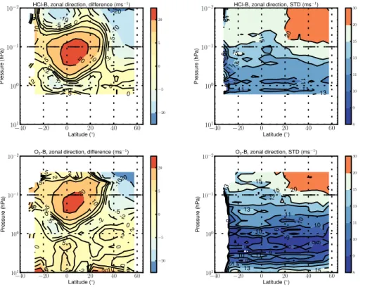
3.3 Comparison with the ECMWF zonal component

In Fig. 8, the same methodology as the previous section is applied for deriving the

5

mean and standard deviation of differences between SMILES (band-B) and ECMWF

zonal (±10◦) winds. Zonal winds are in general significantly larger than the meridional

ones, and thus, the results are more sensitive to mismatches due to profile pairing and ECMWF uncertainties.

As for the meridional component, large mean differences, likely due to intensity

cali-10

bration errors, are found at lower altitudes (>8 hPa) in the extra-tropical regions (lower

right panel) and at latitudes<30◦_{S because of the fast rotation of the line-of-sight from}

the zonal to meridional direction. However in most of the stratosphere (4–1 hPa), a low

bias<2 m s−1is found except over the Equator where the mean difference is between

5–10 m s−1_{. In the mesosphere (1–0.01 hPa, upper right panel), a large positive di}

ff

er-15

ence (20–30 m s−1) is found in the tropics and a negative difference at higher northern

latitudes (between−20 and−10 m s−1).

The standard deviations from the middle-stratosphere to lower mesosphere (lower right panel) are slightly higher than the values found for the meridional components. Such an increase of the standard deviation is consistent with the increase of

uncer-20

tainties in profile-pairing and in ECMWF winds. However, values below 10 m s−1 _are

still found over wide regions and more particularly in the extra-tropics indicating that

SMILES captured the large variations of the zonal winds (−70 to+70 m s−1) with a

pre-cision which is consistent with the estimation of 7–9 m s−1_{. In the tropical mesosphere}

(0.1–0.01 hPa, upper panels), the standard deviation is between 15 and 20 m s−1which

25

also corresponds to the retrieval precision. At northern mid-latitudes, the mesospheric

standard deviation significantly increases to 20–30 m s−1_{, likely due to the increase of}

(16)

ACPD

12, 32473–32513, 2012

SMILES winds

P. Baron et al.

Title Page

Tables Figures

◭ ◮

Back Close

Full Screen / Esc

Discussion

P

a

per

|

Dis

cussion

P

a

per

|

Discussion

P

a

per

|

Discussio

n

P

a

per

|

The comparisons of the meridional and zonal winds derived from SMILES with those from ECMWF are a further indication of the quality of the measurements and of the

retrieval process. The large differences in the zonal-winds found in the tropics and in

the mesosphere indicate that SMILES observations have enough sensitivity to improve the ECMWF zonal wind analyses where the geostrophic approximation is not satisfied.

5

4 Examples of the observed wind fields

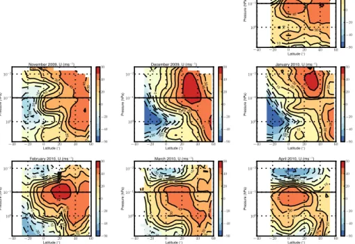
4.1 Monthly variation of zonal-winds

Figure 9 shows the zonally and monthly averaged zonal-winds obtained from band-B

between 30◦_S–55◦_{N and from mid-October to mid-April. Information at lower altitudes}

>0.1 hPa (<65 km) is retrieved from the O3 line and that for the upper altitudes is

10

from the HCl triplet. Until the first week of November, ECMWF were not available to us and the zero-wind correction has been calculated with winds from the version 5.2 of the analysis of the Goddard Earth Observing System Data Assimilation System model (GEOS-5.2) (Reinecker, 2008). In November and February, the observation range

ex-pands poleward in the Southern Hemisphere because of the 180◦_{–maneuver of the ISS}

15

when hosting the space shuttle. The space shuttle also docked in April, but the view-ing geometry did not allow the construction of “zero-wind” profiles. Since the Southern Hemisphere observations corresponded only to a few days, it has been decided to only

focus on the region observed in the normal operation mode (30◦S–55◦N).

The monthly climatology exhibits the main and well known characteristics of the

sea-20

sonal variations of the zonal-winds. Near the equinoxes (October, March and April), in the stratosphere and the lower mesosphere, zonal-winds are primarily eastward. In December and January, they become stronger with a large inter-hemispheric contrast: eastward in the winter-time Northern Hemisphere and westward in the summer-time Southern Hemisphere.

(17)

ACPD

12, 32473–32513, 2012

SMILES winds

P. Baron et al.

Title Page

Tables Figures

◭ ◮

Back Close

Full Screen / Esc

Discussion

P

a

per

|

Dis

cussion

P

a

per

|

Discussion

P

a

per

|

Discussio

n

P

a

per

|

In the tropical upper-stratosphere and mesosphere (<3 hPa), the main

characteris-tics of the Semi-Annual-Oscillation (SAO) in the zonal-winds are seen with, in particular, the opposite phase between the stratosphere (westward in December) and the

meso-sphere (eastward in December). At lower altitudes (>4 hPa), the SAO signal vanishes

and is dominated by the the Quasi-Biennal Oscillation (QBO) which is in an easterly

5

phase (westward winds) during that period. The observed tropical SAO is discussed in more details in Sect. 4.3.

Though the Arctic region is not observed by SMILES, the zonal winds in the

northern-most mid-latitudes (45◦N–55◦N) are influenced by the Arctic polar vortex (high

wester-lies) whose the southerly extent increases with altitude up to the stratopause (∼1 hPa),

10

e.g. in December and January. The dynamics of the Arctic winter 2009/2010 have been described in several studies (Wang and Chen, 2010; D ¨ornbrack et al., 2012; Kuttippu-rath and Nikulin, 2012). In early winter, planetary wave activity prevented the formation of a strong vortex in the lower stratosphere and the vortex eventually split at the begin-ning of December (minor stratospheric warming). From December onward, the vortex

15

became strong throughout the stratosphere until a major sudden stratospheric warm-ing (SSW) occurred on 24–26 January 2010. After this event, a weak vortex reformed

and disappeared in April. It is shown in Sect. 4.2 that the effects of the two SSW are

ob-served at 2 hPa in the daily variation of the mean zonal-wind between 50◦N and 55◦N.

Hence, SMILES offers direct wind measurements for studying the SSW development

20

from the mid-stratosphere (8 hPa) to the mesosphere as well as the interactions with the mid-latitudes.

4.2 The sudden stratospheric warming events

The effects of the major SSW at ∼5 hPa (∼36 km) are clearly seen in Fig. 2. The

coloured background indicates the abundance of N2O from a dynamical model driven

25

by ECMWF winds on the 850 K surface and constrained by Odin/SMR

observa-tions (R ¨osevall et al., 2007). The polar vortex is characterised by low values of N₂O

(18)

ACPD

12, 32473–32513, 2012

SMILES winds

P. Baron et al.

Title Page

Tables Figures

◭ ◮

Back Close

Full Screen / Esc

Discussion

P

a

per

|

Dis

cussion

P

a

per

|

Discussion

P

a

per

|

Discussio

n

P

a

per

|

2010, the vortex is well centered above the polar region and strong eastward winds are measured on its periphery. The direction of the meridional component is alternatively southward or northward following the vortex meanders. On 26 January, the vortex is

displaced over the North of Europe and it is confined between 60◦W and 120◦E.

In-side the vortex, SMILES observed the change of the direction of the meridional winds

5

due to the counterclockwise rotation of the flow. Outside the vortex a westward flow is measured due to an anti-cyclonic system located above the pacific.

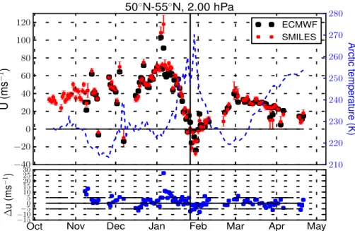
Figure 10 (red dots) shows the daily variation at∼2 hPa of zonally averaged

zonal-winds measured between 50◦N–55◦N. The time series is made from the O3 line

re-trievals. When both bands A and B are measured simultaneously, only band-B is used.

10

The error bars correspond to the daily-mean precision ¯e(2-σ):

¯

e₌ s

e2

n_zero+

e2₊_e2

s

n_wind , (1)

where e₌5 m s−1 is the single profile retrieval precision at 2 hPa (Sect. 2.2), e_s₌

5 m s−1 is the additional noise arising from the zero-wind correction (Sect. 3.1) and,

15

n_zero and n_wind are the number of profiles to construct the daily zero-wind and the

mean zonal-wind, respectively. The first term below the root-square operator is added to account for the retrieval errors on the zero-wind profiles.

A minor and a major SSW occurred in the beginning of December and at the end of January, respectively. In both cases, a reversal of the mean zonal flow direction is

20

measured between 50◦N–55◦N, accompanied by a steep increase of the temperature

in the Arctic (blue dashed line). The temperature data are daily and zonally averaged AURA/MLS observations (Schwartz et al., 2008; Limpasuvan et al., 2005) between

60◦N–80◦N. The wind and temperature observations are consistent with the

analy-sis of meteorological data in the Arctic of various winters (Labitzke and Kunze, 2009;

25

(19)

ACPD

12, 32473–32513, 2012

SMILES winds

P. Baron et al.

Title Page

Tables Figures

◭ ◮

Back Close

Full Screen / Esc

Discussion

P

a

per

|

Dis

cussion

P

a

per

|

Discussion

P

a

per

|

Discussio

n

P

a

per

|

to 60–80 m s−1. Then, the flow direction gradually changed until the end of January

(−20 m s−1). The flow returned to a normal eastward direction in few days and reached

a maximum velocity of 40 m s−1

in the beginning of March and decreased again when the vortex disappeared in the springtime.

The ECMWF zonal-winds (Fig. 10, black dots) are consistent with the

measure-5

ments. A good agreement (di_fference<5 m s−1_{) is found on average. The largest di}

ff

er-ences (10–15 m s−1) are found in beginning of November and January when the vortex

was strongest.

4.3 Zonal wind development in the tropics

Figure 11 shows the daily-averaged zonal-wind over the equator (±5◦) using the same

10

averaging method as in Sect. 4.2. When band-B is measured, data above 0.1 hPa are replaced by the HCl line retrievals. The downward progression from the lower meso-sphere to the middle stratomeso-sphere of the eastward phase (reddish colour) is typical of the winter SAO signal (Hirota, 1980; Garcia et al., 1997). A large variation amplitude is

measured at the stratopause (∼1 hPa) where a complete reversal of the wind direction

15

occurred:₊40 m s−1 _{(eastward) in November,}

−60 m s−1 in January and +40 m s−1 _in

April. In the mesosphere (0.1–0.007 hPa), the data set, based on the HCl line measured in band-B, is quite sparse. It shows that the wind flow also varies over a large velocity

range (between−60 and +60 m s−1_{) but, as expected, the wind direction changes in}

anti-phase with the stratosphere (Hitchman et al., 1997; Lossow et al., 2008).

20

At lower altitudes (below 5 hPa), the SAO amplitude decreases and is mixed with the QBO (Hirota, 1980; Baldwin and Gray, 2005). The westward flow measured over most of the period below 5 hPa is consistent with the easterly (westward) phase phase of the QBO during the SMILES period. Unfortunately the time period observed is too short to see a full cycle of the QBO.

25

Figure 12 shows the comparison with ECMWF analysis of daily-averaged

(20)

ACPD

12, 32473–32513, 2012

SMILES winds

P. Baron et al.

Title Page

Tables Figures

◭ ◮

Back Close

Full Screen / Esc

Discussion

P

a

per

|

Dis

cussion

P

a

per

|

Discussion

P

a

per

|

Discussio

n

P

a

per

|

correspond to the precision of the daily-averaged profiles (see Sect. 4.2) assuming

e₌7, 5 and 7 m s−1 and e_s₌7, 5 and 5 m s−1 for the three altitudes, respectively.

Southern and northern tropics are shown separately in order to account for the asym-metry around the equator: Southern Hemisphere winds are shifted toward the west-ward direction and the amplitude of the wind variation is larger than that in the

North-5

ern Hemisphere. For instance at 2 hPa, winds vary between−60 and 30 m s−1on the

southern side of the equator and between−30 and 40 m s−1on the northern side. Note

that neither the SAO nor the QBO are responsible for the asymmetry since both are symmetric about the equator. Because of the increase of the SAO with altitude, the wind variation is larger in the upper-stratosphere (2 hPa) than in the mid-stratosphere

10

(4 hPa).

In the stratosphere (4 and 2 hPa), the ECMWF analyses reproduce the measure-ments fairly well. However, at 2 hPa, the variation range is larger in the measuremeasure-ments

by 20–30 m s−1

. In particular, the strong increase of the westward zonal-winds mea-sured during the two first weeks of February in both hemispheres is not seen in the

15

ECMWF analyses. On the contrary, at this time, the ECMWF winds start the westward-to-eastward flow transition. Daily and zonally averaged MLS temperatures for the same latitude range are shown along with the winds. The signature of the SAO in the tem-perature is in phase with the winds SAO: warmer temtem-perature during the eastward flow and cooler temperature during the westward flow. Note that the transition from the

20

cooler to warmer temperature starts ahead (end of January) compared to the measured westward-to-eastward transition of the zonal winds (beginning of February). It is during this period that the large mismatch between SMILES and ECMWF winds occurs.

In the lower mesosphere (0.2 hPa), the measured wind SAO is in phase with the

stratospheric oscillation but its amplitude is much smaller (∼20 m s−1). It is also in

25

phase with the temperature oscillation, which has the opposite phase to that of the stratospheric temperature. The ECMWF winds depart significantly from SMILES winds

by a constant offset of about 20 m s−1(consistent with Fig. 8). However, the amplitude

(21)

ACPD

12, 32473–32513, 2012

SMILES winds

P. Baron et al.

Title Page

Tables Figures

◭ ◮

Back Close

Full Screen / Esc

Discussion

P

a

per

|

Dis

cussion

P

a

per

|

Discussion

P

a

per

|

Discussio

n

P

a

per

|

pronounced in the measurements than in ECMWF winds. In particular, in the Northern Hemisphere, between November and January, the measurements exhibit an oscillation

with a period of 10–20 days and an amplitude of∼20 m s−1 which is compatible with

a quasi-16 days planetary wave (Lastovicka, 1997). Note that tidal oscillation is aliased with a period of one month (semi-diurnal oscillation) and two months (diurnal

oscilla-5

tion) because of the 2-months precession of the ISS. This must be taken into account for the analysis of the mesospheric wind seasonal variations.

5 Conclusions

We have reported measurements of winds between 8–0.01 hPa and 30◦S–55◦N during

the northern winter 2009–2010. Three winds products were derived from spectroscopic

10

measurements by the sub-mm wave limb sounder JEM/SMILES. The zonal and

merid-ional components were retrieved from different parts of the orbit. The precision and the

accuracy are 7–9 m s−1 and 2 m s−1 between 8–0.5 hPa and <20 m s−1 and <5 m s−1

in the mesosphere. The vertical resolution is 5–7 km from the mid-stratosphere to the

lower mesosphere and<20 km elsewhere. To our knowledge, this is the first time that

15

winds have been observed between 35–60 km from space. Internal comparisons show

a good quantitative agreement between the different SMILES products. Good

agree-ment is also found with the ECMWF analyses in most of the stratosphere except for

the zonal-winds over the equator (mean difference of 5–10 m s−1). In the mesosphere

SMILES and ECMWF zonal-winds exhibit large differences >20 m s−1, especially in

20

the tropics. These results demonstrate that SMILES measurements have the potential to significantly improve the capability of atmospheric models to predict winds in the tropical mid- and upper stratosphere, and in the mesosphere in general.

In coming work SMILES mesospheric winds will be validated using ground-based radar observations. We also expect better retrievals thanks to improvements of the

25

calibrated spectra (radiance and frequency) and of the inversion methodology (e.g. joint

(22)

ACPD

12, 32473–32513, 2012

SMILES winds

P. Baron et al.

Title Page

Tables Figures

◭ ◮

Back Close

Full Screen / Esc

Discussion

P

a

per

|

Dis

cussion

P

a

per

|

Discussion

P

a

per

|

Discussio

n

P

a

per

|

which is the theoretical limit for the SMILES measurements. In the mesosphere, the

number of retrieved profiles can be increased by the use of the H37Cl lines measured in

band-A (weaker than the band-B H35Cl line) and by using the O3line signal enhanced

during night time.

Although the SMILES instrument was not designed for wind measurement, the

re-5

trieval performances are close to those used in Lahoz et al. (2005) for stressing the

importance of stratospheric wind measurements (error<5 m s−1between 25–40 km).

This indicates that a carefully designed sub-mm wave radiometer, which is mature tech-nology, has the potential to significantly improve the prediction of wind in atmospheric models and to fill the altitude gap in the stratospheric wind measurements. The optimal

10

specifications and the performances for such instrument are under study.

Appendix A

Retrieval procedure

The wind retrieval uses the algorithms version 2.1.5 developed for retrieving tem-perature and gas profiles in the SMILES level-2 research chain developed in NICT

15

(http://smiles.nict.go.jp/pub/data/products.html). They are based on the standard least-squares method constrained by an a priori knowledge of the retrieved parameters. A zero profile is used for the wind a priori. The line-of-sight wind information is derived in a two step process using the ozone and HCl lines available in the spectra. Firstly the atmospheric constituent profiles relevant for the spectral region are retrieved

disre-20

garding any spectral shifts due to the wind which has no impact on the results. Then the wind is retrieved on a 5 km vertical grid. The vertical sampling of the retrieval grid is consistent with the information content of the spectra. The two inversion processes use a spectral window of 500 MHz around the chosen molecular lines. The forward model has been modified to include the Doppler frequency shift induced by the air parcels

ve-25

(23)

ACPD

12, 32473–32513, 2012

SMILES winds

P. Baron et al.

Title Page

Tables Figures

◭ ◮

Back Close

Full Screen / Esc

Discussion

P

a

per

|

Dis

cussion

P

a

per

|

Discussion

P

a

per

|

Discussio

n

P

a

per

|

wind is included as a change of the spectroscopic lines frequency. The wind weighting functions are computed with a perturbation method for the derivation of the absorption

coefficient and with an analytic derivation of a discrete form of the radiative transfer

equation (Urban et al., 2004). The frequency dependence of the source function (the Planck function) is neglected and we assume horizontal winds along the full

line-of-5

sight which is only true at the tangent point. Both approximations have a negligible impact on the retrieved velocities in the altitude range considered in the analysis.

Acknowledgements. The SMILES project is jointly led by the Japan Aerospace Exploration

Agency (JAXA) and the National Institute of Information and Communications Technology (NICT, Japan). We acknowledge the European Centre for Medium Range Weather Forecasts

10

(ECMWF) and the Global Modeling and Assimilation Office (GMAO) at NASA Goddard Space Flight Center for access to model results. DPM and JU would like to thank the Swedish Na-tional Space Board for support. PB would like to thank K. Muranaga, T. Haru and S. Usui from Systems Engineering Consultants Co. (SEC) for their important contributions to the SMILES project. PB would like to thank Yvan Orsolini for fruitful discussions.

15

References

Alcayd ´e, D. and Fontanari, J.: Neutral temperature and winds from EISCAT CP-3 observations, J. Atmos. Terr. Phys., 48, 931–947, 1986. 32477

Alexander, M. J., Geller, M., McLandress, C., Polavarapu, S., Preusse, P., Sassi, F., Sato, K., Eckermann, S., Ern, M., Hertzog, A., Kawatani, Y., Pulido, M., Shaw, T. A., Sigmond, M.,

Vin-20

cent, R., and Watanabe, S.: Recent developments in gravity-wave effects in climate models and the global distribution of gravity-wave momentum flux from observations and models, Q. J. Roy. Meteor. Soc., 136, 1103–1124, doi:10.1002/qj.637, 2010. 32476

Baldwin, M. P. and Dunkerton, T. J.: Propagation of the Arctic oscillation from the stratosphere to the troposphere, J. Geophys. Res., 104, 30937–30946, doi:10.1029/1999JD900445, 1999.

25

32476

(24)

ACPD

12, 32473–32513, 2012

SMILES winds

P. Baron et al.

Title Page

Tables Figures

◭ ◮

Back Close

Full Screen / Esc

Discussion

P

a

per

|

Dis

cussion

P

a

per

|

Discussion

P

a

per

|

Discussio

n

P

a

per

|

Baldwin, M., Thompson, D., Shuckburgh, E., Norton, W., and Gillett, N.: Weather from the stratosphere?, Science, 301, 317–318, 2003. 32476

Baron, P., Urban, J., Sagawa, H., M ¨oller, J., Murtagh, D. P., Mendrok, J., Dupuy, E., Sato, T. O., Ochiai, S., Suzuki, K., Manabe, T., Nishibori, T., Kikuchi, K., Sato, R., Takayanagi, M., Mu-rayama, Y., Shiotani, M., and Kasai, Y.: The Level 2 research product algorithms for the

Su-5

perconducting Submillimeter-Wave Limb-Emission Sounder (SMILES), Atmos. Meas. Tech., 4, 2105–2124, doi:10.5194/amt-4-2105-2011, 2011. 32479, 32481

Derber, J. and Bouttier, F.: A reformulation of the background error covariance in the ECMWF global data assimilation system, Tellus A, 51, 195–221, doi:10.1034/j.1600-0870.1999.t01-2-00003.x, 1999. 32476

10

D ¨ornbrack, A., Pitts, M. C., Poole, L. R., Orsolini, Y. J., Nishii, K., and Nakamura, H.: The 2009–2010 Arctic stratospheric winter – general evolution, mountain waves and pre-dictability of an operational weather forecast model, Atmos. Chem. Phys., 12, 3659–3675, doi:10.5194/acp-12-3659-2012, 2012. 32489, 32490

Garcia, R. R., Dunkerton, T. J., Lieberman, R. S., and Vincent, R. A.: Climatology of the

semi-15

annual oscillation of the tropical middle atmosphere, J. Geophys. Res., 102, 26019–26032, 1997. 32491

Hamilton, K.: Dynamics of the tropical middle atmosphere: a tutorial review, Atmos. Ocean, 36, 319–354, 1998. 32476

Hays, P. B., Abreu, V. J., Dobbs, M. E., Gell, D. A., Grassl, H. J., and Skinner, W. R.: The

high-20

resolution doppler imager on the upper-atmosphere research satellite, J. Geophys. Res., 98, 10713–10723, 1993. 32477

Hildebrand, J., Baumgarten, G., Fiedler, J., Hoppe, U.-P., Kaifler, B., L ¨ubken, F.-J., and Williams, B. P.: Combined wind measurements by two different lidar instruments in the Arc-tic middle atmosphere, Atmos. Meas. Tech., 5, 2433–2445, doi:10.5194/amt-5-2433-2012,

25

2012. 32477

Hirota, I.: Observational evidence of the semiannual oscillation in the tropical middle atmo-sphere: a review, Pure Appl. Geophys., 118, 217–238, 1980. 32491

Hitchman, M. H., Kudeki, E., Fritts, D. C., Kugi, J. M., Fawcett, C., Postel, G. A., Yao, C. Y., Ortland, D., Riggin, D., and Harvey, V. L.: Mean winds in the tropical stratosphere and

meso-30

(25)

ACPD

12, 32473–32513, 2012

SMILES winds

P. Baron et al.

Title Page

Tables Figures

◭ ◮

Back Close

Full Screen / Esc

Discussion

P

a

per

|

Dis

cussion

P

a

per

|

Discussion

P

a

per

|

Discussio

n

P

a

per

|

Holton, J. R. and Alexander, M. J.: The role of waves in the transport circulation of the mid-dle atmosphere, in: Geophys. Monogr. Ser., vol. 123, AGU, Washington, DC, 21–35, 2000. 32476

Jacobi, C., Arras, C., K ¨urschner, D., Singer, W., Hoffmann, P., and Keuer, D.: Comparison of mesopause region meteor radar winds, medium frequency radar winds and low frequency

5

drifts over Germany, Adv. Space Res., 43, 247–252, available at: http://www.sciencedirect. com/science/article/pii/S0273117708003359, 2009. 32477

Kasai, Y. J., Urban, J., Takahashi, C., Hoshino, S., Takahashi, K., Inatani, J., Shiotani, M., and Masuko, H.: Stratospheric ozone isotope enrichment studied by submillimeter wave hetero-dyne radiometry: observation capabilities of SMILES, IEEE T. Geosci. Remote, 44, 676–693,

10

2006. 32479

Khosravi, M., Baron, P., Urban, J., Froidevaux, L., Jonsson, A. I., Kasai, Y., Kuribayashi, K., Mitsuda, C., Murtagh, D. P., Sagawa, H., Santee, M. L., Sato, T. O., Shiotani, M., Suzuki, M., von Clarmann, T., Walker, K. A., and Wang, S.: Diurnal variation of stratospheric HOCl, ClO and HO₂ at the equator: comparison of 1-D model calculations with measurements of

15

satellite instruments, Atmos. Chem. Phys. Discuss., 12, 21065–21104, doi:10.5194/acpd-12-21065-2012, 2012. 32479

Kikuchi, K., Nishibori, T., Ochiai, S., Ozeki, H., Irimajiri, Y., Kasai, Y., Koike, M., Manabe, T., Mizukoshi, K., Murayama, Y., Nagahama, T., Sano, T., Sato, R., Seta, M., Takahashi, C., Takayanagi, M., Masuko, H., Inatani, J., Suzuki, M., and Shiotani, M.: Overview and early

20

results of the Superconducting Submillimeter-Wave Limb-Emission Sounder (SMILES), J. Geophys. Res., 115, D23306, doi:10.1029/2010JD014379, 2010. 32478

Killeen, T. L., Skinner, W. R., Johnson, R. M., Edmonson, C. J., Wu, Q., Niciejewski, R. J., Grassl, H. J., Gell, D. A., Hansen, P. E., Harvey, J. D., and Kafkalidis, J. F.: TIMED Doppler Interferometer (TIDI), optical spectroscopic techniques and instrumentation for atmospheric

25

and space research III, Proc. SPIE, 3756, 289–301, doi:10.1117/12.366383, 1999. 32477 Kuttippurath, J. and Nikulin, G.: A comparative study of the major sudden stratospheric

warm-ings in the Arctic winters 2003/2004–2009/2010, Atmos. Chem. Phys., 12, 8115–8129, doi:10.5194/acp-12-8115-2012, 2012. 32489

Labitzke, K. and Kunze, M.: On the remarkable Arctic winter in 2008/2009, J. Geophys. Res.,

30

114, D00I02, doi:10.1029/2009JD012273, 2009. 32490

(26)

ACPD

12, 32473–32513, 2012

SMILES winds

P. Baron et al.

Title Page

Tables Figures

◭ ◮

Back Close

Full Screen / Esc

Discussion

P

a

per

|

Dis

cussion

P

a

per

|

Discussion

P

a

per

|

Discussio

n

P

a

per

|

measurements from the future SWIFT instrument, Q. J. Roy. Meteor. Soc., 131, 503–523, 2005. 32494

Lastovicka, J.: Observations of tides and planetary waves in the atmosphere-ionosphere sys-tem, Adv. Space Res., 20, 1209–1222, doi:10.1016/S0273-1177(97)00774-6, 1997. 32493 Limpasuvan, V., Wu, D. L., Schwartz, M. J., Waters, J. W., Wu, Q., and Killeen, T. L.: The

5

two-day wave in EOS MLS temperature and wind measurements during 2004–2005 winter, Geophys. Res. Lett., 32, L17809, doi:10.1029/2005GL023396, 2005. 32490

Lossow, S., Urban, J., Gumbel, J., Eriksson, P., and Murtagh, D.: Observations of the meso-spheric semi-annual oscillation (MSAO) in water vapour by Odin/SMR, Atmos. Chem. Phys., 8, 6527–6540, doi:10.5194/acp-8-6527-2008, 2008. 32491

10

Maekawa, Y., Fukao, S., Yamamoto, M., Yamanaka, M. D., Tsuda, T., Kato, S., and Wood-man, R. F.: First observation of the upper stratospheric vertical wind velocities using the Jicamarca VHF radar, Geophys. Res. Lett., 20, 2235–2238, doi:10.1029/93GL02606, 1993. 32477

Manney, G. L., Schwartz, M. J., Kr ¨uger, K., Santee, M. L., Pawson, S., Lee, J. N., Daffer, W. H.,

15

Fuller, R. A., and Livesey, N. J.: Aura Microwave Limb Sounder observations of dynamics and transport during the record-breaking 2009 Arctic stratospheric major warming, Geophys. Res. Lett., 36, L12815, doi:10.1029/2009GL038586, 2009. 32490

Marshall, A. G. and Scaife, A. A.: Impact of the QBO on surface winter climate, J. Geophys. Res., 114, D18110, doi:10.1029/2009JD011737, 2009. 32476

20

McDade, I. C., Shepherd, G. G., Gault, W. A., Rochon, Y. J., McLandress, C., Scott, A., Rowlands, N., and Buttner, G.: The stratospheric wind interferometer for transport studies SWIFT), in: Igarss 2001: Scanning the Present and Resolving the Future, Vol. 3, Proceed-ings, 1344–1346, Sydney NSW, 9–13 July, doi:10.1109/IGARSS.2001.976839, 2001. 32477, 32502

25

Merino, F., Murtagh, D., Ridal, M., Eriksson, P., Baron, P., Ricaud, P., and de la Noe, J.: Studies for the Odin Sub-Millimetre Radiomoter: III. Performance simulations, Can. J. Phys., 80, 357–373, doi:10.1139/P01-154, 2002. 32480

Mizobuchi, S., Kikuchi, K., Ochiai, S., Nishibori, T., Sano, T., Tamaki, K., and Ozeki, H.: In-orbit measurement of the AOS (Acousto-Optical Spectrometer) response using frequency comb

30

(27)

ACPD

12, 32473–32513, 2012

SMILES winds

P. Baron et al.

Title Page

Tables Figures

◭ ◮

Back Close

Full Screen / Esc

Discussion

P

a

per

|

Dis

cussion

P

a

per

|

Discussion

P

a

per

|

Discussio

n

P

a

per

|

Nezlin, Y., Rochon, Y., and Polavarapu, S.: Impact of tropospheric and stratospheric data assimilation on mesospheric prediction, Tellus A, 61, 154–159, doi:10.1111/j.1600-0870.2008.00368.x, 2009. 32476

Niciejewski, R., Wu, Q., Skinner, W., Gell, D., Cooper, M., Marshall, A., Killeen, T., Solomon, S., and Ortland, D.: TIMED Doppler interferometer on the Thermosphere Ionosphere

Meso-5

sphere Energetics and Dynamics satellite: data product overview, J. Geophys. Res.-Space, 111, A11S90, doi:10.1029/2005JA011513, 2006. 32477, 32502

Ochiai, S., Kikuchi, K., Nishibori, T., and Manabe, T.: Gain nonlinearity calibration of submillimeter radiometer for JEM/SMILES, IEEE J. Sel. Top. Appl., 5, 962–969, doi:10.1109/JSTARS.2012.2193559, 2012a. 32481

10

Ochiai, S., Kikuchi, K., Nishibori, T., Manabe, T., Ozeki, Hiroyuki Mizobuchi, S., and Iri-majiri, Y.: Receiver performance of Superconducting Submillimeter-Wave Limb-Emission Sounder (SMILES) on the international space station, IEEE T. Geosci. Remote, accepted, 2012b. 32478

Ortland, D. A., Skinner, W. R., Hays, P. B., Burrage, M. D., Lieberman, R. S., Marshall, A. R., and

15

Gell, D. A.: Measurements of stratospheric winds by the High Resolution Doppler Imager, J. Geophys. Res., 101, 10351–10363, 1996. 32477, 32502

Polavarapu, S., Shepherd, T. G., Rochon, Y., and Ren, S.: Some challenges of middle atmo-sphere data assimilation, Q. J. Roy. Meteor. Soc., 131, 3513–3527, doi:10.1256/qj.05.87, http://dx.doi.org/10.1256/qj.05.87, 2005. 32476

20

Reinecker, M.: The GEOS-5 data assimilation system: A documentation of GEOS-5.0, Tech Report 104606 V27, NASA, 2008. 32488

R ¨osevall, J. D., Murtagh, D. P., Urban, J., and Jones, A. K.: A study of polar ozone depletion based on sequential assimilation of satellite data from the ENVISAT/MIPAS and Odin/SMR instruments, Atmos. Chem. Phys., 7, 899–911, doi:10.5194/acp-7-899-2007, 2007. 32489

25

R ¨ufenacht, R., K ¨ampfer, N., and Murk, A.: First middle-atmospheric zonal wind profile mea-surements with a new ground-based microwave Doppler-spectro-radiometer, Atmos. Meas. Tech., 5, 2647–2659, doi:10.5194/amt-5-2647-2012, 2012. 32477

Schwartz, M. J., Lambert, A., Manney, G. L., Read, W. G., Livesey, N. J., Froidevaux, L., Ao, C. O., Bernath, P. F., Boone, C. D., Cofield, R. E., Daffer, W. H., Drouin, B. J.,

Fet-30