www.biogeosciences.net/13/3305/2016/ doi:10.5194/bg-13-3305-2016
© Author(s) 2016. CC Attribution 3.0 License.
Modelling interannual variation in the spring and autumn land
surface phenology of the European forest
Victor F. Rodriguez-Galiano1,2, Manuel Sanchez-Castillo3, Jadunandan Dash2, Peter M. Atkinson4,5,6,2, and
Jose Ojeda-Zujar1
1Physical Geography and Regional Geographic Analysis, University of Seville, Seville 41004, Spain
2Global Environmental Change and Earth Observation Research Group, Geography and Environment, University of Southampton, Southampton SO17 1BJ, UK
3Department of Haematology, Wellcome Trust and MRC Cambridge Stem Cell Institute and Cambridge Institute for Medical Research, University of Cambridge, Cambridge CB2 0XY, UK
4Faculty of Science and Technology, Engineering Building, Lancaster University, Lancaster LA1 4YR, UK 5Faculty of Geosciences, University of Utrecht, Heidelberglaan 2, 3584 CS Utrecht, the Netherlands
6School of Geography, Archaeology and Palaeoecology, Queen’s University Belfast, Belfast BT7 1NN, Northern Ireland, UK
Correspondence to:Victor F. Rodriguez-Galiano ([email protected])
Received: 9 July 2015 – Published in Biogeosciences Discuss.: 30 July 2015 Revised: 11 May 2016 – Accepted: 14 May 2016 – Published: 6 June 2016
Abstract.This research reveals new insights into the weather
drivers of interannual variation in land surface phenology (LSP) across the entire European forest, while at the same time establishes a new conceptual framework for predic-tive modelling of LSP. Specifically, the random-forest (RF) method, a multivariate, spatially stationary and non-linear machine learning approach, was introduced for pheno-logical modelling across very large areas and across multiple years simultaneously: the typical case for satellite-observed LSP. The RF model was fitted to the relation between LSP interannual variation and numerous climate predictor vari-ables computed at biologically relevant rather than human-imposed temporal scales. In addition, the legacy effect of an advanced or delayed spring on autumn phenology was ex-plored. The RF models explained 81 and 62 % of the variance in the spring and autumn LSP interannual variation, with rel-ative errors of 10 and 20 %, respectively: a level of precision that has until now been unobtainable at the continental scale. Multivariate linear regression models explained only 36 and 25 %, respectively. It also allowed identification of the main drivers of the interannual variation in LSP through its estima-tion of variable importance. This research, thus, shows an al-ternative to the hitherto applied linear regression approaches for modelling LSP and paves the way for further scientific investigation based on machine learning methods.
1 Introduction
3306 V. F. Rodriguez-Galiano et al.: A new approach for modelling changes in phenology
This last group of studies focuses on trends in phenology pro-duced by trends in weather (mainly warming). However, in-terannual variation in LSP arising as a consequence of the inter-annual variability in weather are less studied (Cook et al., 2005; De Beurs and Henebry, 2008; Menzel et al., 2005; Post and Stenseth, 1999; Zhang et al., 2004), with model-based studies of this phenomenon being scarce (van Vliet, 2010).
A higher frequency in the occurrence of extreme weather events has been observed in Europe, especially for summer temperatures (Barriopedro et al., 2011; Luterbacher et al., 2004). The summers of 2003 and 2010 in western and east-ern Europe, respectively, were the warmest in the last 500 years (Barriopedro et al., 2011). Species and ecosystems re-spond more rapidly to these anomalies in weather than aver-age climatic changes in most climatic scenarios (Zhao et al., 2013). Maignan et al. (2008b) and Rutishauser et al. (2008) reported that the LSP greening occurred 10 days earlier in 2007 than the average over the past three decades as a con-sequence of an exceptionally mild winter and spring. The study of the impacts of extreme inter-annual weather events on vegetation through the modelling of interannual variation in spring and autumn phenologies can increase our knowl-edge about climate-driven changes in phenology, acting as natural experiments in climate change scenarios (Rafferty et al., 2013). On the other hand, the modelling of LSP has been less explored compared to the modelling of individ-ual plant species, and there are many aspects that remain to be understood, which limits comprehensive understand-ing of LSP and, therefore, of phenology at regional or global scales. A more complete modelling of LSP considering the inter-annual variation across large areas would include the capacity to interpret observations and make meaningful pro-jections in relation to disturbances and their subsequent im-pacts (Morisette et al., 2008).
Modelling efforts to characterize LSP have generally re-lied on functions (usually linear) of meteorological drivers, such as average temperature and precipitation (Ivits et al., 2012), growing degree days (GDDs) (de Beurs and Hene-bry, 2005), light and temperature (Stöckli et al., 2011), mini-mum temperature, photoperiod, vapour pressure deficit (Jolly et al., 2005; Stöckli et al., 2008), or minimum relative hu-midity (Brown and de Beurs, 2008). However, there is a lack of understanding on number of important aspects, such us the multivariate influence of meteorological variables (tem-perature, precipitation, solar radiation) driving phenology, or the effect of additional drivers in the modelling of autum-nal phenophases (Morisette et al., 2008). For instance, Fu et al. (2014) found a “cause–effect relationship” between an earlier leaf senescence and an earlier spring flushing in leaves of warmed samples of Fagus sylvaticaandQuercus robur. This legacy effect of spring phenology has been
re-ported in recent studies using modified environments and plant species, but it has not been studied using LSP data. This latter aspect is particularly pertinent for studies that focus
on inter-annual variation in phenology and could potentially contribute to increased knowledge of how climate change is affecting autumn phenology. On the other hand, many studies investigating the sensitivity of phenological events to climate variation use calendar seasonal or monthly mean climatic variables, which operate on fixed human calendar scales with a start date of 1 January (Maignan et al., 2008b), instead of using biological scales, for example, time relative to the growing phase of plants (Pau et al., 2011). However, the modelling of interannual variation in LSP considering its potentially complicated relationship with climate in a mul-tidimensional feature space (i.e. high number of multivari-ate weather drivers) might not be possible using traditional linear regression models (de Beurs and Henebry, 2005). In this sense, phenological modelling may benefit from ma-chine learning techniques such as the random-forest (RF) method (Breiman, 2001), reducing uncertainties and bias (Zhao et al., 2013). RFs have the potential to identify and model the complex non-linear relationships between phenol-ogy and climate, being able to handle a large number of pre-dictors and determine their importance in explaining phenol-ogy. RFs have been applied with very promising results to other fields of ecology and biological sciences (Archibald et al., 2009; Darling et al., 2012; Lawler et al., 2006), as well as to the simulation of phenological shifts under different cli-matic change scenarios (Lebourgeois et al., 2010), but the potential for modelling climate-driven interannual variation in phenology is still to be explored.
2 Materials and methods
2.1 Data
Three sources of data were used for this research: (i) satel-lite sensor derived temporal composites of MERIS Terres-trial Chlorophyll Index (MTCI), (ii) temperature and pre-cipitation data from the European Climate Assessment and Data project (http://www.ecad.eu) and (iii) surface radiation daylight (DAL; w m−2) data and surface incoming short-wave (SIS; w m−2)radiation data from the Climate Moni-toring Satellite Application Facilities (http://www.cmsaf.eu). We used weekly composites of MTCI data at 1 km spatial resolution from 2002 to 2012. This data set was supplied by the European Space Agency and processed by Airbus De-fence and Space. Daily temperature (mean, minimum and maximum) and daily precipitation data were derived from the European Climate Assessment & Dataset time series (ver-sion 10.0) with spatial resolution of 0.25◦
×0.25◦, covering
the period from 2002 to 2011 (Haylock et al., 2008). Both radiation data sets DAL (Müller and Trentmann, 2013) and SIS (Posselt et al., 2011, 2012) were derived from Meteosat satellite sensors at a spatial resolution of 0.05◦
×0.05◦
cov-ering the same period as temperature and precipitation data sets.
2.2 Phenology extraction and interannual variation in
LSP computation
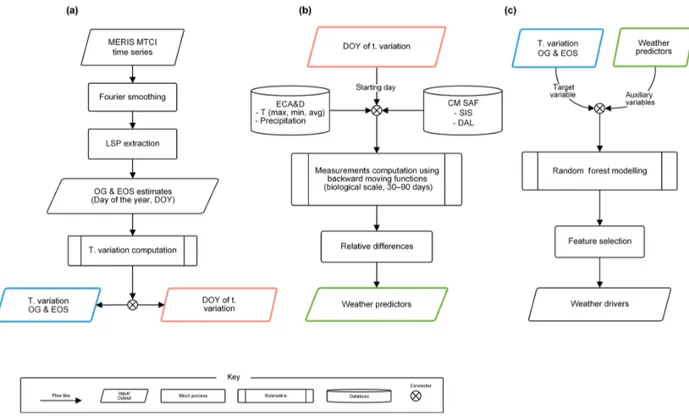
The time series of MERIS MTCI data was used to esti-mate both the onset of greenness (OG) and end of senes-cence (EOS) from 2003 to 2011. Data for every estima-tion year considered 1.5 years of data (from October in the previous year to July in the next year) because the an-nual pattern of vegetation growth in some parts of Europe spans across calendar years, and hence insufficient informa-tion about LSP is captured using a single year of data. The yearly values of OG and EOS were estimated for each im-age pixel of the study area using the methodology described in Dash et al. (2010). This methodology consists of two ma-jor procedures: data smoothing and LSP estimation (Fig. 2a). Smoothed MTCI time-series data were obtained using a dis-crete Fourier transform because of its advantage of requir-ing fewer user-defined parameters compared to other meth-ods (Atkinson et al., 2012). The peak in the annual profile was defined as a point on the phenological curve where the first derivative changes sign from positive to negative. Next, the derived data were searched backward and forward de-parting from the maximum annual peak to estimate the OG and EOS, respectively. OG was defined as a valley at the be-ginning of the growing season point (a change in derivative value from positive to negative), and EOS was defined as a valley point occurring at the decaying end of a phenology cycle (a change in derivative value from negative to posi-tive). These satellite-derived LSP estimates were compared
to ground observations of the thousands of deciduous tree phenology records of the Pan European Phenology network (PEP725) (Rodriguez-Galiano et al., 2015a). This compari-son resulted in a large spatio-temporal correlation of the phe-nology estimates with the spring phenophase (OG vs. leaf unfolding; pseudo-R2=0.70) and autumn phenophase (EOS
vs. autumnal colouring; pseudo-R2=0.71).
Z score values during the study period were used as a
proxy to measure interannual variation in the LSP param-eters. Thez score values for a given year were defined as
the difference from the multi-year mean, normalized by the standard deviation across years. The value of the targeted year was excluded in the computation of multiyear mean to enhance the inter-annual variation (Saleska et al., 2007). The spatio-temporal distribution of spring and autumn LSP
zscore values is shown in Figs. S1 and S2 of the Supplement,
respectively.
To match the spatial resolution of the weather predictors, the LSPzscore values for each year were resampled to a
spatial resolution of 0.25◦×0.25◦ by calculating the me-dian of all the LSPzscore values within this area after
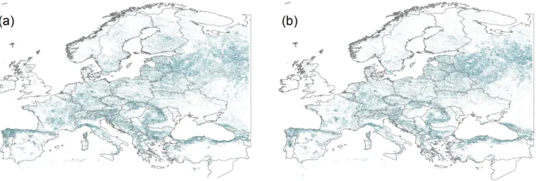
ex-cluding the areas with fewer than 50 LSP estimates and the non-forest pixels according to the Globcover2005 and Glob-cover2009 land cover maps (http://due.esrin.esa.int/page_ globcover.php) (Fig. 1). Only LSP estimates of Globcover forest categories with complete temporal coverage (2003– 2011) were included in the analysis to reduce the likelihood of natural and human disturbances (Potter et al., 2003) and to minimize the effects of human management (i.e. irrigation in croplands). Globcover was selected for its greater consis-tency with the MERIS MTCI time series and its high geolo-cational accuracy (< 150 m) (Bicheron et al., 2011).
2.3 Computation of weather predictors
A suite of weather predictors were computed for each 0.25×0.25◦grid cell associated with the occurrence of
pos-itive or negativez score values in LSP (see Table 1). The
predictors include temporal average values of temperature variables (Tmax,TminandTavg), precipitation, DAL and SIS; temporal cumulated predictors such as growing degree days, chilling, precipitation, SIS and DAL; and the date of specific events such as the onset of greenness (legacy effect for au-tumn phenology modelling), the first freeze or the last freeze, as well as the difference between both dates (freeze period) for the modelling of autumn only. Growing degree days were computed using temperature thresholds of 0 and 5◦. Chilling requirements were computed as the sum of negative temper-atures (tempertemper-atures below 0◦). Freeze was defined as dates with minimum temperatures lower than−2◦(Schwartz et al.,
2006).
The different weather predictors were computed based on the 30 and 90 days previous to the day of the year (DOY) of thez score values in OG and EOS (Fig. 2b) following
3308 V. F. Rodriguez-Galiano et al.: A new approach for modelling changes in phenology
Figure 1.Spatial distribution of Globcover broadleaved deciduous forest and needleleaved evergreen forest in 2005(a)and 2009(b).
Table 1.Predictors used in the modelling of the interannual variation in LSP.
OG anomalies EOS anomalies Averages (M):
Maximum temperature (TX)∗∗ Maximum temperature (TX)∗∗
Minimum temperature (TN)∗∗ Minimum temperature (TN)∗∗
Average temperature (TG)∗∗ Average temperature (TG)∗∗
Precipitation (PP)∗∗ Precipitation (PP)∗∗
Surface incoming shortwave radiation (SIS)∗∗ Surface incoming shortwave radiation (SIS)∗∗
Surface radiation daylight (DAL)∗∗ Surface radiation daylight (DAL)∗∗
Cumulates (C)
Growing degree days (0◦C threshold) (GDD)∗∗ Growing degree days (0◦C threshold) (GDD)∗∗
Growing degree days (5◦C threshold) (GDD)∗∗ Growing degree days (5◦C threshold) (GDD)∗∗
Chilling requirements (CHIL)∗ Chilling requirements (CHIL)∗∗
Precipitation (PP)∗∗ Precipitation (PP)∗∗
Surface incoming shortwave radiation (SIS)∗∗ Surface incoming shortwave radiation (SIS)∗∗
Surface radiation daylight (DAL)∗∗ Surface radiation daylight (DAL)∗∗
Date of specific events
First freeze (FF)∗ First freeze (FF)∗
Last freeze (LF)∗ OGzscore value (OGA) (legacy effect of an advanced or delayed spring)
Period of freeze (PF)∗
∗Predicted over a period of 90 days.∗∗Predicted over a period of the 30 and 90 days previous to the date of thezscore value.
that most phenophases of plant observations in Europe cor-related significantly with weather predictors representing the month of onset and the two preceding months. The chilling requirements for spring modelling and freeze predictors were an exception, as the period for its computation starts 90 days prior to the OG. Relative differences between each predictor and its multi-year average for the same period were com-puted to capture the inter-annual variability in climate vari-ables at the pixel level for every predictor and to facilitate the modelling of climate-driven variation in phenology (Table 1).
2.4 Modelling interannual variation in LSP
com-Figure 2.Flowchart illustrating the methodology.(a)Phenology extraction and interannual variation in LSP computation.(b)Computation
of weather predictors.(c)Modelling of interannual variation in phenology.
pared to global single predictive models, allowing for multi-ple regression models using recursive partitioning (Breiman, 1984). Assembling a single global model might not be rep-resentative of LSP of the entire European continent, when there are many climatic drivers which interact in compli-cated, non-linear ways and may vary spatially and tempo-rally. For the purpose of this paper, an alternative approach is to sub-divide, or partition, the data space into more homoge-neous regions of similar climates and ecological factors.
Regression trees use a sum of squares criterion to split the data into successively more homogeneous subsets contained at many different structural units called nodes. Each of the terminal nodes has attached to it a simple regression which applies in that node only. Therefore, different regressions can be fitted to different data subsets within one single regression tree, which can represent different responses controlled by different drivers (Archibald et al., 2009; Lawler et al., 2006). Additionally, the performance of multiple regression trees can be combined to increase the predictive ability of a single regression tree model, following the RF technique (Fig. 3). The RF method is an innovative machine learning approach that can perform multivariate non-linear regression, combin-ing the performance of numerous regression tree algorithms to predict the interannual variation in OG and EOS. More details regarding the performance and the specific character-istics of a RF model can be seen in Rodriguez-Galiano et al. (2015b, 2014) and Fig. 3.
The RF method was applied to phenological modelling across very large areas and across multiple years simulta-neously: the typical case for satellite-observed LSP. The RF model was fitted to the relation between LSP interannual variation and numerous climate predictor variables computed at biologically relevant rather than human-imposed temporal scales. We restricted our climate data choices to daily data (average, minimum and maximum temperatures, precipita-tion and radiaprecipita-tion) to account for integrative forcing (that is, growing degree days, chilling requirements as well as cu-mulative precipitation and radiation), computed from the ex-act day of the phenological event backwards, rather than us-ing the calendar months. The locations withzscore in LSP
greater than 1 (positive and negative) were selected to build a RF predictive model on OG and EOS. Thezscore values
of OG or EOS for each year were combined together with the different weather predictors. Thezscore values in OG
3310 V. F. Rodriguez-Galiano et al.: A new approach for modelling changes in phenology
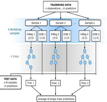
Figure 3. The flowchart of random forest (RF) for regression
(adapted from Rodriguez-Galiano et al., 2015b). The RF method receives a subset of input vectors (n), made up of one phenology
zscore value and the values of the corresponding weather predictors
for a given location and year. RF builds a numberKof regression
trees making them grow from different training data subsets, resam-pling randomly the original data set with replacement. Hence, most data will be used multiple times in different models. On the other hand, when the RF makes a tree grow, it uses the best predictor within a subset of predictors (m) which has been selected randomly
from the overall set of input predictors. These special characteris-tics of RF confer a greater prediction stability and accuracy and, at the same time, avoid the correlation of the different regression tress (RTs), increasing the diversity of patterns that can be learnt from data. The multiple predictions of allKRTs for a given vector used
as training are then averaged to obtain a unique estimation of the phenologyzscore value.
were grown using different subsets of predictors, varying the number of random predictors from 1 to 9. The RF method within the package implemented in the R statistical software was used to build the different models (Liaw and Wiener, 2002).
2.5 Selection of the most important predictors
The RF method can use the out-of-bag subset to estimate the relative importance of each predictor in the model. This prop-erty is especially useful for the present research, as well as for other multivariate biological studies, where it is important to know the physical drivers of the phenomenon under investi-gation (Archibald et al., 2009; Lawler et al., 2006). However, the inclusion of different measures of weather predictors may imply a large increase in the dimensionality of the data sets being used, as these variables are obtained by applying mul-tiple functions or measures to the temperature, precipitation
and radiation time series. On the one hand, more information may be useful for the modelling process; on the other hand, an excessive number of correlated predictors or features can overwhelm the expected increase in accuracy and may intro-duce additional complexity limiting the ability of the method to point to possible cause–effect relationships between in-terannual variation in phenology and their drivers, making interpretation challenging.
A feature selection approach, based on the ability of the RF to assess the relative importance of the predictors, was used to identify the minimum number of drivers which can better explain spring or autumn interannual variation in phe-nology. To assess the importance of each weather predictor, the RF switches one of the input predictors while keeping the rest constant, and it re-evaluates the performance of the model measuring the decrease in node impurity (Breiman, 2001). The differences were averaged over all 2000 trees to compute the general drivers for the interannual variation in Europe. However, different subsets of variables could be used to characterize different climates and ecological factors at every single regression tree model or node (see previous section). In order to reduce the number of drivers the least im-portant predictor was removed iteratively at different steps. Then, a 5-fold cross-validation was applied to obtain a sta-ble estimate of the error of the model built after predictor deletions. Finally, the model with a better trade-off between number of predictors and error was chosen as the basis for interpreting the likely drivers of interannual variation in phe-nology.
3 Results
Numerous models were built on the basis of different pre-dictor combinations considering different temporal windows prior to the spring and autumn phenological events (see sec-tion “Computasec-tion of weather predictors”). The percentage of variation (pseudo-R2)explained by different weather-LSP
models is shown in the supplementary information (Supple-ment Tables S1, S2 and S3). No previous studies have inves-tigated in depth the parametrization of GDD for LSP and cli-mate inter-comparison, unlike for ground phenological stud-ies (Snyder et al., 1999). Although we did not carry out an exhaustive analysis of the optimum GDD parametrization, our results showed a systematic pattern in spring models, pre-senting slightly larger pseudo-R2for models which used 0◦C as a threshold for the computation of GDD (rather than 5◦C). Regarding the length of the temporal windows for weather function computation, spring models using 30 and 90 days for the computation of averaged and cumulative functions were more accurate, whereas for autumn models with 90-day-averaged predictors outperformed the rest.
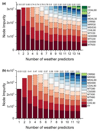
predic-tors”). Spring models were more accurate than autumn, with median relative error values of 10 to 27 % (12 to 1 predic-tor), versus 26 to 60 % of autumn (14 to 1 predictor). Fig-ure 4 shows the pseudo-R2of the models as well as the
rel-ative importance of each predictor. Spring models explained a percentage of the variance up to 81 % (Fig. 4a), whereas autumn explained up to 61 % (Fig. 4b). Cook et al. (2005), using a modelled based on GDD only, explained 63 % on the variance of onset date for mixed and boreal forest. Figure 5 shows the relative error in the prediction of different models after removing the least important predictor. Regarding the relative importance of the drivers, the same ranking in im-portance was observed within the different models of each phenophase, which reflected the stability in the RF impor-tance estimation, and a high reliability of the results (Fig. 4). To interpret the main weather drivers of the interannual vari-ation in phenology, simplified models with reduced num-ber of predictors were selected for spring and autumn (see Sect. 3.5), respectively. The spring model was composed of six predictors (pseudo-R2=0.77 and median relative error
of 10 %) and the autumn model of five predictors
(pseudo-R2=0.59 and median relative error of 28 %) (Fig. 6). Our
re-sults suggest that interannual variation in the onset on green-ness (LSP) of temperate forest species is driven mainly by the daily temperature of the 30 days prior to onset (but not nec-essarily the GDD), with the most important driver being the minimum temperature. Photoperiod was also important; the most accurate empirical prediction was obtained by a com-bined temperature–radiation forcing, integrating the SIS of the previous 90 days. For senescence, temperature was sug-gested to be more important than photoperiod in controlling the senescence process (Archetti et al., 2013; Jeong and Med-vigy, 2014; Vitasse et al., 2009; Yang et al., 2012), with the most important drivers being the date of the first freeze and the accumulation of chilling temperatures. However, we did not observe a legacy effect of a much earlier or later spring onset on the date of senescence. Autumn models that in-cluded the interannual variation (zscore values) in the onset
of greenness did not outperform the remaining models (see Tables S2 and S3) and the relative importance was low in comparison with other drivers.
4 Discussion
The selection and computation of the weather predictors is an important step in phenological modelling. Most of studies on the sensitivity of phenological events to climate used human calendar scales, that is, seasonal or monthly calendar mean or cumulative climate predictors (Maignan et al., 2008a, b; Menzel et al., 2006; Schwartz et al., 2006), overlooking the importance of biological timescales in phenology. However, with the increased availability of daily weather data sets, cur-rent and future studies might benefit from the use of daily in-formation to model the drivers of plants’ circadian timescales
Figure 4.Relative importance of each independent variable in
pre-dicting phenology interannual variation in Europe. Different models derived from the feature selection approach are represented in each column. Numbers given over each column represent the coefficient determination of each model. Plots at the top and bottom represent the spring(a)and autumn(b)interannual variation in LSP,
respec-tively. The names of predictors use the following notation: prefixes M and C represent the mean and cumulated functions; TX, TN and TG: maximum, minimum and average temperature, respectively; PP: precipitation; SIS: surface incoming shortwave radiation; DAL: surface radiation daylight; GDD: growing degree days; CHIL: chill-ing requirements; FF, LF and PF: first, last and period of freeze, respectively.
V . F . Rodriguez-Galiano et al.: A new appr oach for modelling changes in phenology e 5. Relati ve error of the models fitted as a result of the fea-selection approach. Median (interior horizontal line), mean (in-square), 1 and 99 % quantiles (edge of box es), and range (e x-Relati ve errors were calculated for the prediction of 1974 1576 independent observ ations for spring (a) and autumn (b) , vely .See pre vious figure for the weather predictor variables the models, as sho wn on the x axis. date of onset play a more important role (T able s S1, S2 S3). From a computational point of vie w , considering ger temporal windo ws for calculating av erages w ould in-a smoothing ef fect, de grading the information in the whereas cumulati ve functions such as GDD or requirements w ould not be af fected by this ef fect. we ver ,we observ ed a di ver gent response between spring autum n and consi stent throughout the models of each suggests that a biological explanation for this might be plausible. Our study focused on modelling the interannual variation spri ng and autumn LSP and not on predicting the abso-dates of leaf phenology . W e were, thus, modelling rel-ve temporal measurements associated with the same loca-(pix el) to explore the potential ov erall dri vers of changes LSP across Europe. This means adv ances or delays in the when considering the temporal av erage for that partic-pix el ( z score). Understanding the dri vers of interan-variation in LSP amidst background inter -annual vari-is a critical aspect of global change science (de Beurs
Table 2.Correlations between the predictors used in the modelling of spring interannual variation in LSP. Significant correlations between the anomalies and the predictors are given in bold (p< 0.05).
1 2 3 4 5 6 7 8 9 10 11 12 13 14 15 16 17 18 19 20 21 22 23 24 25 26 27
1 Anomaly 1.00 −0.40 −0.43 −0.11 −0.09 −0.12 −0.10 −0.11 −0.10 0.24 −0.03 −0.03 −0.03 −0.14 −0.04 −0.04 −0.33 −0.16 −0.16 −0.04 −0.06 −0.06 −0.45 −0.46 −0.12 −0.31 −0.03
2 GDD090 −0.40 1.00 0.93 0.11 0.14 0.11 0.13 0.11 0.15 −0.64 0.00 −0.01 −0.01 0.23 0.01 0.01 −0.12 −0.06 −0.06 0.04 −0.05 −0.05 0.67 0.64 0.18 −0.11 0.05
3 GDD590 −0.43 0.93 1.00 0.11 0.10 0.11 0.10 0.11 0.11 −0.47 −0.01 −0.01 −0.01 0.16 0.01 0.01 0.03 0.04 0.04 0.06 0.03 0.03 0.74 0.75 0.16 0.03 0.06
4 MTG30 −0.11 0.11 0.11 1.00 0.99 1.00 0.99 1.00 0.98 −0.05 0.89 0.89 0.89 0.20 0.97 0.96 0.02 0.00 0.00 0.31 −0.01 −0.01 0.17 0.15 0.28 0.07 0.31
5 MTG90 −0.09 0.14 0.10 0.99 1.00 0.98 1.00 0.99 1.00 −0.13 0.88 0.88 0.88 0.25 0.96 0.96 −0.03 −0.03 −0.03 0.30 −0.04 −0.04 0.10 0.09 0.29 0.02 0.31
6 MTX30 −0.12 0.11 0.11 1.00 0.98 1.00 0.99 0.99 0.98 −0.04 0.89 0.89 0.88 0.19 0.96 0.96 0.03 0.00 0.00 0.32 −0.01 −0.01 0.18 0.16 0.27 0.08 0.32
7 MTX90 −0.10 0.13 0.10 0.99 1.00 0.99 1.00 0.99 1.00 −0.11 0.89 0.89 0.89 0.23 0.96 0.96 −0.03 −0.03 −0.03 0.30 −0.04 −0.04 0.10 0.09 0.28 0.02 0.31
8 MTN30 −0.11 0.11 0.11 1.00 0.99 0.99 0.99 1.00 0.98 −0.06 0.89 0.89 0.89 0.21 0.96 0.96 0.02 0.01 0.01 0.31 0.00 0.00 0.16 0.14 0.29 0.06 0.31
9 MTN90 −0.10 0.15 0.11 0.98 1.00 0.98 1.00 0.98 1.00 −0.15 0.88 0.88 0.88 0.26 0.96 0.96 −0.04 −0.03 −0.03 0.29 −0.03 −0.03 0.10 0.09 0.30 0.02 0.30
10 CHIL 0.24 −0.64 −0.47 −0.05 −0.13 −0.04 −0.11 −0.06 −0.15 1.00 −0.01 0.00 0.00 −0.25 0.00 0.00 0.28 0.11 0.11 0.03 0.06 0.06 −0.24 −0.26 −0.16 0.26 0.01
11 FF −0.03 0.00 −0.01 0.89 0.88 0.89 0.89 0.89 0.88 −0.01 1.00 1.00 1.00 −0.01 0.88 0.88 −0.04 −0.05 −0.05 0.00 −0.06 −0.06 0.00 −0.01 −0.01 −0.03 0.00
12 LF −0.03 −0.01 −0.01 0.89 0.88 0.89 0.89 0.89 0.88 0.00 1.00 1.00 1.00 −0.01 0.88 0.88 −0.04 −0.05 −0.05 0.00 −0.06 −0.06 −0.01 −0.01 −0.01 −0.03 0.00
13 PF −0.03 −0.01 −0.01 0.89 0.88 0.88 0.89 0.89 0.88 0.00 1.00 1.00 1.00 −0.02 0.88 0.88 −0.04 −0.05 −0.05 0.00 −0.06 −0.06 −0.01 −0.01 −0.01 −0.03 0.00
14 CRR90 −0.14 0.23 0.16 0.20 0.25 0.19 0.23 0.21 0.26 −0.25 −0.01 −0.01 −0.02 1.00 0.20 0.20 0.01 0.06 0.06 0.53 0.04 0.04 0.09 0.07 0.77 0.11 0.58
15 MRR30 −0.04 0.01 0.01 0.97 0.96 0.96 0.96 0.96 0.96 0.00 0.88 0.88 0.88 0.20 1.00 1.00 0.00 −0.03 −0.03 0.31 −0.03 −0.03 0.03 0.03 0.26 0.05 0.31
16 MRR90 −0.04 0.01 0.01 0.96 0.96 0.96 0.96 0.96 0.96 0.00 0.88 0.88 0.88 0.20 1.00 1.00 0.00 −0.03 −0.03 0.31 −0.03 −0.03 0.03 0.02 0.26 0.05 0.31
17 CSIS90 −0.33 −0.12 0.03 0.02 −0.03 0.03 −0.03 0.02 −0.04 0.28 −0.04 −0.04 −0.04 0.01 0.00 0.00 1.00 0.80 0.80 0.16 0.57 0.57 0.22 0.22 0.12 0.96 0.15
18 MSIS30 −0.16 −0.06 0.04 0.00 −0.03 0.00 −0.03 0.01 −0.03 0.11 −0.05 −0.05 −0.05 0.06 −0.03 −0.03 0.80 1.00 1.00 0.06 0.90 0.90 0.23 0.24 0.15 0.77 0.06
19 MSIS90 −0.16 −0.06 0.04 0.00 −0.03 0.00 −0.03 0.01 −0.03 0.11 −0.05 −0.05 −0.05 0.06 −0.03 −0.03 0.80 1.00 1.00 0.06 0.90 0.90 0.23 0.24 0.15 0.77 0.06
20 CDAL90 −0.04 0.04 0.06 0.31 0.30 0.32 0.30 0.31 0.29 0.03 0.00 0.00 0.00 0.53 0.31 0.31 0.16 0.06 0.06 1.00 0.05 0.05 0.11 0.10 0.78 0.28 0.99
21 MDAL30 −0.06 −0.05 0.03 −0.01 −0.04 −0.01 −0.04 0.00 −0.03 0.06 −0.06 −0.06 −0.06 0.04 −0.03 −0.03 0.57 0.90 0.90 0.05 1.00 1.00 0.23 0.23 0.13 0.55 0.05
22 MDAL90 −0.06 −0.05 0.03 −0.01 −0.04 −0.01 −0.04 0.00 −0.03 0.06 −0.06 −0.06 −0.06 0.04 −0.03 −0.03 0.57 0.90 0.90 0.05 1.00 1.00 0.23 0.23 0.13 0.55 0.05
23 GDD030 −0.45 0.67 0.74 0.17 0.10 0.18 0.10 0.16 0.10 −0.24 0.00 −0.01 −0.01 0.09 0.03 0.03 0.22 0.23 0.23 0.11 0.23 0.23 1.00 0.97 0.16 0.23 0.11
24 GDD530 −0.46 0.64 0.75 0.15 0.09 0.16 0.09 0.14 0.09 −0.26 −0.01 −0.01 −0.01 0.07 0.03 0.02 0.22 0.24 0.24 0.10 0.23 0.23 0.97 1.00 0.15 0.24 0.10
25 CRR30 −0.12 0.18 0.16 0.28 0.29 0.27 0.28 0.29 0.30 −0.16 −0.01 −0.01 −0.01 0.77 0.26 0.26 0.12 0.15 0.15 0.78 0.13 0.13 0.16 0.15 1.00 0.18 0.79
26 CSIS30 −0.31 −0.11 0.03 0.07 0.02 0.08 0.02 0.06 0.02 0.26 −0.03 −0.03 −0.03 0.11 0.05 0.05 0.96 0.77 0.77 0.28 0.55 0.55 0.23 0.24 0.18 1.00 0.28
27 CDAL30 −0.03 0.05 0.06 0.31 0.31 0.32 0.31 0.31 0.30 0.01 0.00 0.00 0.00 0.58 0.31 0.31 0.15 0.06 0.06 0.99 0.05 0.05 0.11 0.10 0.79 0.28 1.00
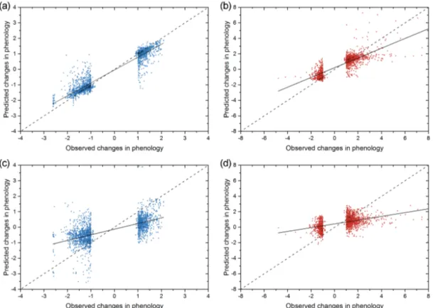
Figure 6.Scatterplots between observed anomalies in LSP and the predictions calculated using a selection of weather predictors (see Figs. 2
and 3). Plots for spring phenology are shown on the left panel (blue;a, c) and autumn on the right (red;b, d). Random-forest (RF) predictions
are given in the upper panel(a, b)and those of the linear regression in the bottom(c, d)panel. The dashed lines represent an exact 1 : 1
relationship (expected fitting); the solid lines show a linear regression of these data. The explained variances (percentageR2)and RMSE
values are 90 % and 0.43 (spring RF model), 68 % and 0.92 (autumn RF model), 39 % and 1.04 (spring linear model), and 25 % 1.40 (autumn linear model).
and Henebry, 2005; Zhao et al., 2013). To this end, the RF method is particularly pertinent, as it allows the assess-ment of the importance of the predictors (Fig. 4). Our find-ings reveal that the accuracy of growing degree-day-based models might be overestimated using linear regression mod-els and that non-linear multivariate relationships between temperature (especially minimum temperature) and radia-tion are needed to describe the relaradia-tions between phenology and weather drivers. This supports the findings of Stöckli et al. (2011), who explained temperate phenology using a com-bination of light and temperature. The highlighted impor-tance of minimum temperatures might be related to the fact that minimum temperature is a better indicator of weather changes than either the average or maximum temperature (Duncan et al., 2014; Jolly et al., 2005). Regarding GDD, although it has been applied extensively to predict vegetation phenophases, it is currently debated whether such models can detect when multiple environmental drivers are required to initiate a phenological event, or detect drivers that are rela-tively static across time, such as photoperiods (Stöckli et al., 2011). Our results reveal that multiple environmental drivers are required to initiate phenological events of Europe and
also showed that the role of GDD alone in driving spring phe-nology might be overestimated due to an over-reliance on lin-ear models. GDD had the largest linlin-ear association with veg-etation phenology interannual variation, while the linear cor-relation between LSP and others drivers that were revealed as very important by the RF was small (see Tables 2 and 3). A simple linear analysis between GDD and phenology could ignore complex non-linear associations between phe-nology and predictors as well as synergies between weather drivers. Regarding the senescence phase, the autumn models had a weaker predictive power compared to the spring mod-els. There is still a lack of clear understanding of mechanism autumn senescence; however, temperature, and particularly the dates of freeze, has been suggested as a major driver of autumn phenology.
V . F . Rodriguez-Galiano et al.: A new appr oach for modelling changes in phenology
Table 3.Correlations between the predictors used in the modelling of autumn interannual variation in LSP. Significant correlations between the anomalies and the predictors are given in bold (p< 0.05).
1 2 3 4 5 6 7 8 9 10 11 12 13 14 15 16 17 18 19 20 21 22 23 24 25 26 27
1 Anomaly 1 0.10 0.31 0.34 0.33 0.36 0.28 0.30 0.28 0.27 0.26 0.34 0.01 −0.03 0.34 0.07 0.07 0.04 −0.05 −0.05 −0.05 0.00 −0.01 −0.08 −0.08 −0.09 −0.15
2 OGA 0.10 1.00 0.06 0.08 0.14 0.16 0.05 0.15 0.02 0.07 0.05 0.19 −0.02 −0.04 0.01 0.02 −0.05 −0.07 0.06 −0.02 −0.02 −0.10 −0.11 0.01 0.01 −0.06 −0.10
3 GDD030 0.31 0.06 1.00 0.97 0.54 0.58 0.94 0.53 0.88 0.42 0.87 0.62 −0.54 −0.52 0.25 0.09 0.10 0.11 0.03 −0.09 −0.09 −0.01 0.01 −0.22 −0.22 −0.11 −0.22
4 GDD530 0.34 0.08 0.97 1.00 0.53 0.60 0.86 0.49 0.80 0.37 0.80 0.59 −0.41 −0.40 0.24 0.11 0.11 0.10 0.07 −0.10 −0.10 −0.03 −0.01 −0.23 −0.23 −0.15 −0.25
5 GDD090 0.33 0.14 0.54 0.53 1.00 0.98 0.49 0.95 0.54 0.90 0.36 0.85 −0.14 −0.24 0.12 0.05 0.13 0.09 −0.15 −0.07 −0.07 0.04 −0.05 −0.14 −0.14 0.08 −0.14
6 GDD590 0.36 0.16 0.58 0.60 0.98 1.00 0.49 0.92 0.54 0.85 0.37 0.84 −0.10 −0.20 0.14 0.07 0.13 0.09 −0.11 −0.07 −0.07 0.02 −0.06 −0.14 −0.14 0.04 −0.19
7 MTG30 0.28 0.05 0.94 0.86 0.49 0.49 1.00 0.56 0.93 0.44 0.94 0.63 −0.71 −0.66 0.24 0.04 0.10 0.09 −0.01 −0.02 −0.02 0.02 0.05 −0.13 −0.13 −0.09 −0.17
8 MTG90 0.30 0.15 0.53 0.49 0.95 0.92 0.56 1.00 0.61 0.93 0.43 0.89 −0.28 −0.36 0.12 −0.01 0.13 0.09 −0.18 0.02 0.02 0.07 −0.01 −0.03 −0.03 0.09 −0.11
9 MTX30 0.28 0.02 0.88 0.80 0.54 0.54 0.93 0.61 1.00 0.58 0.78 0.60 −0.58 −0.54 0.20 −0.09 0.12 0.07 −0.09 0.03 0.03 0.23 0.14 −0.09 −0.09 0.17 −0.06
10 MTX90 0.27 0.07 0.42 0.37 0.90 0.85 0.44 0.93 0.58 1.00 0.28 0.73 −0.16 −0.24 0.09 −0.05 0.13 0.05 −0.31 0.02 0.02 0.17 0.07 −0.03 −0.03 0.23 0.07
11 MTN30 0.26 0.05 0.87 0.80 0.36 0.37 0.94 0.43 0.78 0.28 1.00 0.61 −0.76 −0.70 0.26 0.16 0.08 0.09 0.08 −0.06 −0.06 −0.17 −0.04 −0.14 −0.14 −0.30 −0.24
12 MTN90 0.34 0.19 0.62 0.59 0.85 0.84 0.63 0.89 0.60 0.73 0.61 1.00 −0.39 −0.48 0.19 0.12 0.13 0.12 0.04 −0.02 −0.02 −0.07 −0.12 −0.06 −0.06 −0.08 −0.31
13 CHIL30 0.01 −0.02 −0.54 −0.41 −0.14 −0.10 −0.71 −0.28 −0.58 −0.16 −0.76 −0.39 1.00 0.91 −0.08 −0.05 0.00 0.01 −0.05 −0.05 −0.05 0.09 −0.01 −0.01 −0.01 0.17 0.10
14 CHIL90 −0.03 −0.04 −0.52 −0.40 −0.24 −0.20 −0.66 −0.36 −0.54 −0.24 −0.70 −0.48 0.91 1.00 −0.09 −0.04 0.00 0.01 −0.05 −0.08 −0.08 0.08 0.01 −0.04 −0.04 0.16 0.15
15 FF 0.34 0.01 0.25 0.24 0.12 0.14 0.24 0.12 0.20 0.09 0.26 0.19 −0.08 −0.09 1.00 −0.10 0.05 0.04 −0.08 0.01 0.01 0.01 0.07 −0.05 −0.05 −0.08 −0.04
16 CRR30 0.07 0.02 0.09 0.11 0.05 0.07 0.04 −0.01 −0.09 −0.05 0.16 0.12 −0.05 −0.04 −0.10 1.00 0.12 0.04 0.51 −0.17 −0.17 −0.42 −0.25 −0.12 −0.12 −0.46 −0.25
17 MRR30 0.07 −0.05 0.10 0.11 0.13 0.13 0.10 0.13 0.12 0.13 0.08 0.13 0.00 0.00 0.05 0.12 1.00 0.47 0.08 −0.03 −0.03 −0.02 −0.03 −0.03 −0.03 −0.02 −0.04
18 MRR90 0.04 −0.07 0.11 0.10 0.09 0.09 0.09 0.09 0.07 0.05 0.09 0.12 0.01 0.01 0.04 0.04 0.47 1.00 0.06 −0.01 −0.01 −0.02 −0.04 −0.02 −0.02 −0.02 −0.08
19 CRR90 −0.05 0.06 0.03 0.07 −0.15 −0.11 −0.01 −0.18 −0.09 −0.31 0.08 0.04 −0.05 −0.05 −0.08 0.51 0.08 0.06 1.00 −0.04 −0.05 −0.14 −0.18 −0.05 −0.05 −0.20 −0.39
20 MSIS30 −0.05 −0.02 −0.09 −0.10 −0.07 −0.07 −0.02 0.02 0.03 0.02 −0.06 −0.02 −0.05 −0.08 0.01 −0.17 −0.03 −0.01 −0.04 1.00 1.00 0.56 0.66 0.88 0.88 0.05 −0.04
21 MSIS90 −0.05 −0.02 −0.09 −0.10 −0.07 −0.07 −0.02 0.02 0.03 0.02 −0.06 −0.02 −0.05 −0.08 0.01 −0.17 −0.03 −0.01 −0.05 1.00 1.00 0.55 0.66 0.88 0.88 0.05 −0.04
22 CSIS30 0.00 −0.10 −0.01 −0.03 0.04 0.02 0.02 0.07 0.23 0.17 −0.17 −0.07 0.09 0.08 0.01 −0.42 −0.02 −0.02 −0.14 0.56 0.55 1.00 0.80 0.30 0.30 0.66 0.28
23 CSIS90 −0.01 −0.11 0.01 −0.01 −0.05 −0.06 0.05 −0.01 0.14 0.07 −0.04 −0.12 −0.01 0.01 0.07 −0.25 −0.03 −0.04 −0.18 0.66 0.66 0.80 1.00 0.31 0.31 0.18 0.40
24 MDAL30 −0.08 0.01 −0.22 −0.23 −0.14 −0.14 −0.13 −0.03 −0.09 −0.03 −0.14 −0.06 −0.01 −0.04 −0.05 −0.12 −0.03 −0.02 −0.05 0.88 0.88 0.30 0.31 1.00 1.00 0.05 −0.05
25 MDAL90 −0.08 0.01 −0.22 −0.23 −0.14 −0.14 −0.13 −0.03 −0.09 −0.03 −0.14 −0.06 −0.01 −0.04 −0.05 −0.12 −0.03 −0.02 −0.05 0.88 0.88 0.30 0.31 1.00 1.00 0.05 −0.05
26 CDAL30 −0.09 −0.06 −0.11 −0.15 0.08 0.04 −0.09 0.09 0.17 0.23 −0.30 −0.08 0.17 0.16 −0.08 −0.46 −0.02 −0.02 −0.20 0.05 0.05 0.66 0.18 0.05 0.05 1.00 0.41
Data availability
The dataset used in the modelling can be accessed at: https: //zenodo.org/record/54016.
The Supplement related to this article is available online at doi:10.5194/bg-13-3305-2016-supplement.
Author contributions. Victor F. Rodriguez-Galiano,
Jadunan-dan Dash, Peter M. Atkinson and J. Ojeda-Zujar conceived and designed the experiments; Victor F. Rodriguez-Galiano performed the experiments; Victor F. Rodriguez-Galiano, Manuel Sanchez-Castillo and Jadunandan Dash contributed analysis tools; Vic-tor F. Rodriguez-Galiano drafted the paper. All authors contributed to the final paper.
Acknowledgements. The first author is a Marie Curie Grant holder
(reference FP7-PEOPLE-2012-IEF-331667). The authors are grate-ful for the financial support given by the European Commission un-der the Seventh Framework Programme and the Spanish MINECO (project BIA2013-43462-P). Peter M. Atkinson is grateful to the University of Utrecht for supporting him with The Belle van Zuylen Chair. We acknowledge the E-OBS data set from the EU-FP6 project ENSEMBLES (http://ensembles-eu.metoffice.com) and the data providers in the ECA&D project (http://www.ecad.eu). Surface radiation data were obtained from EUMETSAT’s Satellite Application Facility on Climate Monitoring (CM SAF).
Edited by: A. Ibrom
References
Archetti, M., Richardson, A. D., O’Keefe, J., and Delpierre, N.: Pre-dicting Climate Change Impacts on the Amount and Duration of Autumn Colors in a New England Forest, PLoS ONE, 8, e57373, doi:10.1371/journal.pone.0057373, 2013.
Archibald, S., Roy, D. P., van Wilgen, B. W., and Scholes, R. J.: What limits fire? An examination of drivers of burnt area in Southern Africa, Glob. Change Biol., 15, 613–630, 2009. Atkinson, P. M., Jeganathan, C., Dash, J., and Atzberger, C.:
Inter-comparison of four models for smoothing satellite sensor time-series data to estimate vegetation phenology, Remote Sens. Env-iron., 123, 400–417, 2012.
Barriopedro, D., Fischer, E. M., Luterbacher, J., Trigo, R. M., and García-Herrera, R.: The Hot Summer of 2010: Redrawing the Temperature Record Map of Europe, Science, 332, 220–224, 2011.
Bicheron, P., Amberg, V., Bourg, L., Petit, D., Huc, M., Miras, B., Brockmann, C., Hagolle, O., Delwart, S., Ranera, F., Leroy, M., and Arino, O.: Geolocation Assessment of MERIS GlobCover Orthorectified Products, IEEE T. Geosci. Remote, 49, 2972– 2982, 2011.
Breiman, L.: Classification and regression trees, Chapman & Hall/CRC, Monterey, CA, 1984.
Breiman, L.: Random forests, Mach. Learning, 45, 5–32, 2001. Brown, M. E. and de Beurs, K. M.: Evaluation of multi-sensor
semi-arid crop season parameters based on NDVI and rainfall, Remote Sens. Environ., 112, 2261–2271, 2008.
Cook, B. I., Smith, T. M., and Mann, M. E.: The North Atlantic Os-cillation and regional phenology prediction over Europe, Glob. Change Biol., 11, 919–926, 2005.
Darling, E. S., Alvarez-Filip, L., Oliver, T. A., McClanahan, T. R., and Côté, I. M.: Evaluating life-history strategies of reef corals from species traits, Ecol. Lett., 15, 1378–1386, 2012.
Dash, J., Jeganathan, C., and Atkinson, P. M.: The use of MERIS Terrestrial Chlorophyll Index to study spatio-temporal variation in vegetation phenology over India, Remote Sens. Environ., 114, 1388–1402, 2010.
de Beurs, K. M. and Henebry, G. M.: Land surface phenology and temperature variation in the International Geosphere-Biosphere Program high-latitude transects, Glob. Change Biol., 11, 779– 790, 2005.
De Beurs, K. M. and Henebry, G. M.: Northern annular mode ef-fects on the land surface phenologies of northern Eurasia, J. Cli-mate, 21, 4257–4279, 2008.
Delbart, N., Picard, G., Le Toan, T., Kergoat, L., Quegan, S., Wood-ward, I., Dye, D., and Fedotova, V.: Spring phenology in boreal Eurasia over a nearly century time scale, Glob. Change Biol., 14, 603–614, 2008.
Duncan, J. M. A., Dash, J., and Atkinson, P. M.: Elucidating the impact of temperature variability and extremes on cereal crop-lands through remote sensing, Glob. Change Biol., 21, 1541– 1551, 2014.
Fu, Y. S. H., Campioli, M., Vitasse, Y., De Boeck, H. J., Van Den Berge, J., AbdElgawad, H., Asard, H., Piao, S., Deckmyn, G., and Janssens, I. A.: Variation in leaf flushing date influences au-tumnal senescence and next year’s flushing date in two temperate tree species, P. Natl. Acad. Sci. USA, 111, 7355–7360, 2014. Haylock, M. R., Hofstra, N., Klein Tank, A. M. G., Klok,
E. J., Jones, P. D., and New, M.: A European daily high-resolution gridded data set of surface temperature and pre-cipitation for 1950–2006, J. Geophys. Res., 113, D20119, doi:10.1029/2008JD010201, 2008.
Ivits, E., Cherlet, M., Tóth, G., Sommer, S., Mehl, W., Vogt, J., and Micale, F.: Combining satellite derived phenology with cli-mate data for clicli-mate change impact assessment, Global Planet. Change, 88–89, 85–97, 2012.
Jeganathan, C., Dash, J., and Atkinson, P. M.: Remotely sensed trends in the phenology of northern high latitude terrestrial veg-etation, controlling for land cover change and vegetation type, Remote Sens. Environ., 143, 154–170, 2014.
Jeong, S.-J. and Medvigy, D.: Macroscale prediction of autumn leaf coloration throughout the continental United States, Global Ecol. Biogeogr., 23, 1245–1254, 2014.
Jeong, S.-J., Ho, C.-H., Gim, H.-J., and Brown, M. E.: Phenology shifts at start vs. end of growing season in temperate vegetation over the Northern Hemisphere for the period 1982–2008, Glob. Change Biol., 17, 2385–2399, 2011.
3316 V. F. Rodriguez-Galiano et al.: A new approach for modelling changes in phenology
Karlsen, S. R., Solheim, I., Beck, P. S. A., Hogda, K. A., Wielgo-laski, F. E., and Tommervik, H.: Variability of the start of the growing season in Fennoscandia, 1982–2002, Int. J. Biometeo-rol., 51, 513–524, 2007.
Lawler, J. J., White, D., Neilson, R. P., and Blaustein, A. R.: Predict-ing climate-induced range shifts: Model differences and model reliability, Glob. Change Biol., 12, 1568–1584, 2006.
Lebourgeois, F., Pierrat, J. C., Perez, V., Piedallu, C., Cecchini, S., and Ulrich, E.: Simulating phenological shifts in French temper-ate forests under two climatic change scenarios and four driv-ing global circulation models, Int. J. Biometeorol., 54, 563–581, 2010.
Liaw, A. and Wiener, M.: Classification and Regression by random-Forest, R News, 2/3, 18–22, 2002.
Luterbacher, J., Dietrich, D., Xoplaki, E., Grosjean, M., and Wan-ner, H.: European Seasonal and Annual Temperature Variabil-ity, Trends, and Extremes Since 1500, Science, 303, 1499–1503, 2004.
Maignan, F., Bréon, F. M., Bacour, C., Demarty, J., and Poirson, A.: Interannual vegetation phenology estimates from global AVHRR measurements: Comparison with in situ data and applications, Remote Sens. Environ., 112, 496–505, 2008a.
Maignan, F., Bréon, F. M., Vermote, E., Ciais, P., and Viovy, N.: Mild winter and spring 2007 over western Europe led to a widespread early vegetation onset, Geophys. Res. Lett., 35, L02404, doi:10.1029/2007GL032472, 2008b.
Menzel, A.: Phenology: Its Importance to the Global Change Com-munity, Climatic Change, 54, 379–385, 2002.
Menzel, A., Sparks, T. H., Estrella, N., and Eckhardt, S.: ’SSW to NNE’ – North Atlantic Oscillation affects the progress of seasons across Europe, Glob. Change Biol., 11, 909–918, 2005. Menzel, A., Sparks, T. H., Estrella, N., Koch, E., Aaasa, A., Ahas,
R., Alm-Kübler, K., Bissolli, P., Braslavská, O., Briede, A., Chmielewski, F. M., Crepinsek, Z., Curnel, Y., Dahl, Å., Defila, C., Donnelly, A., Filella, Y., Jatczak, K., Måge, F., Mestre, A., Nordli, Ø., Peñuelas, J., Pirinen, P., Remišová, V., Scheifinger, H., Striz, M., Susnik, A., Van Vliet, A. J. H., Wielgolaski, F. E., Zach, S., and Zust, A.: European phenological response to cli-mate change matches the warming pattern, Glob. Change Biol., 12, 1969–1976, 2006.
Morisette, J. T., Richardson, A. D., Knapp, A. K., Fisher, J. I., Graham, E. A., Abatzoglou, J., Wilson, B. E., Breshears, D. D., Henebry, G. M., Hanes, J. M., and Liang, L.: Tracking the rhythm of the seasons in the face of global change: phenological research in the 21st century, Front. Ecol. Environ., 7, 253–260, 2008. Müller, R. and Trentmann, J.: CM SAF Meteosat Surface
Radiation Daylight Data Set 1.0 – Monthly Means/Daily Means, Satellite Application Facility on Climate Monitor-ing, doi:10.5676/EUM_SAF_CM/DAL_MVIRI_SEVIRI/V001, 2013.
Myneni, R. B., Keeling, C. D., Tucker, C. J., Asrar, G., and Nemani, R. R.: Increased plant growth in the northern high latitudes from 1981 to 1991, Nature, 386, 698–702, 1997.
Pau, S., Wolkovich, E. M., Cook, B. I., Davies, T. J., Kraft, N. J. B., Bolmgren, K., Betancourt, J. L., and Cleland, E. E.: Predicting phenology by integrating ecology, evolution and climate science, Glob. Change Biol., 17, 3633–3643, 2011.
Peñuelas, J.: Phenology feedbacks on climate change, Science, 324, 887-888, 2009.
Peñuelas, J. and Filella, I.: Phenology: Responses to a warming world, Science, 294, 793–795, 2001.
Posselt, R., Müller, R., Stöckli, R., and Trentmann, J.: CM SAF Surface Radiation MVIRI Data Set 1.0 – Monthly Means/Daily Means/Hourly Means, Satellite Application Facility on Climate Monitoring, doi:10.5676/EUM_SAF_CM/RAD_MVIRI/V001, 2011.
Posselt, R., Mueller, R. W., Stöckli, R., and Trentmann, J.: Re-mote sensing of solar surface radiation for climate monitoring – the CM-SAF retrieval in international comparison, Remote Sens. Environ., 118, 186–198, 2012.
Post, E. and Stenseth, N. C.: Climatic variability, plant phenology, and northern ungulates, Ecology, 80, 1322–1339, 1999. Potter, C., Tan, P. N., Steinbach, M., Klooster, S., Kumar, V.,
My-neni, R., and Genovese, V.: Major disturbance events in terres-trial ecosystems detected using global satellite data sets, Glob. Change Biol., 9, 1005–1021, 2003.
Rafferty, N. E., CaraDonna, P. J., Burkle, L. A., Iler, A. M., and Bronstein, J. L.: Phenological overlap of interacting species in a changing climate: an assessment of available approaches, Ecol. Evol., 3, 3183–3193, 2013.
Rodriguez-Galiano, V. F., Chica-Olmo, M., and Chica-Rivas, M.: Predictive modelling of gold potential with the integration of multisource information based on random forest: a case study on the Rodalquilar area, Southern Spain, Int. J. Geogr. Inf. Sci., 28, 1336–1354, 2014.
Rodriguez-Galiano, V., Dash, J., and Atkinson, P. M.: Inter-comparison of satellite sensor land surface phenology and ground phenology in Europe, Geophys. Res. Lett., 42, 2253– 2260, 2015a.
Rodriguez-Galiano, V., Sanchez-Castillo, M., Chica-Olmo, M., and Chica-Rivas, M.: Machine learning predictive models for mineral prospectivity: An evaluation of neural networks, random forest, regression trees and support vector machines, Ore Geol. Rev., 71, 804–818, 2015b.
Rutishauser, T., Luterbacher, J., Defila, C., Frank, D., and Wan-ner, H.: Swiss spring plant phenology 2007: Extremes, a multi-century perspective, and changes in temperature sensitivity, Geo-phys. Res. Lett., 35, L05703, doi:10.1029/2007GL032545, 2008. Saleska, S. R., Didan, K., Huete, A. R., and Da Rocha, H. R.: Ama-zon forests green-up during 2005 drought, Science, 318, 612 pp., doi:10.1126/science.1146663, 2007.
Schwartz, M. D., Ahas, R., and Aasa, A.: Onset of spring starting earlier across the Northern Hemisphere, Glob. Change Biol., 12, 343–351, 2006.
Snyder, R. L., Spano, D., Cesaraccio, C., and Duce, P.: Determining degree-day thresholds from field observations, Int. J. Biometeo-rol., 42, 177–182, 1999.
Stöckli, R., Rutishauser, T., Dragoni, D., O’Keefe, J., Thornton, P. E., Jolly, M., Lu, L., and Denning, A. S.: Remote sensing data assimilation for a prognostic phenology model, J. Geophys. Res.-Biogeo., 113, G04021, doi:10.1029/2008JG000781, 2008. Stöckli, R., Rutishauser, T., Baker, I., Liniger, M. A., and Denning,
A. S.: A global reanalysis of vegetation phenology, J. Geophys. Res.-Biogeosci., 116, G03020, doi:10.1029/2010JG001545, 2011.
Vitasse, Y., Delzon, S., Dufrêne, E., Pontailler, J. Y., Louvet, J. M., Kremer, A., and Michalet, R.: Leaf phenology sensitivity to tem-perature in European trees: Do within-species populations ex-hibit similar responses?, Agr. Forest Meteorol., 149, 735–744, 2009.
Yang, X., Mustard, J. F., Tang, J. W., and Xu, H.: Regional-scale phenology modeling based on meteorological records and remote sensing observations, J. Geophys. Res.-Biogeo., 117, G03029, doi:10.1029/2012jg001977, 2012.
Yu, R., Schwartz, M. D., Donnelly, A., and Liang, L.: An observation-based progression modeling approach to spring and autumn deciduous tree phenology, Int. J. Biometeorol., 60, 335– 349, doi:10.1007/s00484-015-1031-9 2016.
Zhang, X., Friedl, M. A., Schaaf, C. B., and Strahler, A. H.: Climate controls on vegetation phenological patterns in northern mid- and high latitudes inferred from MODIS data, Glob. Change Biol., 10, 1133–1145, 2004.
Zhao, M. F., Peng, C. H., Xiang, W. H., Deng, X. W., Tian, D. L., Zhou, X. L., Yu, G. R., He, H. L., and Zhao, Z. H.: Plant phe-nological modeling and its application in global climate change research: overview and future challenges, Environ. Rev., 21, 1– 14, 2013.