www.adv-radio-sci.net/9/335/2011/ doi:10.5194/ars-9-335-2011
© Author(s) 2011. CC Attribution 3.0 License.
Radio Science
Meteor radar measurements of mean winds and tides over Collm
(51.3
◦
N, 13
◦
E) and comparison with LF drift measurements
2005–2007
C. Jacobi
Institute for Meteorology, University of Leipzig, Stephanstr. 3, 04103 Leipzig, Germany
Abstract. An all-sky VHF meteor radar (MR) has been continuously operated at Collm (51.3◦N, 13◦E) since sum-mer 2004. The radar measures meteor parameters, diffusion coefficients, and horizontal winds in the mesopause region. There exists a temporal overlap of the MR wind measure-ments with co-located low-frequency (LF) ionospheric drift measurements until 2007. Comparison of MR and LF semid-iurnal tidal phases allows to empirically determine the vir-tual height overestimation of LF reflection heights due to the group retardation of LF waves. LF reference heights have to be reduced by up to 20 km to match real heights. Correc-tion of LF heights for group retardaCorrec-tion allows to determine the wind underestimation by the LF method compared with meteor radar measurements and opens the possibility to con-tinue long-term trend analysis using mesosphere/lower ther-mosphere winds.
1 Introduction
As background information for linear models, for valida-tion purposes, and for estimavalida-tion of further derived param-eters there is a need for empirical models of wind paramparam-eters such as prevailing winds and tidal parameters in the meso-sphere/lower thermosphere (MLT) region. The MLT is of special interest because its structure is mainly dynamically driven and represents to a certain degree the boundary be-tween middle and upper atmosphere. To accomplish global empirical models, there is a need to construct and updates models, e.g., from radar measurements at single sites.
Operational radars used for MLT wind measurements in general either use the Doppler shift of the reflected radio wave, or apply the spaced receiver (D1) method. While the
Correspondence to:C. Jacobi ([email protected])
former is the usual method for meteor radars (MR), the lat-ter has been used for the conventional analysis of medium frequency (MF) radars as well as for the low-frequency (LF) method applied, e.g., with earlier measurements over Collm, Germany. MR and D1 wind comparisons have provided hints to systematic differences between the results of the two meth-ods (Hocking and Thayaparan, 1997; Manson et al., 2004; Hall et al., 2005). Jacobi et al. (2009) compared LF, MR and MF winds of one year, and found that MF and LF winds are smaller than MR ones and the differences increase with height. Literature results in all cases indicate that generally winds measured using MF and LF are smaller than those from MR, while the reasons and details of these differences are still under discussion.
336 C. Jacobi: Meteor radar measurements of mean winds and tides over Collm 2 Measurements
2.1 Collm meteor radar
A VHF all-sky MR is operated at Collm (51.3◦N, 13◦E) on 36.2 MHz since summer 2004. Pulse repetition frequency is 2144 Hz, but is effectively reduced to 536 Hz, due to 4-point coherent integration. Power is 6 kW and a 3-element Yagi is used as transmitting antenna. The sampling resolution is 1.87 ms. The pulse width is 13 µs and the receiver bandwidth is 50 kHz. The angular and range resolutions are∼2◦ and 2 km, respectively. The wind measurement principle is the detection of the Doppler shift of the reflected radio waves from ionised meteor trails, which delivers radial wind veloc-ity along the line of sight of the radio wave. An interferom-eter, consisting of five 2-element Yagi antennas arranged as an asymmetric cross is used to detect azimuth and elevation angle from phase comparisons of individual receiver antenna pairs. Together with range measurements this enables the meteor trail position detection. The raw data collected con-sist of azimuth and elevation angle, wind velocity along the line of sight, and meteor height. The data collection proce-dure is also described in detail by Hocking et al. (2001).
The individual meteor trail reflection heights roughly vary between 75 and 110 km, with a maximum around 90 km (Stober et al., 2008). In standard configuration, the data are binned in 6 different not overlapping height gates centred at 82, 85, 88, 91, 94, and 98 km. Individual radial winds cal-culated from the meteors are collected to form half-hourly mean values using a least squares fit of the horizontal wind components to the raw data under the assumption that verti-cal winds are small (Hocking et al., 2001). An outlier rejec-tion is added.
2.2 Collm LF lower ionospheric drifts
At Collm, MLT winds have also been obtained by D1 LF radio wind measurements from 1959-2008, using the iono-spherically reflected sky wave of three commercial radio transmitters. The data were combined to half-hourly zonal and meridional mean wind values. The virtual reflection heights, varying between about 80 and 120 km, have been estimated between late 1982 and 2007 using measured travel time differences between the separately received ionospheri-cally reflected sky wave and the ground wave (K¨urschner et al., 1987). These heights may drastically overestimate the real heights owing to group retardation of the LF radio wave. The LF reference heights vary systematically in the course of one day (e.g. K¨urschner et al., 1987). In addition, due to increased absorption during daylight hours, regular daily data gaps are present, which are particularly long in sum-mer. Therefore, obtaining the means through simple aver-aging of data of one height gate is not possible, and a spe-cial regression analysis based on Groves (1959) is necessary (K¨urschner and Schminder, 1986).
2.3 Prevailing wind and tidal analysis
For the estimation of LF monthly mean wind parameters, a multiple regression analysis with quadratically height-dependent coefficients is used to determine the monthly mean prevailing wind and the semidiurnal tidal wind from the half-hourly wind components (K¨urschner and Schmin-der, 1986; Jacobi et al., 1999; K¨urschner and Jacobi, 2005), i.e. modeling the winds at timet as:
vz(t )= p X
k=0
n
hkak,z+bk,zhksinωt+ck,zhkcosωt o
+ε, (1)
vm(t )= p X
k=0
n
hkak,m+bk,mhksinωt+ck,mhkcosωt o
+ε, (2) with p=2 for a quadratic height dependence, vz(t ) and vm(t ) as the zonal and meridional measured half-hourly winds,has the (virtual) height andω=2π/12 h as the fre-quency of the SDT. Then, the zonal (v0z) and meridional (v0m)mean winds are estimated as
v0z(h)= p X
k=0
ak,zhk, v0m(h)= p X
k=0
ak,mhk, (3) and the estimates of the amplitudesv2zand zonal phasesT2z of the SDT are:
v2z(h)= v u u t p X k=0 bk,zhk
!2 +
p X
k=0 ck,zhk
!2
, (4)
T2z(h)= 1 ωatan p P k=0 bk,zhk
p P
k=0 ck,zhk
. (5)
Meridional amplitudesv2mand phasesT2mare calculated ac-cordingly. In order to improve the separation and the spec-tral selectivity of the evaluation of the tidal components in the presence of data gaps, circular polarization of the SDT horizontal components is assumed, thus
bk,m= −ck,z, and ck,m=bk,z, (6) (K¨urschner, 1991), which of course results inv2m=v2zand T2m=T2z-3 h. This assumption is justified at higher midlat-itudes (Jacobi et at., 1999).
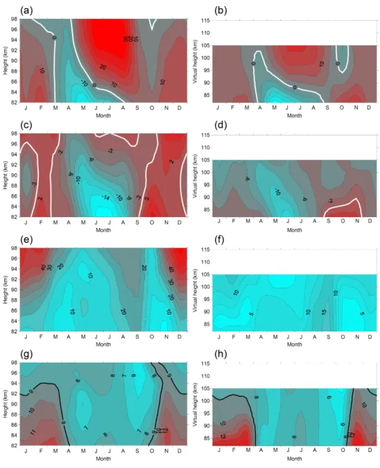
Fig. 1.MLT wind parameters as measured with MR (left) and LF (right). Parameters are zonal prevailing wind(a),(b), meridional prevailing wind(c),(d), SDT amplitude(e),(f), and zonal SDT phase(g),(h). Values are given in m/s, except for the phases given in LT. Height-time cross-sections are based on monthly mean winds and tidal parameters.
3 2004–2007 mean winds measured by meteor radar and LF
3-year mean monthly mean prevailing winds, SDT ampli-tudes and zonal phases are shown in Fig. 1. MR winds are presented on the left, LF winds on the right hand side. Note that the height scaling of the LF winds differs from the MR one in order to achieve approximate correspondence of the wind systems. The gross features of both prevailing wind and SDT seasonal cycle are similar with both mea-surements, although some details differ as, e.g., southerly meridional winds in winter (except for January) measured
338 C. Jacobi: Meteor radar measurements of mean winds and tides over Collm
Fig. 2. Example of SDT vertical phase profiles observed by MR and LF. The blue arrows demonstrate the method of real height es-timation.
The most striking feature is the strong underestimation of LF tidal amplitudes and, less strongly expressed, zonal pre-vailing winds in summer. This is clearly an effect of the spaced receiver bias. To quantify this effect, however, a height correction has to be applied first. This correction is not possible on a physical basis, since the actual D region electron density profile is not known. Therefore an empirical statistical approach is used, which is described in the follow-ing Sect. 4.
4 LF virtual height correction
Owing to the combined effect of wind underestimation and height overestimation of LF measurements, a direct compar-ison of wind amplitudes is not possible, because one does not know the real reference height of the LF measurements. The tidal phase, however, being defined as the time of eastward wind maximum, is not affected by wind underestimation and thus may be used for virtual height correction. The method is demonstrated in Fig. 2 for the monthly mean phase profiles of January 2005. It consists of selecting some virtual height
h′, looking for the LF SDT phase at this virtual height, and then searching for the real heighthwhere the MR SDT phase has the same value as the LF one. This procedure is repeated for each virtual height, which provides a height correction profile for the month under consideration. The correction es-timation is then repeated for each of the monthly phase pro-files.
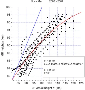
These data are shown in Fig. 3, simply presenting MR (real) heightshvs. LF virtual heightsh′, and a quadratic fit is added. Note that this fit was not produced by forcing the line to pass through some selected point, but the regression shows that – on a long-term average – the group retardation is negligible below 81 km. At greater heights, it may result in an overestimation of the height by up to 20 km. Owing to the
Fig. 3. Real heights observed by MR vs. LF virtual heights for November–March. The blue line representsh′=h, while the black line is calculated by a 2nd order least-squares fit.
small phase shift with height during summer (Fig. 1g, h), the described method can only be applied for the data collected during the winter months. Therefore the correction is, strictly speaking, only valid for November–March, however, as one may see from the following Figs. 4–7, leads to reasonable results for each month including the summer ones.
Fig. 4. Winter (December–February) and summer (June–August) mean zonal prevailing wind (left panel), meridional prevailing wind (middle panel) and semidiurnal amplitude (right panel) as measured by LF without (dashed blue/red) and after virtual height correction (solid blue/red)and by MR (solid black/magenta).
Table 1.Results of a linear best-fit analysis of wind parameters measured by LF vs. MR according tovLF=a+b×vMRbefore (respective upper row) and after (respective lower row) virtual height correction. For the SDT the interceptais set to zero. Correlation coefficientsrare also added. In the table “winter” refers to November–March and “summer” refers to May–September.
Zonal prevailing wind Meridional prevailing wind SDT tidal amplitude
Height Season a b r a b r a b r
85 km Year −4.55 1.39 0.57 −0.35 0.88 0.56 − 0.64 0.35
−0.23 0.75 0.68 −2.14 0.58 0.60 0.58 0.46
85 km Winter 7.22 0.28 0.14 −2.46 1.21 0.26 − 0.28 0.49 6.83 0.21 0.28 −2.96 0.77 0.45 0.30 0.74 85 km Summer −10.70 1.28 0.65 0.84 1.39 0.67 − 0.85 0.29
−3.92 0.76 0.69 4.31 0.99 0.73 0.77 0.46
88 km Year −0.74 0.50 0.31 −1.42 0.78 0.57 − 0.45 0.22 2.01 0.44 0.83 −3.49 0.44 0.66 0.44 0.57 88 km Winter 6.99 0.21 0.23 −2.64 0.50 0.31 − 0.21 0.49 4.63 0.30 0.61 −3.60 0.60 0.31 − 0.21 0.49
1.45 0.42 0.85 −0.71 0.65 0.74 0.58 0.73
91 km Year 2.44 0.21 0.39 −2.86 0.71 0.58 − 0.32 0.15 1.45 0.56 0.85 −4.18 0.45 0.48 0.37 0.71 91 km Winter 6.34 0.12 0.31 −3.31 0.45 0.39 − 0.19 0.78 2.54 0.50 0.68 −4.85 0.59 0.61 0.31 0.67 91 km Summer −3.65 0.37 0.56 −0.71 0.97 0.72 − 0.61 0.57 2.89 0.49 0.79 −2.77 0.46 0.36 0.48 0.90
Results of linear fits of LF winds vs. MR winds after
vLF=a+b×vMRare presented in Table 1 for different
sea-sons and 3 different heights. Correlation coefficientsr are also given. With few exceptions, correlation coefficients in-crease after height correction, which is valid both for win-ter and for summer. Note that this is also the case for the summer SDT, notwithstanding the long-term mean gradient differences between LF and MR. Correlation coefficients for the zonal prevailing wind are generally larger for summer than for winter, which is due to the small mean gradients in
340 C. Jacobi: Meteor radar measurements of mean winds and tides over Collm
Fig. 5.LF vs. MR zonal prevailing wind at 85, 88, and 81 km after virtual height correction of the LF data. Linear best fit curves for the whole data set are added. The heavy solid green line denotes y=x.
Fig. 6.As in Fig. 4, but for the meridional prevailing wind.
while after virtual height correction the slope increases for winter, it decreases for summer, the later being the effect of the different sign of the vertical gradients.
5 Mean wind and SDT amplitude comparison after height correction
Figs 1 and 4 show that, in addition to the height difference, LF measurements underestimate the winds with respect to the MR. The height-corrected LF zonal prevailing winds for 3 radar height gates are shown in Fig. 5, together with linear regression results afterv0z,LF=a+b×v0z,MR(see also
Ta-ble 1). Solid symbols show winter (November–March here) data. LF underestimation is somewhat weaker in the
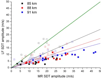
lower-Fig. 7.As in Fig. 4, but for the SDT amplitude. The linear fits were performed with prescribing the intercept asa=0.
most height gate considered, however, one has to take into account that some of the strong westward winds at 85 km in summer may be a result of extrapolation if there are few LF data only, so that the slope (coefficientb) may be slightly too small. Otherwise the summer data do not stand out against the other ones so that one may use the wind LF height cor-rection during the whole year as a first approximation.
The meridional component (Fig. 6) is underestimated by LF in a similar manner as the zonal one, but the corre-spondence is generally worse, and the underestimation even stronger, an effect that has already been noted by Jacobi et al. (2009). Also, the intercept of the regression lined differs somewhat from zero. As is the case with the zonal wind, there is no clear height effect visible.
6 Discussion and conclusions
An overlap of about three years of MR and LF wind mea-surements in the MLT allows the analysis of necessary vir-tual height correction of LF reference heights as well as the estimation of LF mean wind and SDT amplitude underesti-mation. The virtual height effect is small near 80 km, but increases to more than 20 km difference between virtual and real height at 120 km virtual height. The virtual height cor-rection is performed using an empirical statistical approach. In future study, empirical D region electron densities from the IRI model (Bilitza, 2001; Bilitza and Reinisch, 2008) should be considered for a more physical approach, but it has to be taken into account that the data base for the D-region in the IRI model is small and thus IRI results are uncertain as well.
The analysis of LF winds has to be carried out assuming circularly polarized SDT components. Analysis of monthly mean tidal parameters using the MR measurements without assuming circular polarization lead to a mean phase differ-ence of 2.94±0.57 h and a zonal-meridional amplitude dif-ference of -0.52±2.87m/s, confirming earlier results using other midlatitude radars (Jacobi et al., 1999). Thus, the ap-plied LF phase determination is justified. This, however, is only proved for the latitude range considered. At other lati-tudes, phase polarization may be different at least during part of the year (e.g., Zhao et al., 2005).
The LF winds generally underestimate the MR ones by about 50%. The effect is broadly independent of height for the prevailing wind, but increase with height for the SDT amplitudes. It has to be taken into account, however, that the mean winds are generally weaker than the SDT amplitudes, and clearer effects may be masked by the general variability. The reason for wind underestimation by LF is not fully un-derstood. It may be an indirect effect of gravity waves, which may provide some signature in a spaced receiver analysis as is employed by the LF measurements. A similar effect is seen in MF winds (Manson et al., 2004; Jacobi et al., 2009). Since gravity wave activity minimizes around the equinoxes (e.g., Placke et al., 2011), this may also explain the weaker effect on late summer SDT amplitudes.
Acknowledgements. This study was supported by Deutsche Forschungsgemeinschaft under grant JA 836/22-1.
Topical Editor Matthias F¨orster thanks Jens Taubenheim and Dora Pancheva for their help in evaluating this paper.
References
Bilitza, D.: International Reference Ionosphere 2000, Radio Sci., 36, 261–275, 2001.
Bilitza, D. and Reinisch, B.: International Reference Ionosphere 2007: Improvements and new parameters, Adv. Space Res., 42, 599–609, 2008.
Groves, G. V.: A theory for determining upper-atmosphere winds from radio observations on meteor trails, J. Atmos. Terr. Phys., 16, 344–356, 1959.
Hall, C. M., Aso, T., Tsutsumi, M., Nozawa, S., Manson, A. H., and Meek, C. E.: A comparison of mesosphere and lower thermosphere neutral winds as determined by meteor and medium-frequency radar at 70◦N. Radio Sci., 40, RS4001, doi:10.1029/2004RS003102, 2005.
Hocking, W. K. and Thayaparan, T.: Simultaneous and collocated observations of winds and tides by MF and meteor radars over London, Canada (43◦N, 81◦W), during 1994–1996, Radio Sci., 2, 833–865, 1997.
Hocking, W. K., Fuller, B., and Vandepeer, B.: Real-time deter-mination of meteor-related parameters utilizing modern digital technology, J. Atmos. Solar-Terr. Phys., 63, 155–169, 2001. Jacobi, C., Portnyagin, Y. I., Solovjova, T. V., Hoffmann, P., Singer,
W., Fahrutdinova, A. N., Ishmuratov, R. A., Beard, A. G., Mitchell, N. J., Muller, H. G., Schminder, R., K¨urschner, D., Manson A. H., and Meek, C. E.: Climatology of the semidi-urnal tide at 52◦N–56◦N from ground-based radar wind mea-surements 1985–1995, J. Atmos. Solar-Terr. Phys., 61, 975–991, 1999.
Jacobi, C., Arras, C., K¨urschner, D., Singer, W., Hoffmann, P., and Keuer, D.: Comparison of mesopause region meteor radar winds, medium frequency radar winds and low frequency drifts over Germany, Adv. Space Res., 43, 247–252, 2009.
Jacobi, C. and K¨urschner, D.: Long-term trends of MLT region winds over Central Europe, Phys. Chem. Earth, 31, 16–21, 2006. K¨urschner D.: Ein Beitrag zur statistischen Analyse hochatmo-sph¨arischer Winddaten aus bodengebundenen Messungen, Z. Meteorol., 41, 262–266, 1991.
K¨urschner, D. and Schminder, R.: High-atmosphere wind profiles for altitudes between 90 and 110 km obtained from D1 LF mea-surements over central Europe in 1983/1984, J. Atmos. Terr. Phys., 48, 447–453, 1986.
K¨urschner, D., Schminder, R., Singer, W., and Bremer, J.: Ein neues Verfahren zur Realisierung absoluter Reflex-ionsh¨ohenmessungen an Raumwellen amplitudenmodulierter Rundfunksender bei Schr¨ageinfall im Langwellenbereich als Hilfsmittel zur Ableitung von Windprofilen in der oberen Mesopausenregion, Z. Meteorol., 37, 322–332, 1987.
K¨urschner, D. and Jacobi, C.: The mesopause region wind field over Central Europe in 2003 and comparison with a long-term climatology, Adv. Space Res., 35, 1981–1986, 2005.
Manson, A. H., Meek, C. E., Hall, C. M., Nozawa, S., Mitchell, N. J., Pancheva, D., Singer, W., and Hoffmann, P.: Mesopause dynamics from the scandinavian triangle of radars within the PSMOS-DATAR Project, Ann. Geophys., 22, 367–386, doi:10.5194/angeo-22-367-2004, 2004.
Placke, M., Hoffmann, P., Becker, E., Jacobi, C., Singer, W., and Rapp, M.: Gravity wave momentum fluxes in the MLT – Part II: Meteor radar investigations at high and midlatitudes in comparison with modeling studies, J. Atmos. Solar-Terr. Phys., doi:10.1016/j.jastp.2010.05.007, 2011.
Stober, G., Jacobi, C., Fr¨ohlich, K., and Oberheide, J.: Meteor radar temperatures over Collm (51.3◦N, 13◦E). Adv. Space Res., 42, 1253–1258, 2008.