Video transition identification
based on
2D
image analysis
Silvio Jamil Ferzoli Guimar˜aes
Video transition identification based on
2D
image
analysis
This text corresponds to the Thesis which is
pre-sented by Silvio Jamil Ferzoli Guimar˜aes and
ap-preciates by Jury.
Belo Horizonte-Brasil, 14 March 2003 .
Prof. Dr. Arnaldo de Albuquerque Ara´ujo
(Advisor)
Thesis presented to the Departamento de Ciˆencia
da Computa¸c˜ao, ufmg, as a partial requeriment
Departamento de Ciˆencia da Computa¸c˜ao
Universidade Federal de Minas Gerais
Video transition identification based on
2
D
image
analysis
Silvio Jamil Ferzoli Guimar˜
aes
14 March 2003
Jury:
Prof. Dr. Arnaldo de Albuquerque Ara´ujo (Advisor)
DCC-UFMG
Prof. Dr. Michel Couprie (Co-advisor)
ESIEE-FRANCE
Prof. Dr. Neucimar Jerˆonimo Leite (Co-advisor)
IC-UNICAMP
Prof. Dr. Roberto de Alencar Lotufo
FEEC-UNICAMP
Prof. Dr. Jacques Facon
PUC-PR
Prof. Dr. M´ario Fernando Montenegro Campos
DCC-UFMG
Prof Dr. Rodrigo Lima Carceroni
Departamento de Ciˆencia da Computa¸c˜ao
Universidade Federal de Minas Gerais
Identifica¸c˜
ao de transi¸c˜
oes em v´ıdeo baseada na
an´
alise de imagens
2
D
Silvio Jamil Ferzoli Guimar˜
aes
14 de Mar¸co de 2003
Banca:
Prof. Dr. Arnaldo de Albuquerque Ara´ujo (Orientador)
DCC-UFMG
Prof. Dr. Michel Couprie (Co-orientador)
ESIEE-France
Prof. Dr. Neucimar Jerˆonimo Leite (Co-orientador)
IC-UNICAMP
Prof. Dr. Roberto de Alencar Lotufo
FEEC-UNICAMP
Prof. Dr. Jacques Facon
PUC-PR
Prof. Dr. M´ario Fernando Campos Montenegro
DCC-UFMG
Prof. Dr. Rodrigo Lima Carceroni
Universit´e de Marne-la-Vall´ee
Identification de transitions dans des s´
equences
d’images vid´
eo bas´
ee sur l’analyse d’images
2D
Silvio Jamil Ferzoli Guimar˜
aes
14 Mars 2003
Jury:
Prof. Dr. Neucimar Jerˆonimo Leite (Pr´esident)
IC-UNICAMP-Br´esil
Prof. Dr. Arnaldo de Albuquerque Ara´ujo (Directeur)
DCC-UFMG-Br´esil
Prof. Dr. Michel Couprie (Co-directeur)
ESIEE-France
Prof. Dr. Roberto de Alencar Lotufo (Rapporteur)
FEEC-UNICAMP-Br´esil
Prof. Dr. Sylvie Philipp-Foliguet (Rapporteur)
c
Silvio Jamil Ferzoli Guimar˜aes, 2003.
All right reserved.
Aos meus pais, Luiz e Saada, e `a minha amada esposa, Tatiane.
Agradecimentos (in portuguese and
in french)
`
A Deus, por ter me dado sa´ude e coragem para enfrentar este desafio.
Aos meus pais, Luiz e Saada, pelas imensas horas de conforto e
sabedo-ria a mim dispensados dando-me for¸ca para continuidade.
Ao Prof. Arnaldo e ao Prof. Neucimar, pela ajuda, companheirismo e
pelas brilhantes id´eias que foram determinantes para o t´ermino deste
trabalho. N˜ao podendo esquecer tamb´em da ajuda referente as
infini-tas corre¸c˜oes de artigos.
Je remercie `a Michel Couprie pour tant m’aider pendant mon sejour
en France, avec beaucoup de patience et compr´ehension car je ne suis
pas expert de la langue fran¸caise. Je le remercie aussi pour ses id´ees
et pour les discussions toujours int´eressantes.
Ao grupo de trabalho do NPDI do DCC-UFMG, em especial ao Paulo
e ao Camillo. E tamb´em, ao grupo de trabalho do LA2SI-ESIEE, em
especial `a Yukiko, ao Nivando, ao Christophe e ao Marco pelas diversas
discuss˜oes que s´o levaram ao crescimento pessoal e profissional.
Aos meus amigos e colegas do DCC, em especial ao pessoal da minha
turma, Lucila, Mark, F´atima, Maria de Lourdes e, de novo, Paulo.
Aos meus pais, ao CNPq e `a CAPES pelo imprescind´ıvel apoio
finan-ceiro durante toda a minha jornada .
“Eu n˜ao me envergonho de corrigir e mudar minhas opini˜oes, porque
n˜ao me envergonho de raciocinar e aprender.”
(Alexandre Herculano)
Abstract
The video segmentation problem consists in the identification of the boundary between
consecutive shots in a video sequence. The common approach to solve this problem is
based on the computation of dissimilarity measures between frames. In this work, the
video segmentation problem is transformed into a problem of pattern detection, where
each video event is represented by a different pattern on a 2D spatio-temporal image,
called visual rhythm. To cope with this problem, we consider basically morphological and
topological tools that we use in order to identify the specific patterns that are related
to video events such as cuts, fades, dissolves and flashes. To compare different methods
we define two new measures, the robustness and the gamma measures. In general, the
proposed methods present the quality measures better than the other methods used to
comparison.
R´
esum´
e
Le probl`eme de la segmentation de s´equences d’images vid´eos est principalement associ´e
au changement de plan. L’approche courante pour r´esoudre ce probl`eme est bas´ee sur
le calcul de mesures de dissimilarit´es entre images. Dans ce travail, le probl`eme de la
segmentation de s´equences vid´eo est transform´e en un probl`eme de d´etection de motifs,
o`u chaque ´ev`enement dans la vid´eo est represent´e par un motif diff´erent sur une image
2D, apell´ee rythme visuel. Cette image est obtenue par une transformation sp´ecifique
de la vid´eo. Pour traiter ce probl`eme, nous allons consid´erer principalement des outils
morphologiques et topologiques. Nous montrons commment identifier grˆace `a ces outils,
les motifs sp´ecifiques qui sont associ´es `a coupures, fondus et fondus enchaˆın´es, ainsi qu’aux
flashs. Dans l’ensemble, les m´ethodes propos´ees dans cette th`ese obtiennent des indices
de qualit´e meilleurs que les autres m´ethodes auxquelles nous les avons compar´ees.
Resumo
O problema de segmenta¸c˜ao em v´ıdeo consiste na identifica¸c˜ao dos limites entre as tomadas
em um video. A abordagem cl´assica para resolver este problema ´e baseada no c´alculo de
medidas de dissimilaridade entre quadros. Neste trabalho, o problema de segmenta¸c˜ao
em v´ıdeo ´e transformado em um problema de detec¸c˜ao de padr˜oes, onde cada evento de
v´ıdeo ´e transformado em diferentes padr˜oes em um imagem espa¸co-temporal 2D, chamada
ritmo visual. Para tratar este problema, n´os consideramos basicamente ferramentas
mor-fol´ogicas e topol´ogicas com o objetivo de identificar os padr˜oes espec´ıficos que s˜ao
rela-cionados `a eventos do v´ıdeo, como cortes, fades, dissolves e flash. Para comparar os
diferentes m´etodos, n´os definimos duas novas medidas de dissimilaridade, a robusteza
e a medida gama, que relacionam as medidas b´asicas de qualidade com um fam´ılia de
limiares. Os resultados obtidos a partir dos m´etodos propostos, definidos em termos de
medidas de qualidade, s˜ao melhores que os resultados dos outros m´etodos usados como
crit´erio de compara¸c˜ao.
Contents
Agradecimentos (in portuguese and in french) vii
Abstract ix
R´esum´e x
Resumo xi
List of Definitions xvi
List of Figures xviii
1 Introduction 1
1.1 Our contribution . . . 3
1.2 Organization of the text . . . 4
I
Theoretical background
6
2 Video model 7 2.1 Basic definitions . . . 72.2 Types of transitions . . . 9
2.2.1 Cut . . . 10
2.2.2 Fade . . . 10
2.2.3 Dissolve . . . 11
2.2.4 Wipe . . . 12
2.2.5 Transition classification . . . 12
2.3 Camera work . . . 13
2.4 Conclusions . . . 13
3 Video analysis 15 3.1 Video segmentation . . . 16
3.1.1 Approaches based on dissimilarity measures . . . 16
3.1.2 Image-based . . . 20
3.2 Camera work analysis . . . 20
3.3 Quality measures for video analysis . . . 22
3.3.1 Quantitative analysis . . . 22
3.3.2 Threshold sensitivity . . . 23
3.4 Conclusions . . . 25
4 Video transformation from 2D+t to 1D+t 26 4.1 Visual rhythm by sub-sampling . . . 26
4.1.1 Pattern analysis . . . 27
4.2 Visual rhythm by histogram . . . 32
4.2.1 Pattern analysis . . . 34
4.3 Conclusions . . . 36
II
Video transition identification by
2
D
analysis
37
5 Introduction for video transition identification 38 5.1 Description of the corpora . . . 406 Image analysis operators 41 6.1 Mathematical morphology . . . 41
6.1.1 Basic operators . . . 41
6.1.2 Morphological residues . . . 43
6.1.3 Multi-scale gradient . . . 44
6.2 Thinning . . . 47
6.3 Max-tree . . . 49
6.4 Conclusions . . . 51
7 Cut detection 52
7.1 Introduction . . . 52
7.2 Our method . . . 53
7.3 Experiments . . . 57
7.4 Conclusions and discussions . . . 64
8 Flash detection 66 8.1 Introduction . . . 66
8.2 Based on top-hat filtering . . . 67
8.3 Based on max tree filtering . . . 71
8.4 Experiments . . . 73
8.5 Conclusions and discussions . . . 74
9 Gradual transition detection 76 9.1 Introduction . . . 76
9.2 Method based on multi-scale gradient . . . 77
9.2.1 Transition detection . . . 78
9.2.2 Experiments . . . 82
9.2.3 Analysis of results and parameters . . . 84
9.3 Sharpening by flat zone enlargement . . . 87
9.3.1 Transition detection . . . 89
9.3.2 Experimental analysis . . . 96
9.3.3 Analysis of the results . . . 97
9.4 Conclusions and discussions . . . 98
10 Specific fade detection 100 10.1 Introduction . . . 100
10.2 Video transformation . . . 101
10.3 Analysis based on discrete line identification . . . 101
10.4 Experiments . . . 106
10.5 Conclusions and discussions . . . 107
11 Conclusions and future work 110
Bibliography 113
List of Definitions
2.1 Frame . . . 7
2.2 Video . . . 7
2.3 Shot [4] . . . 8
2.4 Scene [4] . . . 9
2.5 Key-frame . . . 9
2.6 Transition . . . 9
2.7 Cut (sharp transition) . . . 10
2.8 Fade-out . . . 10
2.9 Fade-in . . . 11
2.10 Dissolve . . . 11
2.11 Horizontal wipe . . . 12
2.12 Vertical wipe . . . 12
3.1 Recall, error and precision rates . . . 23
3.2 Robustness . . . 23
3.3 “Missless” error . . . 24
3.4 “Falseless” recall . . . 24
3.5 Gamma measure . . . 25
4.1 Visual rhythm [17] or spatio-temporal slice [57] . . . 27
4.2 Visual rhythm by histogram (VRH) . . . 33
6.1 Morphological gradient [68, 63] . . . 41
6.2 White top-hat [68, 63] . . . 42
6.3 Inf top-hat [68, 63] . . . 42
6.4 Ultimate erosion [68, 63] . . . 42
6.5 Morphological residues [54] . . . 43
6.6 Residue mapping [47] . . . 43
6.7 Soille’s morphological gradient [68] . . . 44
6.8 Gradient based on ultimate erosion . . . 45
6.9 Gradient based on thinning . . . 47
9.1 Flat zone, k-flat zone and k+-flat zone . . . 87
9.2 Transition . . . 87
9.3 Constructible transition point . . . 88
9.4 Destructible transition point . . . 88
10.1 Histogram width . . . 101
List of Figures
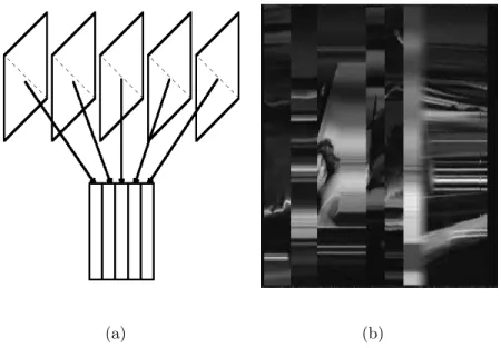
1.1 Video transformation: (a) simplification of the video content by
transfor-mation of each frame into a column on VR; (b) a real VR, obtained by the
principal diagonal sub-sampling (Chapter 4). . . 3
1.2 General framework for our approach to the video segmentation problem. . 4
2.1 Video hierarchical representation [61]. . . 8
2.2 Cut example. . . 10
2.3 Example of fade-out. . . 11
2.4 Example of dissolve. . . 11
2.5 Example of a horizontal wipe (right to left). . . 12
2.6 Example of a vertical wipe (down to up). . . 12
2.7 Camera basic operations. . . 14
2.8 Example of zoom-in. . . 14
3.1 Two different approaches for video segmentation. . . 17
3.2 Video transformation: (a) simplification of the video content by transfor-mation of each frame into a column on VR; (b) a real example of the principal diagonal sub-sampling. . . 21
3.3 Robustness (µ) measure. . . 24
4.1 Example of pixel samplings: D1 is the principal diagonal, D2 is the sec-ondary diagonal, V is the central vertical line and H is the central horizontal line. . . 27
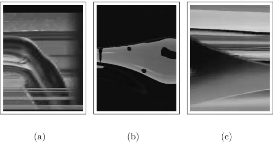
4.2 Examples of visual rhythm by principal diagonal sub-sampling: (a) video “0132.mpg”; (b) video “0599.mpg” and (c) video “0117.mpg”. . . 28
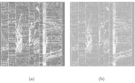
4.3 Visual rhythm obtained by a real video using different pixel sub-samplings:
principal diagonal (top) and central vertical line (bottom). The temporal
positions of the cuts are indicated in the middle image. . . 29
4.4 Block diagram for video segmentation using visual rhythm by sub-sampling. 30
4.5 Examples of sharp transitions in the visual rhythm by sub-sampling (a-c)
vertical sharp transitions, and (d) inclined sharp transition. . . 31
4.6 Examples of gradual transitions present in the visual rhythm. . . 31
4.7 Examples of light and thin vertical regions present in the visual rhythm. . 31
4.8 Example of deformed regions present in the visual rhythm: (a) shifted
re-gion (pan); (b) expanded rere-gion in); and (c) funneled rere-gion
(zoom-out). . . 32
4.9 Real examples of visual rhythm by histogram: (a) video “0094.mpg”; (b)
video “0136.mpg”; (c) video “0132.mpg” and (d) video “0131.mpg”. . . 33
4.10 Block diagram for video segmentation using visual rhythm by histogram. . 34
4.11 Real examples of sharp transitions present in the visual rhythm by histogram. 35
4.12 Examples of orthogonal discontinuities present in visual rhythm by
his-togram. Both contain flashes. . . 35
4.13 Examples of deformed regions present in the visual rhythm by histogram:
(a) corresponds to a fade and (b) to a dissolve. . . 36
5.1 Block diagram for event detection from (a) visual rhythm by sub-sampling
and (b) by histogram in which we are interested. . . 39
6.1 Soille’s gradient. . . 45
6.2 Morphological multi-scale gradient: (a) original 1D image; (b,d,f)
corre-spond to the gradient values at a specific leveln= 4 and (c,e,g) correspond
to the supremum of the gradient values at different levels (n= [1,5]) . . . 46
6.3 Examples of multi-scale gradients where the SE size is in range [1,7]. These
results correspond to the supremum of gradient values of all levels. . . 48
6.4 1D image thinning example. Dotted line, in (b), represents the original
image (a). . . 49
6.5 Process of max-tree creation [62]: (a) original image; (b) first step of the
process considering the levels 0 and 1; (c) second step considering the levels
0, 1 and 2; and (d) the final tree. . . 50
7.1 Cut example. . . 52
7.2 Cut detection block diagram. . . 54
7.3 Visual rhythm by principal diagonal sub-sampling computed from the video
“132.mpg”. . . 55
7.4 Visual rhythm filtered in which the small components are eliminated: (a)
the original visual rhythm and (b) the result of the morphological filtering
(reconstructive opening followed by a reconstructive closing). The radius
size of the horizontal structuring element is 4. . . 56
7.5 Horizontal gradient image. To facilitate the visualization, we apply an
operator to equalize the image histogram. . . 57
7.6 Thinning operation: (a) the equalized horizontal gradient image and (b)
the result of the thinning. To facilitate the visualization, we apply an
operator to equalize the histogram. . . 58
7.7 Detection of maximum points: (a) the equalized thinning image and (b)
the maximum points. . . 59
7.8 Filtering of the maximum points. . . 59
7.9 Cut detection from a visual rhythm by sub-sampling: (a) visual rhythm;
(b) thinning of the horizontal gradient (equalized); (c) maximum points;
(d) maxima filtering; (e) normalized number of maximum points in the
range [0,255]; (f) detected cuts (white bars) superimposed on the visual
rhythm. . . 60
7.10 Cut detection from a visual rhythm by histogram: (a) visual rhythm; (b)
thinning of the horizontal gradient; (c) maximum points; (d) maxima
fil-tering; (e) normalized number of maximum points in the range [0,255]; (f)
detected cuts (white bars) superimposed on the visual rhythm. . . 61
7.11 Experimental results. . . 62
8.1 Flash model: (a) flash occurrence in the middle of the shot and (b) flash
occurrence in the boundary of the shot. . . 67
8.2 Flash video detection: (a) some frames of a sequence with the flash
pres-ence; (b) visual rhythm by sub-sampling; (c) detected flash. . . 68
8.3 Flash detection block diagram using top-hat filtering. . . 68
8.4 Visual rhythm by principal diagonal sub-sampling computed for video
“0600.mpg”. . . 69
8.5 White top-hat filtering: (a) result of the white top-hat and (b) result of
the histogram equalization of (a). . . 69
8.6 Thinning: (a) result of the thinning and (b) result of the histogram
equal-ization of (a). . . 69
8.7 Detection of maximum points . . . 70
8.8 Maxima image filtering. . . 70
8.9 Detection of flashes in which the flashes are represented by white vertical
column bars: (a) original image with 4 flashes and (b) result of the flash
detection. . . 71
8.10 Flash detection block diagram using max-tree filtering. . . 72
8.11 Visual rhythm by principal diagonal sub-sampling computed from video
“0600.mpg”. . . 72
8.12 Average computation: result of the average of the elements for each column. 72
8.13 Result of the max-tree filtering. . . 73
8.14 Detection of flashes in which the flashes are represented by white vertical
column bars: (a) original image with 4 flashes and (b) result of the flash
detection. . . 73
8.15 Experimental results for flash detection. . . 75
9.1 Example of cut and gradual transitions. . . 77
9.2 Block diagrams for detection of transitions considering multi-scale gradient. 79
9.3 Opening operation: (a) thresholded Soille’s gradient in which the SE is in
the range [1,4] and (b) result of the opening operation using a vertical SE
with size equals 2. . . 80
9.4 Number of non-zero gradient values. . . 80
9.5 Closing operation using a SE of size 3. . . 81
9.6 White top operation using SE of size 5. . . 81
9.7 Thinning operation. . . 81
9.8 Detection of some types of transitions, like cuts, fades and dissolves. . . 82
9.9 Example of multi-scale gradient analysis for transition detection, where
n = 7 for the Soille’s multi-scale gradient and gradient based on ultimate
erosion, and n = [1,7] for the gradient based on thinning: the gradient
computation (a,c,e) and the line profile of the projected image (b,d,f). . . . 83
9.10 Graphics of the quality measures: (a) recall; (b) error and (c) precision. . . 85
9.11 Transition points (constructible and destructible). . . 88
9.12 Example of enlargement of flat zones: an artificial example. . . 90
9.13 An example of visual rhythm with some events (a), and the image obtained
by the sharpening process (b). In (c) and (d) is illustrated their respective
line profile of the center horizontal line of the image. . . 91
9.14 Main steps of the proposed gradual transition detection algorithm for video
images. . . 92
9.15 Example of enlargement of flat zones. . . 93
9.16 Gradual transition detection. . . 95
10.1 An example of fade in: ((a)-left) illustrates the frames 0, 14, 24 and 29 of
a transition with 30 frames and their respective histograms ((a)-right); (b)
visual rhythm by histogram of the fade transition; (c) result of the image
segmentation (thresholding) of (b). . . 102
10.2 Visual rhythm by histogram. . . 103
10.3 Block diagram for the fade detection method . . . 103
10.4 Visual rhythm by histogram computed from the video “voyage.mpg”. . . . 104
10.5 Image segmentation using thresholding (threshold= 1). . . 104
10.6 Visual rhythm filtered: (a) the thresholded visual rhythm and (b) the result
of the morphological filtering (opening followed by a closing). The vertical
size of the structuring element is 13. . . 105
10.7 Morphological gradient and thinning: (a) result of the morphological
gra-dient and (b) result of the thinning applied to the image illustrated in
(a). . . 106
10.8 Example of a curve approximation: (a) edge image and (b) segmentation
of the edge in sub-segments. . . 107
10.9 Fade detection: (a) result of the fade-in detection is superimposed on the
visual rhythm by histogram and (b) result of the fade-out detection is
superimposed on the visual rhythm by histogram. . . 108
10.10Fade detection process: (a) visual rhythm by histogram (VRH) computed
from the video “voyage.mpg”; (b) thresholding; (c) gradient; (d) line
filter-ing result; and (e) result superimposed on the VRH. . . 109
11.1 Example of orthogonal discontinuities present in visual rhythm by
his-togram. Both represent flashes. . . 111
Chapter 1
Introduction
Traditionally, visual information has been stored analogically and indexed manually.
Nowadays, due to the improvements on digitalization and compression technologies,
data-base systems are used to store images and videos, together with their meta-data and
associated taxonomy. Unfortunately, these systems are still very costly.
Meta-data include bibliography information, capture conditions, compression
param-eters, etc. The taxonomy is a hierarchy of subjective classes (people, nature, news) used
to organize image/video in different subjects, such as humor, politic, people, etc. A good
selection of meta-data and taxonomy must incorporate special features of the application
that, in general, represent the first step to create and use a large image/video database.
Obviously, there are many constraints related to the use of these indexes: manual
anno-tation represents a big problem in large databases (time-consuming); the domain of the
application and the personal knowledge bias the choice of these indexes, etc.
Unfortu-nately, the existing indexes are always limited in the sense of capturing the salient content
of an image (“a picture is worth a thousand words”) [11, 14, 44, 3, 7, 20].
Multimedia content analysis and content-based indexing represent together a
promis-ing direction for the above methodology. Many systems that consider image/video queries
based on content have been developed [29, 43, 15, 70, 8, 48, 6]. In the last few years,
progress in image/video searching tools for large database systems has been steady. To
build a query in these tools, one can use sketches, selection of visual features (color,
texture, shape and motion), examples and/or temporal/spatial features.
Concerning video, the indexing problem becomes much more complex, because it
2
involves the identification and understanding of fundamental units, such as, scene and
shots. Fundamental units can be semantically and physically sub-divided. To decrease
the number of items to index, we may consider the semantic units, the scenes, instead of
consider the physical units (shots). However, due to the non-structured format, the size
and the general content of a video, this indexing is non trivial [58, 15, 70]. Therefore,
automatic methods for video indexing are extremely relevant in modern applications, in
which speed and precision of queries are required. An example of the use of this index
is video browsing, where it is necessary to segment a video in fundamental units without
knowing the nature and type of the video [60]. Another video problem is the detection
of specific events, such as the identification of the instant in which a predator attacks its
“prey” in a documentary video [38, 37].
TheWorld Wide Webpresents itself as an enormous repository of information, where
thousands of documents are added, replaced or deleted daily. Among these documents,
there are large image/video collections that are produced by satellite systems, scientific
experiments, biomedical systems, etc.
Thus, the need of efficient systems to process and index the information is
unquestion-able, mainly if we are interested in information retrieval. The most important problem
is associated with the exponential increase of the Internet, and the consequent increase
in the number of duplicated documents. According to [16], 46% of all textual documents
have a duplicate. Considering multimedia documents, the problem is more complicated
because the same documents are spread in several machines around the world to facilitate
download, mainly, due to their size.
The need of video contents analysis tools has led many research groups to tackle this
matter, for which different tools have been proposed. Generally, these tools present the
following processing steps [72]:
• video parsing - temporal segmentation that involves identification of different shots,
and camera operation analysis;
• summarization - simplification of video content to facilitate the video browsing;
• classification and indexing - to facilitate the video retrieval.
Differently from the main works presented in literature, which use dissimilarity
1.1. Our contribution 3
consider the problem of video analysis as an image segmentation task. In other words,
the problem of video segmentation will be transformed into a 2D image segmentation
problem, in which the video content is represented by a 2D image, called visual rhythm
(VR). Informally, each frame is transformed into a vertical line on the VR image, as
illustrated in Fig. 1.1(a). Taking advantage of the fact that each event is represented by
a specific pattern in this image, different methods for video analysis based on 2D image
analysis have been proposed in the literature [71, 17, 57, 36].
(a) (b)
Figure 1.1: Video transformation: (a) simplification of the video content by
transforma-tion of each frame into a column on VR; (b) a real VR, obtained by the principal diagonal
sub-sampling (Chapter 4).
1.1
Our contribution
The general aspects of the video segmentation problem based on 2D image analysis has
been already studied in other works, which involve the use of: statistical methods [17],
texture analysis with Markov models [57], texture analysis with Fourier Transforms [1] and
Hough Transforms [42]. However, the computational cost of these approaches is high, and
most important, their results are not satisfactory. In this work we propose new methods
to solve the problem of video segmentation based on 2D image analysis using pre-existing
tools and developing new tools in the domains of mathematical morphology and digital
1.2. Organization of the text 4
work. Firstly, the video is transformed into 2D images. Operators of image processing
are applied to these images to identify some specific events, like cuts, fades, dissolves and
flashes.
Figure 1.2: General framework for our approach to the video segmentation problem.
In the following, we enumerate the major contributions of our work:
• development of video transition identification methods that present low rates of false
detection and high rates of correct detection [36].
• definition and exploitation of a new transformation of the video content, named
visual rhythm by histogram. After application of this transformation, it is possible
to identify cuts, fades and flashes [31, 36, 33].
• a new approach to identify gradual video transitions. This approach is based on the
application of a sharpening method [35] .
• a specific method to detect fade [33].
• two methods to detect flashes [36].
1.2
Organization of the text
We use some basic concepts of Mathematical Morphology and Digital Topology (for
1.2. Organization of the text 5
Chapter 2 - Video model. We discuss the video model taking into account different types of transitions and camera operations.
Chapter 3 - Video analysis. We present related works, considering two different approaches to tackle the video segmentation problem.
Chapter 4 - Video transformation from 2D +t to 1D +t. We define a video
transformation in which video events are transformed into image patterns.
Chapter 5 - Introduction for video transition identification. We introduce the video transition identification problem. We summarize some patterns in which we are
interested, and also the correspondence between the patterns and the transitions.
Chapter 6 - Image analysis operators. We present and define some basic image operators that will be used in our work.
Chapter 7 - Cut detection. A method for cut detection is presented. It takes ad-vantage of the fact that each video event is transformed into a specific pattern on the
transformed image.
Chapter 8 - Flash detection. Two methods to identify flashes are presented. One method is a variant of the cut detection method (Chapter 7) and the other considers a
new approach based on the filtering of a data structure created from statistical values of
the transformed image.
Chapter 9 - Gradual transition detection. Two methods are used to identify grad-ual transitions. One method considers a natural approach in which a multi-scale analysis
is used. The other method tries to eliminate the gradual transitions by applying a
sharp-ening operator followed by an analysis of the sharp transitions.
Chapter 10 - Specific fade detection. We propose a specific fade detection method. Here, we use a new video transformation that considers the histogram information.
Part I
Theoretical background
Chapter 2
Video model
Video is a medium for storing and communicating information. The two most important
aspects of video are its contents and its production style [39]. The video content is the
information that is being transmitted, and the video production style is associated with
the category of a video, such as commercial, drama, science fiction, etc. In this chapter,
we will define some of the concepts used in literature (like shot, scene and keyframe).
Also, we will present the most popular types of transitions (like cut, dissolve, fade and
wipe) and types of camera works (like zoom and pan).
2.1
Basic definitions
Let A⊂ N2, A={0, ...,H−1} × {0, ...,W−1}, where H and W are the height and the
width in pixels of each frame, respectively.
Definition 2.1 (Frame) A frame ft is a function from A to N where for each spatial
position (x, y) in A, ft(x, y) represents the grayscale value of the pixel (x, y) at time t.
Definition 2.2 (Video) A video V, in domain 2D+t, is a sequence of frames ft and can be described by
V = (ft)t∈[0,duration−1] (2.1)
where durationis the number of frames contained in the video. The number of frames is
directly associated with the frequency and the duration of visualization. Generally, the
2.1. Basic definitions 8
huge amount of information represents a problem for video information storage. Thus,
to facilitate the task, file compression techniques, such MPEG 1, MPEG 2, MPEG 7 and
M-JPEG are normally used. In this work, all videos are compressed in MPEG 1 format.
To obtain information for each frame, we decompress only the specific frame without
decompressing the whole video file. Also, each frame is represented in the RGB (Red,
Green, Blue) color space. To facilitate our analysis, we consider only grayscale images,
in which grayscale values are obtained by a simple operation of averaging of the RGB
values.
A video is typically composed by a large quantity of information that is hard to be
physically or semantically related. This is why there is the need to segment a video.
The video fundamental unit is a shot (defined below) that captures a continuous action
considering the recording by a single camera, where the camera motion (e.g., zoom and
pan) and the object motion are permitted. According to [4], a scene is composed by a
small number of shots. While a shot represents a physical video unit, a scene represents
a semantic video unit. To summarize, a scene is a shot grouping that is composed by a
frame sequence, as illustrated in Fig. 2.1.
Figure 2.1: Video hierarchical representation [61].
2.2. Types of transitions 9
frame sequence.
Definition 2.4 (Scene [4]) A scene is usually composed by a small number of inter-related shots that are unified by similar features and by temporal proximity.
Definition 2.5 (Key-frame) A key-frame is a frame that represents the content of a logical unit, as a shot or scene. This content must be the most representative as possible.
A shot consists of a sequence of frames with no significant change in the frame content.
So, by definition, two consecutive frames belong to the same shot if their content is very
similar (or exactly equal). This is true if ft(x, y) ∼= ft+1(x, y) for all t ∈ [1, duration],
where duration means shot size. To study the behavior of consecutive frames, we will
define a 1D image, g, that consists of pixel values ft(x, y) in a spatial position (x, y) at
each time t.
The shots can be grouped into many ways according to the desired effect. For example,
when we search for a video that transmits the idea of motion, the shots must change
rapidly. After that, we describe the transition types without considering the subjective
and intentional aspects.
2.2
Types of transitions
Usually, the process of video production involves two different steps [39], shooting and
editing, the former is for production of shots and the later is for compilation of the different
shots into a structured visual presentation. This compilation is associated with the type
of transition between consecutive shots.
Definition 2.6 (Transition) All edition effect that permits the passing from one shot to another is called transition. Usually, a transition consists of the insertion of a series
of artificial frames produced by an editing tool.
To facilitate the understanding of transition types, we will introduce some notations.
The shot before a transition is denoted by P and the shot after a transition by Q. P(t)
will represent the frame at time t in shotP. The transition between two shotsP and Q,
denoted by T, begins at timet0 and ends at timet1. A frame T(t) represents a frame at
2.2. Types of transitions 10
The choice of transitions in an editing process is associated with the features and style
of the video. The simplest transitions are cut, dissolve, fade and wipe. These transitions
are usually subdivided into sharp transitions (cuts) and gradual transitions (dissolves,
fades and wipes).
2.2.1
Cut
The simplest transition is the cut, which is characterized by the absence of new frames
between consecutive shots. Fig. 2.2 illustrates an example of the cut.
Definition 2.7 (Cut (sharp transition)) A cut is a type of transition where two consecutive shots are concatenated, i.e., no artificial frame is created and the transition
is abrupt.
Figure 2.2: Cut example.
2.2.2
Fade
According to [7], the fade process is characterized by a progressive darkening of a shot
until the last frame becomes completely black, or inversely. A more general definition is
given by [50], where the black frame is replaced by a monochromatic one. Fades can be
subdivided into two types: fade-in and fade-out.
Definition 2.8 (Fade-out) A fade-out is characterized by a progressive disappearing of the visual content of the shot P. The last frame of a fade-out is a monochromatic frame
G (e.g., white or black). The frames of a fade-out can be obtained by
Tfo(t) =α(t)×G+ (1−α(t))×P(t) (2.2)
where α(t) is a monotonic transformation function that is usually linear and t∈ ]t0, t0+
2.2. Types of transitions 11
Definition 2.9 (Fade-in) A fade-in is characterized by a progressive appearing of the visual content of the shotQ. The first frame of the fade-in is a monochrome frameG (ex.
white or black). The frames of a fade-in can be obtained by
Tfi(t) = (1−α(t))×G+α(t)×P(t) (2.3)
Fig. 2.3 illustrates an example of the fade-out.
Figure 2.3: Example of fade-out.
2.2.3
Dissolve
Inversely to the cut, the dissolve is characterized by a progressive change of a shot P into
a shot Q.
Definition 2.10 (Dissolve) A dissolve is a progressive transition of a shot P to a consecutive shot Q with non-null duration. Each transition frame can be defined by
Td(t) = (1−α(t))×P(t) +α(t)×Q(t) (2.4)
Fig. 2.4 illustrates an example of a dissolve.
2.2. Types of transitions 12
2.2.4
Wipe
The wipe is characterized by a sudden change of pixel values according to a systematic
way of chosing the pixels to be changed. Next, two different kinds of wipe are defined.
Definition 2.11 (Horizontal wipe) In a horizontal wipe between two shots P andQ, a “vertical line” is horizontally shifted left or right subdividing a frame in two parts, where
in one side of this line we have contents of P, and in the other side the new shot Q.
Definition 2.12 (Vertical wipe) In a vertical wipe between two shots P and Q, a “horizontal line” is horizontally shifted up or down subdividing a frame in two parts,
where in one side of this line we have the content of P, and in another side the new shot
Q.
Fig. 2.5 and Fig. 2.6 illustrate the examples of horizontal and vertical wipes,
respec-tively.
Figure 2.5: Example of a horizontal wipe (right to left).
Figure 2.6: Example of a vertical wipe (down to up).
2.2.5
Transition classification
In [39, 22], one can find a classification of different types of transitions considering editing
aspects. The classes of transitions are defined as follows:
2.3. Camera work 13
have a geometric model and the duration of this transition is null. The cut is the only
transition of this class.
Type 2: Spatial class - only the spatial aspect between the two shots is manipulated,
so there is a geometric model and the duration of this transition is not null, but the
duration of a pixel transformation is null. The wipe is an example of this class.
Type 3: Chromatic class - only the color space is manipulated without a geometric
model because the whole image is modified at the same time, and the duration of this
transformation is not null. The fade-in, fade-out and dissolve are examples of this class.
Type 4: Spatio-Chromatic class - both color space and spatial aspect are
manipu-lated. The morphing is a kind of this class.
2.3
Camera work
The basic camera operations [2], as illustrated in Fig. 2.7, include: panning - camera
horizontal rotation; zooming - varying of focusing distance; tracking - horizontal traverse
movement; booming - vertical traverse movement; dollying - horizontal lateral movement;
tilting - vertical camera rotation.
Generally, panning and tilting are used to follow moving objects without changing the
location of the camera. Zooming indicates a change in “concentration” about something.
Tracking and dollying often represent a change in viewing or following moving objects
with a camera motion. Fig. 2.8 illustrates an example of a zoom-in.
2.4
Conclusions
In this chapter, we have shown some transition types used in video editing, like cut,
dissolve and fade. We also have shown the most common camera operations, like zoom
and pan. The choice of the events in the video process creation reflects the target of the
2.4. Conclusions 14
Figure 2.7: Camera basic operations.
Figure 2.8: Example of zoom-in.
transition detection) is an enormous and promising domain of study. In this work, we
Chapter 3
Video analysis
Excellent works can be found in literature which summarize and review the main video
problems and the way to cope with them [53, 12, 72, 7]. In general, the first step in video
analysis is video parsing, which can be divided in:
• video segmentation, which consists in dividing the video in fundamental units
ac-cording to the semantic level considered, like shot, scene, etc;
• camera work analysis, which consists in identifying camera operations, like zoom
and pan;
• key-frame extraction, which consists in identifying the representative frames of each
fundamental unit.
Following the parsing, other tasks can be considered, like classification, summarization
and indexing. Classification is concerned with separating scenes or shots in different
classes. According to [72], summarization is essential in building a video retrieval system
where we need to have compact video representations to facilitate browsing. And finally,
video indexing is fundamental for querying large video databases, where the quality and
speed of responses depend on the video descriptor used in the indexing phase.
Usually, video problems are basically related to the analysis of visual features, such as,
color, texture, shape and motion. In this work, we will review some of the most popular
methods to cope with video segmentation problem and we will describe some quality
measures that can be used to compare different methods related to video parsing.
3.1. Video segmentation 16
3.1
Video segmentation
The video segmentation problem can be considered as a problem of dissimilarity between
images (or frames). Usually, the common approach to deal with this problem is based
on the use of a dissimilarity measure which allows the identification of the boundary
between consecutive shots. The simplest transitions between two consecutive shots are
sharp and gradual transitions [39]. A sharp transition (cut) is simply a concatenation of
two consecutive shots. When there is a gradual transition between two shots, new frames
are created from these shots [39].
In the literature, we can find different types of dissimilarity measures used for video
segmentation, based on different visual features, such as pixel-wise comparison,
histogram-wise comparison, edge analysis, etc. If two frames belong to the same shot, then their
dissimilarity measure should be small, and if two frames belong to different shots, this
measure should be large, but in the presence of effects like zoom, pan, tilt and flash,
this measure can be affected. Hence, the choice of a meaningful measure is essential
for the quality of the segmentation results. Another approach to the video segmentation
problem is to transform the video into a 2Dimage, and to apply image processing methods
to extract specific patterns related to each transition. In Fig. 3.1, we illustrate a diagram
that represents the main approaches for video segmentation which are subdivided into
dissimilarity measures and 2D image analysis. In the next sections we will discuss these
approaches and, also, their features and limitations for video segmentation.
3.1.1
Approaches based on dissimilarity measures
The use of dissimilarity measures is based on the following hypothesis: “Two or more
frames belong to the same shot if their dissimilarity measure is small”. The definition of
dissimilarity measures is a bit fuzzy, and it usually depends on the type of visual feature
used to compare two or more frames. Visual features can be broadly classified into four
3.1. Video segmentation 17
Figure 3.1: Two different approaches for video segmentation.
3.1.1.1 Visual features
In what follows, we describe the visual features and make some important remarks about
the most popular methods for video segmentation.
Color-based. The color information is an important image content component, because it is robust with respect to object distortion, object rotation and object translation [66].
The simplest approach used for video segmentation is based on pixel-wise comparisons
between corresponding pixels in consecutive frames. In [79], a simple technique is defined
to detect a qualitative change in the content between two consecutive frames. The
sensi-bility to camera motion represents a problem of this technique, but this influence can be
minimized by the use of a smoothing filter. Another pixel-wise dissimilarity measure is
associated with the average of the pixel difference between two consecutive frames.
Typically, the image color information is represented by an image histogram [6]. The
image histogram (Hf) with color in the range [0, L −1] is a discrete function p(i) =
ni/n, where i is a color of a pixel, ni is the number of pixel in the image f with color
i, n is the total number of pixels in the image and i = 0,1,2, ..., L − 1. Generally,
p(i) = ni/n represents an estimation of the probability of color occurrence i. Taking
advantage of the global information and the invariance to rotation and translation, some
dissimilarity measures based on histogram can be found in [79, 7, 69, 46], among them, are
the histogram intersection and the histogram difference. Another possibility to use color
information is based on statistical measures. [65] used some measures for cut detection,
3.1. Video segmentation 18
transition from mathematical equations, [26] studied the behavior of gradual transitions,
as fades and dissolves, but his method fails in small transitions (transitions with duration
smaller than 15 frames).
Texture-based. Texture is an important element for the human visual system that helps to provide in a scene the idea of depth and orientation of surfaces. The texture
feature represents a very important descriptor of natural images, and is also related to a
visual pattern with some homogeneity property [19, 24, 40, 18, 21, 51].
Other representations for texture information include Markov random fields, Gabor
transforms and wavelet transforms [49]. For video segmentation based on texture, [73]
used wavelet transform for cut detection.
Shape-based. Shape is an important criterium to characterize objects and it is related to their profile and their physical structures [9, 55, 67, 27, 59]. Its use is more frequent
where the image objects are similar to color and texture, as is the case of medical images.
In image retrieval applications, the shape feature can be considered as global or local.
Some global features are symmetry, circularity and central moments. Local features are
associated with size and segment orientation, curvature points, curve angles, etc.
As for image retrieval, we can use the local features as dissimilarity measures for video
segmentation. Some works consider edge analysis for event detection [75, 76, 77], this
technique is associated with the number of edges that appear and disappear in consecutive
frames, but this method is very costly with respect to computational time due to the
computation of edges for each frame of the sequence. From this method, it is possible to
detect fades, dissolves and wipes.
Motion-based. Motion can be considered the most important attribute of a video. Two approaches can be considered for motion-based video segmentation: blocking matching
and optical flow [41]. The motion-based video segmentation is related to the change of the
motion model in consecutive shots. From this approach, high-level features that reflect
camera motions such as panning, tilting and zooming can be extracted (as we will see in
3.1. Video segmentation 19
3.1.1.2 General frameworks for video segmentation
With the aim of increasing the robustness of the results for video segmentation, some
techniques can be applied to different approaches, i.e., we can apply the same process to
different dissimilarity measures. In the original papers, the presented techniques were
ap-plied only to a specific dissimilarity measure, but we can easily extend to other measures.
So, we will present these techniques without considering specific measures.
Block-comparison [56, 79]. Instead of computing dissimilarity measures directly from all pixels of the image, the images are divided in blocks and these measures are computed
for each pair of blocks in consecutive frames. Afterwards, we perform an analysis of the
number of blocks that present a dissimilarity measure greater than a threshold. This
technique is more robust to local motions and to noise than pixel-wise comparison.
Post-filtering [22, 31]. This technique is based on the filtering of the dissimilarity measures computed on the video. Firstly, the dissimilarity measure is computed.
Sec-ondly, a filter is applied to the 1Dimage (resulting of the computation of the dissimilarity
measure). And finally, a thresholding is applied. This technique can be used to decrease
the number of false detections and to detect some patterns in the 1D image.
Twin-comparison [79]. Considering that in gradual transitions the dissimilarity mea-sures between two transition frames are greater than the dissimilarity meamea-sures of frames
in a same shot, two different thresholds can be considered Tb and Ts. Ts > Tb are set for
cut and gradual transitions, respectively. If a dissimilarity measured(i, i+ 1) between two
consecutive frames satisfies Tb < d(i, i+ 1) < Ts, then potential start frames for gradual
transitions are detected. For every potential frame detected, an accumulated comparison
A(i) = P
d(i, i+ 1) is computed if A(i) > Tb and d(i, i+ 1)< Ts. The end frame of the
gradual transition is declared when the condition A(i)> Ts is satisfied.
Plateau-method [74]. With the objective of detecting gradual transitions, instead of calculating dissimilarity measures between two consecutive frames, these are calculated
between two frames at timet andt+k, wherek depends on the duration of the transition
3.2. Camera work analysis 20
The choice of a framework and dissimilarity measures, depends on the time constraints
and the expected quality of the results. Usually, for cut detection, the methods that use
pixel values and statistical measures are the fastest, but the best results are obtained by
histogram analysis, where both can consider the block comparison and/or post-filtering.
For gradual transitions, the histogram twin-comparison is the most indicated, because the
plateau-method is highly dependent on the maximum duration permitted for a transition.
3.1.2
Image-based
When we work directly on the video, we have to cope with two main problems: the
high processing time and the choice of a dissimilarity measure. Looking for reducing
the processing time and using tools for 2D image segmentation instead of a dissimilarity
measure, we can transform the video into a 2D image (as we will see in Sec. 4).
The image-based approach for video segmentation is based on transforming the video V
into a 2Dimage, called VR, and applying image processing methods on VR to extract the
specific patterns related to each transition. Informally, each frame is transformed into a
vertical line of VR, as illustrated in Fig. 3.2(a). This approach can be found in [71, 17, 57].
[71] defined the X-ray and Y-ray as the result of a video transformation obtained by a
linear image transformation in each axis, and an edge analysis was performed to detect
cuts. They also cited another video transformation based on the intensity histogram,
but it was not well defined and not exploited. [17] defined the visual rhythm and [57]
defined the spatio-temporal slice, both related to the same video transformation and
a sub-sampling of each frame, like the principal diagonal sub-sampling (illustrated in
Fig. 3.2(b)). [17] used statistical measures to detect some patterns, but the number of
false detections was very high. [57] used Markov models for shot transition detection,
but it fails when the contrast is low between textures of consecutive shots. Statistical
measures are used in [17, 23] for cut, wipe, fade and dissolve detection.
3.2
Camera work analysis
Camera operations represent the effects controlled by the camera man with the intention
3.2. Camera work analysis 21
(a) (b)
Figure 3.2: Video transformation: (a) simplification of the video content by
transforma-tion of each frame into a column on VR; (b) a real example of the principal diagonal
sub-sampling.
consider only camera operation presence, such as zooming and panning.
Nowadays, the main direction of research on estimating camera operations is the
optical-flow-based approach which consists of two main steps [52]: computing the optical
flow in a frame and analyzing the optical flow to extract camera operations. According to
[52], this approach has two major faults in practice: it is generally time-consuming and it
may be generally affected by noise, such as unintentional camera vibration and flashlight
presence. With the purpose of eliminating these faults, [52] presented an approach to
extract camera operations based on X-ray and Y-Ray images, and texture analysis, where
the movement can be estimated by investigating the directivity of the textures by 2D
Discrete Fourier Transform. [46] considered the result of the 2D fast Fourier Transform
as an input for a multilayer perceptron neural network, which will detect the camera
operations.
Another method to extract camera operations is presented in [1]. In this method,
called Video Tomography Method (VTM), tomographic techniques are applied to video
motion estimation, allowing the visualization of the structure of motion. The VTM is
3.3. Quality measures for video analysis 22
the X-ray and Y-ray are computed by horizontal and vertical sub-samplings. Afterwards,
an edge filter is applied with the objective of enhancing of the edges, in particular, a
first order derivative is used. Finally, the Hough Transform is applied to extract zoom
and pan. The purpose of this step is to combine the two main stages of the classical
camera operation detection problem, the matching procedure and the estimation process.
[42] used also Hough Transform, but differently from [1], the edge detection step was
eliminated. According to [42], its results for motion detection are better than those
presented in [1].
The utilization of DFT and Hough Transform to detect specific patterns is interesting,
but the parameter analysis is difficult and the computational cost is relatively high.
3.3
Quality measures for video analysis
The increase in the number of methods for video parsing makes the choice between them
very difficult. In order to find the best method, it is necessary to use the same evaluation
criteria for different works. What follows, we describe some of the metrics found in
literature that are used to characterize the video segmentation quality.
Generally, the goal of quality measures is to verify the performance of methods in
detecting different events in the video. An event can involve transitions like cut, dissolve,
wipe and camera operations like zoom, pan and tilt.
In this work, we define two new measures: robustness, which allows one to analyse the
sensitivity of a transition detection method relative to a threshold; and gamma measure,
which sets a compromise between the number of correct and false detections. We also
present a quantitative analysis of the results.
3.3.1
Quantitative analysis
We denote by #Eventsthe number of events (cuts, fades, flashes, etc.), by #Correctsthe
number of events correctly detected, by #F alses the number of detected frames that do
not represent an event and by #M issesthe number of the events that were not detected,
defined by #M isses = #Events−#Corrects. From these numbers we can define two
3.3. Quality measures for video analysis 23
Definition 3.1 (Recall, error and precision rates) The ratio of number of events correctly detected to the number of events is called the recall rate. The ratio of number
of events falsely detected to the number of events is called the error rate. The ratio of
number of events correctly detected to the sum of correctly and falsely detected is called
the precision rate. These rates are given by
α= ##CorrectsEvents (recall) (3.1)
β = ##EventsF alses (error) (3.2)
δ = #Corrects#Corrects+#F alses (precision) (3.3)
3.3.2
Threshold sensitivity
Let τ be the threshold used for transition detection within the range [0,1]. Let α(τ)
and β(τ) be the recall and error, respectively, with respect to a given threshold τ. If we
consider that for each threshold τ we obtain different values forαand β, we can represent
these relations as functions α(τ) and β(τ), respectively. A new measure can be created
to relate ranges in which α and β are adequate, according to the allowed percentages of
misses and false detections.
Definition 3.2 (Robustness) Letα(τ)and β(τ)be the functions that relate the thresh-old to recall and error rates, respectively. Let Pm and Pf be the percentage of miss and
false detection that are allowed. The robustness µ is a measure related to the interval
where the recall and error rates have values smaller than (1−Pm) and Pf, respectively.
This measure is within the range [0,1] and is given by
µ(Pm, Pf) =
α−1(1−P
m)−β−1(Pf) , if α−1(1−Pm)−β−1(Pf)>0
0 , otherwise
(3.4)
whereα−1 andβ−1 are the inverses of the functionsα(τ) andβ(τ), respectively. Here, the
result of the inverse functions is the rate of recall and error that are related to threshold,
respectively. In Fig. 3.3, we illustrate the robustness measure obtained from functionsα(τ)
3.3. Quality measures for video analysis 24
of the graphic illustrated in Fig. 3.3, because it is desired to correctly detect events with
a “small” number of false detections.
Figure 3.3: Robustness (µ) measure.
Next, we define two other measures,Em andRf, that are associated with the absence
of miss and false detection, respectively.
Definition 3.3 (“Missless” error) The missless error Em is associated with the
per-centage of false detection when we have results without miss (a “small ratio” of miss Pm
can be permitted, like 3%). The missless error is given by
Em(Pm) =β(α−1(1−Pm)) (3.5)
Definition 3.4 (“Falseless” recall) The falseless recall Rf is associated with the
per-centage of correct detection when we have results without false detection (a “small number”
of false detection Pf can be permitted, like 1%). The falseless recall is given by
Rf(Pf) = α(β−1(Pf)) (3.6)
When we use methods for video parsing, we expect the recall to be the highest when
error rate is the smallest. To find the best compromise between these two requirements,
we must define a “reward function” by combining α(τ) and β(τ). Since high values ofα
3.4. Conclusions 25
Definition 3.5 (Gamma measure) The gamma measure γ represents the maximal value of the reward function defined above for all possible values of τ:
γ =max{α(τ)×(1−β(τ))|τ ∈[0,1]} (3.7)
The gamma measure could also be defined as the area between the two curves,α and
β, but this measure is not exploited in this work. The quality of the results is associated
with the values of the measures above defined.
To declare that a method A is better than a method B, it is necessary to evaluate
the quality measures defined previously, for example, A is better than B if the values of
robustness, falseless recall and gamma measure ofAare higher than the values ofB, and if
the values of missless error ofAis smaller thanB. If these considerations do not occur for
all measures, then we need to consider the features more important for the application. To
generalize, the highest values of robustness, falseless recall and gamma measure represent
the best results of a method. The lowest values of missless error represent the best results
of a method.
3.4
Conclusions
In this chapter, we enumerated some video problems and we described how we can cope
with these problems. Also, we described some quality measures used in video analysis to
compare different methods.
For the video segmentation, we presented two approaches, dissimilarity-measure-based
and image-based. Due to the problem of choice a dissimilarity measure, and the possibility
of using 2D image segmentation, we will transform the video segmentation problem into
a problem of 2D image segmentation without consider dissimilarity measures (as we will
Chapter 4
Video transformation from
2
D
+
t
to
1
D
+
t
Usually, the shot transition detection is the first step in the process of automatic video
segmentation and it is associated with the detection of a cut and gradual transitions
between two consecutive shots [39]. In this chapter, we transform the video segmentation
problem into a 2Dimage segmentation problem, taking advantage of the observation that
each video event is represented by a specific pattern in this image. We present the main
patterns found in this image making a correspondence with the video events. We also
discuss about the proposed approaches to solve the problem of image segmentation using
morphological and topological tools, without the need of defining a dissimilarity measure
between frames. In this way, we can use a simplification of the video content, called visual
rhythm, where the video segmentation problem, in the 2D+tdomain, is transformed into
a problem of pattern detection, in domain 1D+t. So, we can apply methods of 2D image
processing to identify different patterns on the visual rhythm because each video effect
corresponds to a pattern in this image, for example, each cut is shows up as a “vertical
line” on the visual rhythm.
4.1
Visual rhythm by sub-sampling
The visual rhythm obtained by sub-sampling (or simply visual rhythm) is a simplification
of the video content represented by a 2D image. This simplification can be obtained by a
4.1. Visual rhythm by sub-sampling 27
systematic sampling of points of the video, such as, extraction of points in the diagonal
of each frame.
Definition 4.1 (Visual rhythm [17] or spatio-temporal slice [57]) Let V = (ft)t∈[0,duration−1] be an arbitrary video sequence, in domain 2D+t. The visual rhythm, in
domain 1D+t, is a simplification of the video in which each frame ft is transformed into
a vertical line of the visual rhythm image VR, defined by
VR(t, z) =ft(rx×z+a, ry×z+b)
where z ∈ {0, ...,HV R−1} and t ∈ {0, ..., duration−1}, HV R and duration are,
respec-tively, the height and the width of the visual rhythm, rx and ry are pixel sampling ratios,
a and b are spatial offsets on each frame. Thus, according to these parameters, different
pixel samplings could be considered, for example, if rx = ry = 1 and a = b = 0 and
H = W then we obtain all pixels of the principal diagonal. If rx = 1 and ry = 0 and
a = 0 andb = W/2 then we obtain all pixels of the central horizontal line. If rx = 0 and
ry = 1 and a = H/2 and b = 0 then we obtain all pixels of the central vertical line, etc.
In Fig. 4.1, we show 4 different examples of the pixel samplings.
Figure 4.1: Example of pixel samplings: D1 is the principal diagonal, D2 is the secondary
diagonal, V is the central vertical line and H is the central horizontal line.
4.1.1
Pattern analysis
The choice of a pixel sampling constitutes an important problem since different samplings
4.1. Visual rhythm by sub-sampling 28
appear as different patterns. Unfortunately, depending on the type of visual rhythm,
this correspondence is not a one-to-one relation, i.e., a cut transition corresponds to a
vertical line, but a vertical line is not necessarily a cut. This problem can be solved
by considering visual rhythms obtained at different pixel sampling rates. Afterwards,
a simple intersection operation between these results may be used to correctly identify
sharp video transitions.
(a) (b)
(c)
Figure 4.2: Examples of visual rhythm by principal diagonal sub-sampling: (a) video
“0132.mpg”; (b) video “0599.mpg” and (c) video “0117.mpg”.
Fortunately, in general, we need to use only the visual rhythm obtained by principal
diagonal sampling because the correspondence problem rarely occurs in practice.
Further-more, the visual rhythm represents the best simplification of the video content, according
to [17]. [17] presented different pixel sampling possibilities with their corresponding
4.1. Visual rhythm by sub-sampling 29
is based on a diagonal because it usually contains both horizontal and vertical features.
In Fig. 4.2, we show examples of visual rhythms obtained by the principal diagonal
sub-sampling. Another example of visual rhythm is shown in Fig. 4.3, where we illustrate
two visual rhythms obtained from the same video but with different pixel sampling rates.
In these cases we use the principal diagonal (Fig. 4.3-top) and the central vertical axis
(Fig. bottom) samplings. We can observe that there are “vertical lines” in Fig.
4.3-bottom that do not correspond to a sharp video transition but all sharp video transitions
correspond to “vertical lines” on the visual rhythm.
Figure 4.3: Visual rhythm obtained by a real video using different pixel sub-samplings:
principal diagonal (top) and central vertical line (bottom). The temporal positions of the
cuts are indicated in the middle image.
In Fig. 4.4, we illustrate the correspondence between visual patterns and video events.
Next, we analyse the different kinds of patterns on the visual rhythm by sub-sampling.
Sharp image transitions. The notion of sharp transitions on the visual rhythm de-pends on the human visual perception. For example, in Fig. 4.5, we illustrate vertical
sharp transitions and an inclined sharp transition. According to the type of visual rhythm,
this pattern can be generally associated with cuts and wipes. On the visual rhythm by
principal diagonal sub-sampling, for example, all cuts are represented by vertical
tran-sitions, but some vertical transitions can be related to diagonal wipes. In practice the
correspondence problem is irrelevant because the number of wipes is typically