www.atmos-chem-phys.net/16/11521/2016/ doi:10.5194/acp-16-11521-2016
© Author(s) 2016. CC Attribution 3.0 License.
Case studies of the impact of orbital sampling on stratospheric trend
detection and derivation of tropical vertical velocities: solar
occultation vs. limb emission sounding
Luis F. Millán1, Nathaniel J. Livesey1, Michelle L. Santee1, Jessica L. Neu1, Gloria L. Manney2,3, and Ryan A. Fuller1
1Jet Propulsion Laboratory, California Institute of Technology, Pasadena, California, USA 2New Mexico Institute of Mining and Technology, Socorro, New Mexico, USA
3NorthWest Research Associates, Redmond, Washington, USA
Correspondence to:Luis F. Millán (lmillan@jpl.nasa.gov)
Received: 26 April 2016 – Published in Atmos. Chem. Phys. Discuss.: 9 May 2016 Revised: 16 August 2016 – Accepted: 29 August 2016 – Published: 16 September 2016
Abstract. This study investigates the representativeness of two types of orbital sampling applied to stratospheric temper-ature and trace gas fields. Model fields are sampled using real sampling patterns from the Aura Microwave Limb Sounder (MLS), the HALogen Occultation Experiment (HALOE) and the Atmospheric Chemistry Experiment Fourier Trans-form Spectrometer (ACE-FTS). The MLS sampling acts as a proxy for a dense uniform sampling pattern typical of limb emission sounders, while HALOE and ACE-FTS represent coarse nonuniform sampling patterns characteristic of solar occultation instruments. First, this study revisits the impact of sampling patterns in terms of the sampling bias, as pre-vious studies have done. Then, it quantifies the impact of different sampling patterns on the estimation of trends and their associated detectability. In general, we find that coarse nonuniform sampling patterns may introduce non-negligible errors in the inferred magnitude of temperature and trace gas trends and necessitate considerably longer records for their definitive detection. Lastly, we explore the impact of these sampling patterns on tropical vertical velocities derived from stratospheric water vapor measurements. We find that coarse nonuniform sampling may lead to a biased depiction of the tropical vertical velocities and, hence, to a biased estimation of the impact of the mechanisms that modulate these veloci-ties. These case studies suggest that dense uniform sampling such as that available from limb emission sounders provides much greater fidelity in detecting signals of stratospheric change (for example, fingerprints of greenhouse gas
warm-ing and stratospheric ozone recovery) than coarse nonuni-form sampling such as that of solar occultation instruments.
1 Introduction
Satellite data have provided a wealth of information on the Earth system and have had a profound impact on operational numerical weather forecasting. Unlike ground-based instru-ments or airborne field campaigns, satellite data provide con-tinuous global coverage, which facilitates the study and as-similation of distributions of atmospheric fields, as well as global model evaluation. However, satellite measurements sample continuously changing atmospheric fields only at dis-crete times and locations, depending on the satellite orbit as well as the measurement technique, which can result in a bi-ased depiction of the atmospheric field.
Typically, the impact of orbital sampling has been eval-uated by comparing a raw model field against a satellite-sampled one. For example, many studies have documented sampling errors for rainfall estimates (e.g., McConnell and North, 1987; North et al., 1993; Bell and Kundu, 1995; So-man et al., 1996; Gebremichael and Krajewski, 2005) and brightness temperatures (Engelen et al., 2000; Brindley and Harries, 2003), as well as O3, CO, temperature and a few
O3 and H2O from 16 satellite instruments, including limb
emission sounders, limb scattering sounders, solar occulta-tion instruments and a stellar occultaocculta-tion instrument. They concluded that coarse sampling may introduce significant sampling uncertainties in climatologies, not only through nonuniform spatial sampling but, more importantly, through nonuniform temporal sampling, that is to say, producing re-gional monthly means using measurements that do not cover the entire month. As expected, the sampling bias was found to be the greatest in regions with large natural variability.
In this study we further evaluate the impact of the Aura Microwave Limb Sounder (MLS), the HALogen Occultation Experiment (HALOE) and the Atmospheric Chemistry Ex-periment Fourier Transform Spectrometer (ACE-FTS) sam-pling patterns using the Canadian Middle Atmosphere Model (CMAM). MLS sampling provides a dense uniform pattern, while HALOE and ACE-FTS are representative of coarser solar occultation sampling patterns. We use HALOE and ACE-FTS sampling patterns because they are commonly used solar occultation datasets and, furthermore, because their sampling patterns are significantly different and thus representative of the range of observation patterns obtained by solar occultation instruments.
Our study has two purposes. (1) We expand upon pre-vious studies by quantifying the sampling bias of these in-struments affecting measurements of upper tropospheric and stratospheric temperature and trace gas species. (2) We inves-tigate how differences in data coverage may affect the out-come of two illustrative atmospheric studies: trend detection and quantification of tropical vertical velocities. We assess the differences in the long-term (>30 years) trends in tem-perature, O3and CO estimated using datasets with different
sampling patterns. Also, we characterize the impact of orbital sampling on derived lower-stratospheric tropical vertical ve-locities. These velocities are computed by correlating the lag of the water vapor “tape recorder” signal between adjacent levels (Niwano et al., 2003; Flury et al., 2012; Jiang et al., 2015). As such, they are likely an upper bound on the actual velocity (Schoeberl et al., 2008). These vertical velocities are modulated by the quasi-biennial oscillation (QBO), seasonal cycles and El Niño–Southern Oscillation (ENSO) (e.g., Flury et al., 2013; Neu et al., 2014; Minschwaner et al., 2016).
This paper is organized as follows: Sect. 2 describes the satellite patterns and the model fields used. Section 3 briefly revisits sampling bias estimates, while the impact of sam-pling on the estimation of long-term trends as well as on trend detection is presented in Sect. 4. Section 5 addresses the impact of orbital sampling on derived tropical vertical ve-locities, and Sect. 6 summarizes our results. The results dis-cussed in this study should be considered as example cases. Whether the results shown represent reasonable estimates of the true orbital-sampling-induced artifacts (e.g., in the sam-pling bias, in the inferred magnitude of the trends or in the derived tropical vertical velocities) may also depend on how well the model fields represent the real atmosphere.
2 Data and methodology 2.1 Model fields
CMAM is used as a proxy for the real atmosphere. CMAM is an extension of the Canadian Center for Climate Modeling and Analysis spectral general circulation model. Detailed de-scriptions of its dynamical and chemical schemes are given by Beagley et al. (1997) and de Grandpré et al. (2000), re-spectively. The free-running version of the model has been extensively evaluated and has been shown to agree rela-tively well with observations relevant to chemistry, dynam-ics, transport and radiation (e.g., de Grandpré et al., 2000; Eyring et al., 2006; Hegglin and Shepherd, 2007; Melo et al., 2008; Jin et al., 2005, 2009).
In this study we use output from the CMAM30 Speci-fied Dynamics (SD) simulation in which temperature and winds have been nudged to the ERA-Interim reanalysis. This dataset exploits the vast progress made by reanalyses in rep-resenting the stratospheric circulation (e.g., Dee et al., 2011) and as such can be used to reliably predict the chemical fields. Before nudging the temperature fields, a technique de-scribed by McLandress et al. (2014) was used to remove tem-poral discontinuities in the ERA-Interim upper-stratospheric temperatures that occurred in 1985 and 1998. CMAM30-SD has been shown to have a good representation of strato-spheric temperature, O3, H2O and CH4 (Pendlebury et al.,
2015); it has been used as a transfer function between satel-lite datasets to construct a reliable long-term H2O data record
(Hegglin et al., 2014), and it has been shown to reproduce halogen-induced midlatitude O3loss sufficiently well for
in-vestigation of long-term O3 trends (Shepherd et al., 2014).
The version of CMAM30-SD used here has a horizontal resolution of approximately 3.75◦ latitude by 3.75◦
longi-tude. This resolution (approximately 400 km) is comparable to the horizontal resolution of HALOE, ACE-FTS and MLS, which is limited by the∼500 km limb-viewing path length, and, hence, no smoothing of the model fields is necessary (Toohey et al., 2013). This version has 63 vertical levels up to 0.0007 hPa with a vertical resolution varying from 100 m in the lower troposphere to about 3 km in the mesosphere. Model results for the period between January 1979 and De-cember 2012 are used in this study.
We evaluate the following CMAM30-SD outputs: temper-ature, O3, CH3Cl, H2O, CO, HCl, N2O and HNO3. These
parameters are an intersection of the available CMAM30-SD outputs, the measurements available for MLS and the mea-surements available for ACE-FTS or HALOE.
2.2 Satellite instrument sampling patterns
stud-ies due to their fine vertical resolution, the excellent precision and accuracy of their self-calibrated measurements, and their potential for detecting many species. However, the sparsity of the measurements makes understanding the impact of their sampling crucial.
HALOE was launched on the Upper Atmosphere Research Satellite (UARS) in 1991, and it measured infrared spec-tra across eight broadband and gas filter channels from 2.45 to 10.04 µm for 14 years. It measured vertical profiles of temperature, pressure and several atmospheric trace gases, with as many as 15 sunrise and 15 sunset profiles of these atmospheric parameters observed at a given latitude each day (Russell III et al., 1993). The HALOE sampling sweeps through its full range of latitude coverage, ranging from±80 to ±50◦ depending on the season, over a period of about
1 month. The vertical resolution of this dataset is about 2– 3 km.
ACE-FTS was launched in 2003 and profiles the atmo-sphere by using solar occultation. It measures infrared spec-tra from 2.2 to 13.3 µm (750 to 4400 cm−1) with high spec-tral sampling (0.02 cm−1), which allows the retrieval of tem-perature, pressure and concentration for several dozen at-mospheric trace gases (Bernath et al., 2005). ACE-FTS is focused on high-latitude science, and thus almost 50 % of its approximately 15 sunrise and 15 sunset occultations per day occur at latitudes around 60◦. Global latitude coverage
is achieved over a period of approximately 3 months. The vertical resolution of this dataset is about 3 km.
Aura MLS was launched in 2004 and measures limb mil-limeter and submilmil-limeter atmospheric thermal emission us-ing heterodyne radiometers coverus-ing spectral regions near 118, 191, 240 and 640 GHz and 2.5 THz, from which tem-perature, trace gas concentrations and cloud ice are retrieved. Daily, it covers latitudes from 82◦S to 82◦N with ∼3500 vertical scans providing near-global observations. The verti-cal resolution of this dataset varies among species; O3, H2O
and HCl have a ∼3 km resolution in the stratosphere, and CO, CH3Cl, HNO3and N2O have a 4–8 km resolution in the
stratosphere (Livesey et al., 2015).
To investigate the impact of orbital sampling, the daily model fields are linearly interpolated to the actual latitude and longitude of the satellite measurements. For the sam-pling patterns, we use a typical year of measurement loca-tions. In particular, we use 1994 and 2005 for HALOE and ACE-FTS, respectively; these are the years with the maxi-mum number of measurements on record for each dataset. For MLS, we use 2008 as a representative year. Gaps in the measurements due to instrument problems as well as year-to-year variations due to orbital state changes are not con-sidered in this study. To avoid differences attributed purely to diurnal cycles, all satellite measurements are assumed to be made at 12:00 UT, obviating the need for interpolation in time. Thus, we focus on spatial differences. Given that our focus is on horizontal/temporal sampling, all satellite mea-surements are assumed to have vertical resolution
compara--90 -60 -30 0 30 60 90
-90 -60 -30 0 30 60 90
-90 -60 -30 0 30 60 90
-90 -60 -30 0 30 60 90
J F M A M J J A S O N D -90
-60 -30 0 30 60 90
J F M A M J J A S O N D -90
-60 -30 0 30 60 90
1 3 10 30 100 300 1000 3000
Sample count
Latitude [
o]
MLS
HALOE
J F M A M J J A S O N D
ACE-FTS
2.2 2.6 3.0 3.4 3.8 4.2 4.6 5.0 5.4 5.8
H2O @ 100 hPa [ppmv]
Figure 1.Left: monthly sampling counts for MLS, HALOE and
ACE-FTS, in 4◦latitude bins. Note the nonuniform color bar
in-crements. Right: zonal mean water vapor at 100 hPa as sampled by MLS, HALOE and ACE-FTS for individual days. White regions denote a lack of measurements.
ble to that of CMAM30-SD; however, we want to emphasize that the vertical resolution of these instruments is in general good enough to resolve the model fields. That is, although the impact of the averaging kernels is not addressed in this study, for the parameters studied here a 3 km averaging ker-nel does not significantly affect their values in the upper tro-posphere/stratosphere.
Figure 1 (left) shows monthly sampling counts for each in-strument. MLS has a dense and nearly uniform sampling over latitude and time, while HALOE and ACE-FTS have sparser and less uniform sample densities because they are limited to two measurements per orbit. Figure 1 (right) shows the zonal mean water vapor field at 100 hPa as sampled by each instrument to highlight how much daily variability may be missed by the HALOE and ACE-FTS sampling patterns. The consequences of these contrasting sampling densities are the main motivation for this study. As discussed by Manney et al. (2007), mapping data into vortex-centered coordinate sys-tems such as those based on potential vorticity (PV) or equiv-alent latitude (EqL) may alleviate some of the solar occul-tation sampling density problems for polar processing stud-ies. However, since this study focuses on near-global trends and tropical upwelling velocities, such vortex-centered coor-dinate systems are of very limited utility here.
3 Sampling biases
We evaluate the sampling biases associated with construct-ing monthly zonal means from the raw and satellite-sampled data. The raw or sampled zonal means for a particular lati-tude bin for each pressure level are given by
Zlx= 1 N
X
CMAM30-SD
100.00 10.00 1.00 0.10
MLS HALOE ACE-FTS
160 180 200 220 240 260 T [K]
-60-30 0 30 60
100.00 10.00 1.00 0.10 0.01 1.0 3.0 5.0 7.0 9.0 11.0 O3 [ppmv]
-60-30 0 30 60
100.00 10.00 1.00 0.10 0.01
-60-30 0 30 60 -60-30 0 30 60 -60-30 0 30 60 1.0 3.0 5.0 7.0 9.0 11.0 H2 O [ppmv] Pressure [hPa]
Latitude [o]
Figure 2. January 2005 zonal means as a function of pressure
for temperature, O3and H2O (top to bottom) in 4◦latitude bins.
Left column is raw CMAM30-SD model fields; other columns are CMAM30-SD as sampled by MLS, HALOE and ACE-FTS (left to right), respectively. White regions denote a lack of measurements.
whereN is the total number of points,y, belonging to a lat-itude binlandx is a placeholder variable for either the raw data, denoted by the superscript r, or the sampled data, de-noted by the superscript s. Figure 2 shows examples of raw and sampled zonal means for temperature, O3and H2O. The
difference between the satellite-sampled zonal mean and the raw zonal mean gives the absolute sampling bias, that is to say,
SA=Zls−Zrl (2)
or, in percentage,
SP=
Zls−Zrl
Zlr ×100. (3)
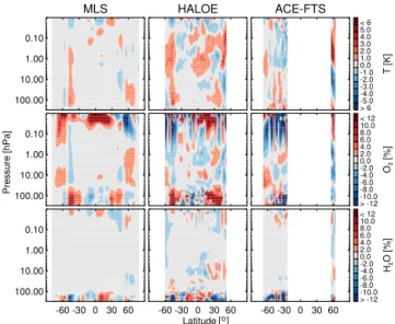
Figure 3 shows examples of the sampling biases for tempera-ture, O3and H2O for January 2005 CMAM30-SD fields.
Rel-ative biases are shown for trace gas species to accommodate their strong vertical gradients. These biases only display the impact of sampling the CMAM30-SD fields; as mentioned before, how well these biases represent the true atmospheric sampling biases will depend on how close the model fields are to the real atmospheric state.
For each month, instrument and pressure level, this bias was computed for all the latitude bins in which an instrument was able to sound the atmosphere. To summarize the poten-tial sampling biases, we computed root-mean-square (RMS) biases over 1 year’s worth of data. As an example, Fig. 4 shows these calculated RMS sampling biases for tempera-ture, O3and H2O for 2005. Overall, there is a direct
corre-lation between the sampling biases and the variability of the
MLS 100.00 10.00 1.00 0.10 HALOE ACE-FTS > 6 -5.0 -4.0 -3.0 -2.0 -1.0 0.0 1.0 2.0 3.0 4.0 5.0 < 6 T [K] 100.00 10.00 1.00 0.10 > -12 -10.0 -8.0 -6.0 -4.0 -2.0 0.0 2.0 4.0 6.0 8.0 10.0 < 12 O3 [%]
-60 -30 0 30 60 100.00
10.00 1.00 0.10
-60 -30 0 30 60 Latitude
-60 -30 0 30 60 > -12 -10.0 -8.0 -6.0 -4.0 -2.0 0.0 2.0 4.0 6.0 8.0 10.0 < 12 H2 O [%] Pressure [hPa]
[o]
Figure 3.January 2005 sampling bias as a function of latitude and
pressure for temperature, O3and H2O (top to bottom) as measured
using MLS, HALOE and ACE-FTS sampling patterns (left to right). White regions denote a lack of measurements.
MLS 100.00 10.00 1.00 0.10 HALOE ACE-FTS 0.00 0.50 1.00 1.50 2.00 2.50 3.00 3.50 4.00 4.50 5.00 5.50 6.00 T [K] 100.00 10.00 1.00 0.10 0.00 1.00 3.00 5.00 10.00 30.00 50.00 100.00 O3 [%]
-60 -30 0 30 60 100.00
10.00 1.00 0.10
-60 -30 0 30 60 Latitude
-60 -30 0 30 60 0.00 1.00 3.00 5.00 10.00 30.00 50.00 100.00 H2 O [%] Pressure [hPa]
[o]
Figure 4.Root-mean-square sampling bias for 2005 as a function
of latitude and pressure for temperature, O3and H2O (top to
bot-tom) as measured using MLS, HALOE and ACE-FTS sampling pat-terns (left to right). White regions denote a lack of measurements.
geophysical parameters. For example, as noted by Toohey et al. (2013), O3sampling biases for the three instruments are
smaller in the tropics and larger at midlatitudes and in the polar regions, where variability is low or high, respectively. However, the biases in all regions are minimized by dense uniform sampling such as that of MLS.
Mean Maximum
0.1 1 10 100
T [K] 100.00
10.00 1.00 0.10 0.01
Pressure [hPa]
0.1 1 10 100
O3 [%]
0.1 1 10 100
CH3Cl [%]
0.1 1 10 100
H2O [%]
0.1 1 10 100
CO [%] 100.00
10.00 1.00 0.10 0.01
Pressure [hPa]
0.1 1 10 100
HCl [%] 0.1 1N2O [%]10 100
0.1 1 10 100
HNO3 [%]
MLS
HALOE
ACE-FTS
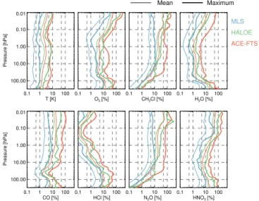
Figure 5. Mean (thin lines) and maximum (thicker lines) RMS sampling bias over all latitudes for 2005 as a function of pressure
for temperature (in Kelvin), O3, CH3Cl, H2O, CO, HCl, N2O and
HNO3in percent. The vertical grid indicates values of 0.5, 1, 5, 10,
50 and 100.
pling biases 1 order of magnitude larger than those of MLS. For example, for the occultation sensors, the temperature maximum sampling biases are about 10 K compared to 1 K for MLS. Similarly, in the middle stratosphere, H2O
maxi-mum sampling biases for the solar occultation instruments can be as large as 5 % compared to less than 1 %, and lastly, HNO3 maximum sampling biases can be as large as 50 %
compared to less than 5 %.
4 Long-term trends
We now evaluate the impact of orbital sampling on the rep-resentation of long-term trends. Accurate reprep-resentation of long-term trends is crucial because they are indicators of climate change, as well as ozone recovery. To summarize the effect of the orbital sampling upon long-term trends we use Taylor diagrams (Taylor, 2001), which provide a conve-nient method for visualizing statistics of how closely patterns match each other; in this case, they are used to depict the suc-cess of the satellite-sampled data in representing the variabil-ity found in the raw model fields. The similarvariabil-ity is quantified by their correlation coefficient, their centered RMS differ-ence (RMSd) and their standard deviations. Simply, the cen-tered RMSd is the RMS of the differences between the two anomaly time series.
In the diagrams shown, all data are normalized to the raw model standard deviation to facilitate showing different pressure levels in the same figure. In these diagrams, there are four things to consider: (1) the azimuth angle indicates the correlation between the satellite-sampled and raw data; (2) the point with normalized standard deviation of 1 and
correlation of 1 is the reference point and corresponds to the raw model data; (3) the distance between any point in the figure and the reference point indicates the ratio of the centered RMSd and the raw model standard deviation (green contours); and (4) the distance between other points in the plot and the origin is the ratio between the satellite-sampled standard deviation and that of the raw model field.
Near-global (60◦S–60◦N) long-term (1979–2012)
pat-terns are compared between satellite-sampled and raw model fields in Fig. 6 for all the atmospheric parameters evaluated in this study. Means were computed by averaging all data avail-able between 60◦N and 60◦S with no effort to use only
lati-tudes where the satellites sampled. This approach was taken to show the representativeness of near-global patterns. We did not expand this study to the latitudes poleward of 60◦N
or 60◦S because ACE-FTS does not sample these areas for 4
months per calendar year and HALOE does not sample for 5 and 6 months at the South and North Pole, respectively (see Fig. 1). Figure 7 shows the raw model standard deviations used to normalize these diagrams (black lines). Overall, the MLS-sampled data (circles in Fig. 6) for all variables and all pressure levels are close to the reference point, indicating high correlation coefficients, low centered RMSd and the ex-pected standard deviation (i.e., a standard deviation similar to that of the full model fields). The HALOE-sampled data (triangles) show intermediate performance, followed by the ACE-FTS-sampled data (squares), which show the weakest correlation and the largest normalized standard deviation. For example, this is easily seen in the CO Taylor diagram, where the MLS-sampled points all cluster tightly at the reference point, whereas HALOE-sampled points lie farther away and ACE-FTS-sampled points the farthest.
To highlight the impact of these sampling differences, Fig. 8 shows trend estimates for near-global temperature at 10 hPa using the raw and satellite-sampled data. Three meth-ods have been used to compute the trends. The first is a sim-ple linear fit (an ordinary least square regression) through the points. In the second, we deseasonalize the data (we re-move the observed climatological monthly mean at every grid point) before computing a linear fit. Lastly, we consider a trend model of the form
Y=µ+ω t
12+S+N, (4)
whereY is the monthly raw or sampled average measure-ments (temperature, CO or O3 concentration, etc.),µ is a
baseline constant,ωis the mean trend per year,t is time in months,Sis a seasonal mean component represented by
S=a1sin(2π
12t+b1)+a2sin( 2π
6 t+b2), (5)
0.00.20.40.60.81.0 0 2 4 6 8 10 MLS HALOE ACE-FTS 0.1 hPa 1.0 hPa 10.0 hPa 100.0 hPa 200.0 hPa 300.0 hPa 0 2 4 6 8 101214
T 0 2 4 6 8 10 12 14 0.0 0.1 0.2 0.3 0.4 0.5 0.6
0.7 0.8
0.9
0.95
1.0
3 6 9 12
0 2 4 6 8 101214
O3 0 2 4 6 8 10 12 14 0.0 0.1 0.2 0.3 0.4 0.5 0.6
0.7 0.8
0.9
0.95
1.0
3 6 9 12
0 2 4 6 8 101214
CH3Cl
0 2 4 6 8 10 12 14 0.0 0.1 0.2 0.3 0.4 0.5 0.6
0.7 0.8
0.9
0.95
1.0
3 6 9 12
0 2 4 6 8
H2O
0 2 4 6 8 0.0 0.1 0.2 0.3 0.4 0.5
0.6 0.7 0.8 0.9 0.95 1.0 1 1 2 3 4 5 6
0 1 2 3
CO 0 1 2 3 0.0 0.1 0.2 0.3 0.4 0.5
0.6 0.7 0.8 0.9 0.95 1.0 1 1
0 1 2 3 4 5
HCl 0 1 2 3 4 5 0.0 0.1 0.2 0.3 0.4 0.5
0.6 0.7 0.8 0.9 0.95 1.0 1 1 2 3
0 1 2 3 4
N2O
0 1 2 3 4 0.0 0.1 0.2 0.3 0.4 0.5
0.6 0.7 0.8 0.9 0.95 1.0 1
1 2
0 1 2 3 4 5
HNO3 0 1 2 3 4 5 0.0 0.1 0.2 0.3 0.4 0.5
0.6 0.7 0.8 0.9 0.95 1.0 1 1 2 3
Norm. standard deviation
Norm. standard deviation
Figure 6.Taylor diagrams showing near-global (60◦S to 60◦N) long-term (1979–2012) pattern comparisons between the raw (the reference point at (1,0)) and the satellite-sampled data at different pressure levels. The green contours indicate the normalized RMS difference values.
0 2 4 6 8 T [K] 100.0 10.0 1.0 0.1 Pressure [hPa]
0.0 0.2 0.4 0.6 O3 [ppmv]
0 5 10 15 CH3Cl [pptv]
0.1 1.0 10.0 H2O [ppmv]
1 10 100 CO [ppbv] 100.0 10.0 1.0 0.1 Pressure [hPa]
0.0 0.1 0.2 0.3 0.4 HCl [ppbv]
0 5 10 15 N2O [ppbv]
0 500 1000 HNO3 [pptv]
30º N–60º N 60º S–60º N
Figure 7. Raw model standard deviations used to normalize the
Taylor diagrams shown in Figs. 6 and 10. Note that H2O and CO
are shown using a logarithmic scale.
N =φN1+ε, (6)
whereφis the autocorrelation of the noise, computed and as-sumed temporally invariant, following Tiao et al. (1990), and
εis independent white noise variables with varianceσε2. As pointed out by Tiao et al. (1990),φhas the effect of reduc-ing the amount of information that would have been avail-able in the same number of independent data points. Similar models have been used in many previous trend studies (e.g. Tiao et al., 1990; Weatherhead et al., 1998; Boers and Mei-jgaard, 2009; Whiteman et al., 2011). As shown in Fig. 8, HALOE (ACE-FTS) sampling artificially reduces (increases) the trend estimates by about 10 % (25 %). Despite agreement on the sign of the trend, these sampling-induced artifacts will compromise the robustness of the derived temperature trends. We computed the trend using different methods in order to emphasize that using models that are more geophysically
re-alistic, such as those that capture the seasonal component, may not have much impact on the estimated trends or, as pointed out by Weatherhead et al. (1998), on the trend sta-tistical properties.
Figure 9 shows how these sampling-induced trend artifacts vary with altitude. To avoid clutter, this figure only shows the differences in trend magnitude computed using Eq. (4), but the ones computed using the other trend detection meth-ods are similar. We show results for temperature, O3and CO
because these parameters exhibit clear trends at most pres-sure levels in the CMAM30-SD simulations and also because overall they can be accurately described by the model given by Eq. (4). For O3 we only use data starting from 2000 to
capture the expected period of O3 recovery. Overall, MLS
sampling allows the estimation of the trend magnitudes to about 1 order of magnitude better than HALOE and ACE-FTS sampling, with accuracy better than 1 % at most pres-sure levels for temperature and CO and better than 10 % for O3.
Figure 9 also shows the estimated number of years re-quired to definitively detect these trends. When using Eq. (4), the number of years,n∗, needed to detect a given trend with
a 95 % confidence level with a probability of 0.90 can be ap-proximated by (Tiao et al., 1990)
n∗=
"
3.3σN
|ω| s
1+φ
1−φ
#2/3
, (7)
which indicates that trend detectability depends on three fac-tors: (1)φ the autocorrelation of the residual between the data points and the trend model computed following Tiao et al. (1990); (2)σN the standard deviation of the residual,
which corresponds to the unexplained variability of the data; and (3) the absolute magnitude of the trend. It is also noted thatσNis related toσεby
σN2= σ
2 ε
79 80 81 82 83 84 85 86 87 88 89 90 91 92 93 94 95 96 97 98 99 00 01 02 03 04 05 06 07 08 09 10 11 12 226
228 230 232
234 CMAM30-SD -0.26 -0.25 -0.25
79 80 81 82 83 84 85 86 87 88 89 90 91 92 93 94 95 96 97 98 99 00 01 02 03 04 05 06 07 08 09 10 11 12 226
228 230 232
234 EMLS -0.26 (0.39 %) -0.25 (0.46 %) -0.25 (0.51 %)
79 80 81 82 83 84 85 86 87 88 89 90 91 92 93 94 95 96 97 98 99 00 01 02 03 04 05 06 07 08 09 10 11 12 226
228 230 232
234 HALOE -0.24 (-8.98 %) -0.23 (-7.33 %) -0.23 (-9.97 %)
79 80 81 82 83 84 85 86 87 88 89 90 91 92 93 94 95 96 97 98 99 00 01 02 03 04 05 06 07 08 09 10 11 12 226
228 230 232
234 ACE-FTS -0.33 (27.27 %) -0.31 (21.70 %) -0.31 (25.04 %)
T [K]
Figure 8.Time series of near-global (60◦S to 60◦N) temperature at 10 hPa for the raw and satellite-sampled data (gray lines). Orange lines display the trend computed using the linear fit, green lines show the climatological seasonal cycle imposed upon a long-term trend and light
blue lines show the model computed using Eq. (4). The trend (K decade−1) computed using each method is specified in each subplot; in
brackets we show the percentage difference in trend magnitude with respect to the trend found using the raw model data.
-1.2 -0.8 -0.4 0.0 T [K decade-1]
100.0 10.0 1.0 0.1
1 10 100 |Difference| [%]
10 100 1000
No. years
-50 0 50 100 150 O3 [ppbv decade-1]
100.0 10.0 1.0 0.1
1 10 100
|Difference| [%] 10 No. years100 1000
0 5 10 15 20 CO [ppbv decade-1]
100.0 10.0 1.0 0.1
1 10 100
|Difference| [%] 10 No. years100 1000
Pressure [hPa]
CMAM30-SD
MLS
HALOE
ACE-FTS
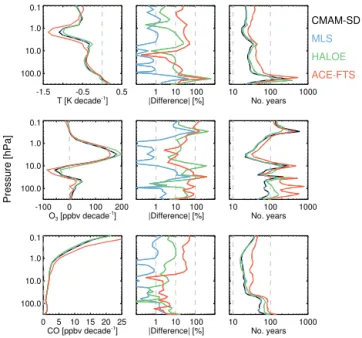
Figure 9.Left: near-global (60◦S to 60◦N) long-term (1979–2012)
trends computed using Eq. (4) for temperature, O3and CO. Middle:
percentage difference in the inferred magnitude of the trends when computed using various satellite-sampled data with respect to the one computed using the raw model fields. Right: number of years required to detect such trends.
in this trend model (Eq. 4). Note that φ was computed for the raw as well as the satellite-sampled data. As shown in Fig. 9, trend detection using data with HALOE or ACE-FTS sampling will require considerably more years than using data with MLS sampling. This is due to an increase in the magnitude ofσNresulting from the noisiness of the time
se-ries based on the HALOE or ACE-FTS sampling patterns
(e.g., Fig. 8). For example, at 1 hPa, the pressure level where the strongest temperature trend is found in CMAM30-SD, a 15-year record of MLS-sampled observations would be re-quired to detect such a trend at the 95 % confidence level, while HALOE and ACE-FTS sampling would require 25 and 30 years, respectively. For O3 at 2 hPa, the pressure level
where the strongest O3trend is found in CMAM30-SD, the
MLS sampling pattern would require about 11 years, while HALOE and ACE-FTS would require about 20 and 30 years, respectively. In addition, MLS sampling requires the same number of years as for the raw model fields; that is, the re-quired number of years is only determined by the natural variability. We also performed this analysis using only the autocorrelation computed for the raw model data and found no significant differences.
We also investigated the effect of instrument noise, using Tiao et al. (1990) and Whiteman et al. (2011):
σN=
s σε2
1−φ2+ σI2
nI, (9)
whereσI is the instrument noise and nI is the number of
mea-0.00.20.40.60.81.0 0 2 4 6 8 10 MLS HALOE ACE-FTS 0.1 hPa 1.0 hPa 10.0 hPa 100.0 hPa 200.0 hPa 300.0 hPa 0.0 0.5 1.0 1.5
T 0.0 0.5 1.0 1.5 0.0 0.1 0.2 0.3 0.4 0.5
0.6 0.7 0.8 0.9 0.95 1.0 0.50 1.00
0.0 0.5 1.0 1.5 O3
0.0 0.5 1.0 1.5 0.0 0.1 0.2 0.3 0.4 0.5
0.6 0.7 0.8 0.9 0.95 1.0 0.50 1.00
0.0 0.5 1.0 1.5 CH3Cl
0.0 0.5 1.0 1.5 0.0 0.1 0.2 0.3 0.4 0.5
0.6 0.7 0.8 0.9 0.95 1.0 0.50 1.00
0.0 0.5 1.0 1.5 H2O
0.0 0.5 1.0 1.5 0.0 0.1 0.2 0.3 0.4 0.5
0.6 0.7 0.8 0.9 0.95 1.0 0.50 1.00
0.0 0.5 1.0 1.5 CO 0.0 0.5 1.0 1.5 0.0 0.1 0.2 0.3 0.4 0.5
0.6 0.7 0.8 0.9 0.95 1.0 0.50 1.00
0.0 0.5 1.0 1.5 HCl 0.0 0.5 1.0 1.5 0.0 0.1 0.2 0.3 0.4 0.5
0.6 0.7 0.8 0.9 0.95 1.0 0.50 1.00
0.0 0.5 1.0 1.5 N2O
0.0 0.5 1.0 1.5 0.0 0.1 0.2 0.3 0.4 0.5
0.6 0.7 0.8 0.9 0.95 1.0 0.50 1.00
0.0 0.5 1.0 1.5 HNO3
0.0 0.5 1.0 1.5 0.0 0.1 0.2 0.3 0.4 0.5
0.6 0.7 0.8 0.9 0.95 1.0 0.50 1.00
Norm. standard deviation
Norm. standard deviation
Figure 10.As Fig. 6 but for 30 to 60◦N.
-1.5 -0.5 0.5 T [K decade-1]
100.0 10.0 1.0 0.1
1 10 100
|Difference| [%] 10 No. years100 1000
-100 0 100 200 O3 [ppbv decade-1]
100.0 10.0 1.0 0.1
1 10 100
|Difference| [%] 10 No. years100 1000
0 5 10 15 20 25 CO [ppbv decade-1]
100.0 10.0 1.0 0.1
1 10 100 |Difference| [%]
10 100 1000
No. years Pressure [hPa] CMAM-SD MLS HALOE ACE-FTS
Figure 11.As Fig. 9 but for 30 to 60◦N.
surements for a given period or aging of the instrument, both of which can induce artificial trends in the data that are not representative of the actual environmental trend studied.
Both HALOE and ACE-FTS provide better coverage in the extratropics than in the tropics (see Fig. 1). Fig-ure 10 therefore shows long-term pattern comparisons be-tween satellite-sampled and raw data for trends derived us-ing only data from 30 to 60◦N. Figure 7 also shows the raw
model standard deviations used to normalize these diagrams (purple lines). In general, HALOE- and ACE-FTS-sampled data correlation coefficients improved considerably over the near-global case, with a correlation coefficient no smaller than∼0.6 and with a centered RMSd better than 1 raw model standard deviation (see Fig. 10). MLS-sampled data are still closest to the reference point. Two variables can have similar trends but still perform poorly in Taylor diagrams due to ei-ther a lack of correlation or different standard deviations. In
both cases, this will impactσN, resulting in an increase in the
number of years required to statistically detect such a trend. Figure 11 is equivalent to Fig. 9 but for the 30 to 60◦N
latitude range. As for the near-global trends, ACE-FTS sam-pling still requires considerably more years to confidently detect a trend than does MLS sampling. HALOE, however, has a more uniform sampling density than ACE-FTS in this latitude range (see Fig. 1), and thus the time required to de-tect a trend is more in line with that for MLS. Nevertheless, MLS sampling allows estimation of trends to about 1 order of magnitude better than HALOE and ACE-FTS sampling. As before, the effect of instrument noise was found to be negligible (for this latitude range the approximate number of measurements in a given month is 19 000, 220 and 70 for MLS, HALOE and ACE-FTS, respectively).
As shown, the ability to detect trends depends upon the natural variability and the correlation of the data. These in turn vary with the specific parameter as well as the location and height being studied. Studies of natural variability and autocorrelation of the data will help identify where to moni-tor to find more readily detectable trends, but such a study is outside the scope of this paper.
5 Tropical vertical velocities
In this section we investigate the impact of orbital sampling upon derived tropical vertical velocities (a key metric for at-mospheric circulation). The vertical velocities are calculated using the same approach as described by Flury et al. (2012) and Jiang et al. (2015). In short, we use time series of daily zonal mean water vapor data averaged between 8◦S and 8◦N
veloc-2000 2001 2002 2003 2004 2005 2006 100
70 50 30 20 10
Pressure [hPa]
-60.0 -48.0 -36.0 -24.0 -12.0 0.0 12.0 24.0 36.0 48.0 60.0
[%]
Figure 12.The atmospheric tape recorder (zonal mean water vapor anomalies in the tropics, in this case for CMAM30-SD raw model fields) displays a clear signal of the large-scale upward transport as indicated by the arrow. The slope of this arrow, which is derived from the propagation speed of the water vapor anomalies, represents
the average tropical upwelling velocity for 8◦S–8◦N. This subset
of years is shown as an example; other years are similar.
ities derived from this method are a measure of the transport velocity averaged over 8◦S–8◦N and have been shown to
agree well with the transformed Eulerian mean residual ver-tical velocity when in-mixing from the extratropics and verti-cal diffusion are small (Schoeberl et al., 2008). Interpolation was used to fill the data gaps due to the sampling patterns. In the case of HALOE sampling, this implies linearly interpo-lating to fill gaps in June and December. For ACE-FTS, gaps are filled in January, March, May, July, September, Novem-ber and DecemNovem-ber, when no measurements are made over the tropics (8◦S to 8◦N); thus, we are applying the analysis to highly interpolated data. Considering the degree of interpola-tion required, we do not recommend the use of ACE-FTS to derive tropical upwelling velocities, but we include this case merely as an illustrative example.
Figure 13 (top) shows the vertical velocities averaged over 60–30 hPa derived using raw model fields as well as the satellite-sampled data. To quantify the impact of the different orbital sampling patterns, Fig. 13 (bottom) displays scatter-plots between the raw fields and the satellite-sampled verti-cal velocities. The best correlation (R=1.00), the best line fit (1.07x+0.02, obtained using an ordinary least squares fit regression) and the smallest RMSd (0.005) are found when using the MLS sampling. ACE-FTS and HALOE sampling lead to non-negligible artifacts when deriving vertical veloc-ities from the tape recorder.
Previous studies have shown variability in middle strato-spheric tropical vertical velocities on the order of up to
±40 % associated with the QBO and ENSO (Flury et al., 2013; Neu et al., 2014; Minschwaner et al., 2016). To better understand the impact of these sampling-induced artifacts, we fit the following model to the monthly vertical velocities
wTR=q·QSI[t−tq] +e·MEI[t−te] +c, (10)
79 81 83 85 87 89 91 93 95 97 99 01 03 05 07 09 11 0.20
0.25 0.30 0.35 0.40 0.45 0.50
w
[mm s ]
TR
CMAM30-SD
MLS
HALOE ACE-FTS
0.2 0.3 0.4 wTR cmam
0.2 0.3 0.4 0.5
wTR
instrument
MLS
RMSD: 0.005 1.07x - 0.02 R: 1.00
0.2 0.3 0.4 wTR cmam
HALOE
RMSD: 0.028 0.79x + 0.07 R: 0.79
0.2 0.3 0.4 wTR cmam
ACE-FTS
RMSD: 0.041 0.81x + 0.05 R: 0.67
-1
Figure 13.Top: wTR(monthly vertical velocities) derived using daily time correlations of the water vapor tape recorder at differ-ent pressure levels from the raw CMAM30-SD data as well as the
satellite-sampled data.wTRderived using the raw model fields and
MLS-sampled data are almost identical. The pressure levels
aver-aged are 30, 40, 50 and 60 hPa. Bottom: wTRscatterplots (mm s−1)
for MLS, HALOE and ACE-FTS sampling, respectively, vs. the ve-locities derived using raw model fields. The slopes’ 95 % confidence
intervals are±0.007, 0.06 and 0.09 for MLS, HALOE and
ACE-FTS, respectively.
where wTR is the vertical velocity derived from the tape
recorder, QSI is a QBO shear index, MEI is the multivariate ENSO index,cis a baseline constant,q andeare constants modifying the magnitude of the QSI or MEI, andtq andte
ACE-79 80 81 82 83 84 85 86 87 88 89 90 91 92 93 94 95 96 97 98 99 00 01 02 03 04 05 06 07 08 09 10 11 0.25
0.35
0.45 (a)
-600 -400 -200 0 200 400
U50-U25
-3 -2 -1 0 1 2 3
MEI
79 80 81 82 83 84 85 86 87 88 89 90 91 92 93 94 95 96 97 98 99 00 01 02 03 04 05 06 07 08 09 10 11 0.25
0.35 0.45
wTR = 1.45E-04*QSI(t-7) +3.33E-03*MEI(t-0) +0.35
(b)
79 80 81 82 83 84 85 86 87 88 89 90 91 92 93 94 95 96 97 98 99 00 01 02 03 04 05 06 07 08 09 10 11 0.25
0.35 0.45
wTR = 1.50E-04*QSI(t-7) +2.96E-03*MEI(t-0) +0.35
(c)
79 80 81 82 83 84 85 86 87 88 89 90 91 92 93 94 95 96 97 98 99 00 01 02 03 04 05 06 07 08 09 10 11 0.25
0.35 0.45
wTR = 1.00E-04*QSI(t-7) +1.21E-03*MEI(t-0) +0.35
(d)
79 80 81 82 83 84 85 86 87 88 89 90 91 92 93 94 95 96 97 98 99 00 01 02 03 04 05 06 07 08 09 10 11 0.25
0.35 0.45
wTR = 9.91E-05*QSI(t-7) -7.63E-04*MEI(t-0) +0.34
(e)
w
[mm s ]
TR
CMAM30-SD
MLS
HALOE
ACE-FTS
-1
Figure 14. (a)Time series ofwTR(mean monthly vertical velocities averaged over 30, 40, 50 and 60 hPa) derived using CMAM30-SD raw data (black), the quasi-biennial oscillation (QBO) shear index (QSI – purple) and the multivariate ENSO index (MEI - orange dashed line).
(b)Time series ofwTRfor the raw model fields (black) as well as the model fit described by Eq. (10) (gray).(c–e)Time series ofwTRfor
satellite-sampled data (color coded). The thin black line displays the samewTRderived using raw model fields (black line inb) for ease of
comparison with the satellite-sampled ones. The model fit for each of the satellite-sampledwTRvalues, described by Eq. (10), is shown in
gray for each of these time series.
FTS sampling underestimate it by 30.7 and 31.5 %, respec-tively. The impact of the sampling is more pronounced for the MEI (the differences ine), with MLS, HALOE and ACE-FTS underestimating its influence by 11, 64 and 122 %. We emphasize that these sampling-induced offsets to the strength of the modulation effects of the QBO and ENSO on the cir-culation are only applicable to CMAM30-SD fields. These fields may not accurately represent the stratospheric tropi-cal vertitropi-cal velocities and, consequently, the actual sampling offsets could be different. As such, they should be considered only as potential biases.
The changes in tropical upwelling associated with QBO and ENSO assessed here have been shown to alter O3
trans-port to the midlatitude lower stratosphere and to account for approximately half the interannual variability in midlati-tude tropospheric O3(Neu et al., 2014). It has been
hypoth-esized that this observed relationship between stratospheric upwelling changes and changes in tropospheric O3may
pro-vide an emergent constraint on the tropospheric O3response
to long-term strengthening of the circulation associated with greenhouse gas increases. If so, accurate quantification of the variability in tropical vertical velocities is crucial to reducing uncertainties in estimating this response.
6 Summary
In this paper we evaluate the effect of orbital sampling on satellite measurements of stratospheric temperature and sev-eral trace gases. In particular, we quantify the impact of
sam-pling in terms of the samsam-pling bias. To illustrate the impact of orbital sampling on the outcome of representative atmo-spheric studies, we also quantify the induced differences in the inferred magnitude of trends and their detectability, as well as the induced differences in derived tropical vertical velocities. We calculate these sampling-induced artifacts by interpolating CMAM30-SD model fields (used as a proxy for the real atmosphere) to the real sampling patterns of three satellite instruments – Aura MLS, HALOE and ACE-FTS – to allow us to compare a dense uniform sampling pat-tern characteristic of limb emission sounders to the coarse nonuniform sampling patterns characteristic of solar occul-tation instruments.
The results suggest that overall
– coarse nonuniform sampling patterns, such as the ones from HALOE and ACE-FTS, can introduce sampling biases about 1 order of magnitude greater than those from dense uniform sampling patterns, such as the one from MLS. For example, we found a temperature maxi-mum sampling bias of about 10 K compared to 1 K and H2O maximum sampling biases as large as 5 % as
op-posed to less than 1 % in the middle stratosphere. These results corroborate the results of Toohey et al. (2013) and Sofieva et al. (2014).
raw model fields, that is to say, trend detection is lim-ited only by the natural variability. In contrast, coarse nonuniform sampling patterns may introduce non-negligible errors to the inferred magnitude of trends, with considerably more years of data thus required to conclusively detect a given trend. This is because the sparse nonuniform sampling leads to an increase in the standard deviation of the total noise in the time se-ries. For example, for near-global temperature trends (60◦S–60◦N) at 10 hPa, HALOE and ACE-FTS
sam-pling patterns artificially bias the trend estimates by about −10 and 25 %, respectively. Also, at 1 hPa, the pressure level at which the strongest temperature trend was found in CMAM30-SD, an MLS sampling pattern will require 15 years to detect this particular trend, while the HALOE and ACE-FTS sampling will require 25 and 30 years, respectively.
– coarse nonuniform sampling patterns may lead to an over- or underestimation of the modulation effects of the controlling mechanisms of the tropical vertical ve-locities. For example, with respect to CMAM30-SD es-timates, HALOE and ACE-FTS sampling patterns un-derestimate the QBO modulation strength by 30.7 and 31.5 %, and the ENSO modulation strength by 64 and 122 %, respectively. Dense uniform sampling patterns are considerably better suited to deriving tropical verti-cal velocities; for example, MLS sampling only overes-timates the QBO influence by 3.8 % and underesoveres-timates the ENSO influence by 11 %.
Stratospheric changes such as a possible increase in the circulation and trends in temperature and O3are signatures
of greenhouse gas warming and stratospheric O3 recovery.
Thus, our ability to accurately measure these changes is cru-cial for detecting anthropogenic influences on climate.
7 Data availability
All the data used in this study are publicly available. CMAM30-SD fields can be found in the Canadian Centre for Climate Modelling and Analysis webpage (http://www.cccma.ec.gc.ca/data/cmam/output/CMAM/ CMAM30-SD/index.shtml). MLS data are available from the NASA Goddard Space Flight Center Earth Sciences (GES) Data and Information Services Center (http://disc. sci.gsfc.nasa.gov/Aura/data-holdings/MLS/index.shtml). HALOE data are available from the HALOE GATS webpage (http://haloe.gats-inc.com/download/index.php). ACE-FTS data are available from the ACE Public Datasets webpage (http://www.ace.uwaterloo.ca/public.html).
Acknowledgements. Work at the Jet Propulsion Laboratory, California Institute of Technology, was done under contract with the National Aeronautics and Space Administration. We thank David Plummer of Environment Canada for his assistance in obtaining the CMAM30-SD dataset.
Edited by: B. Funke
Reviewed by: two anonymous referees
References
Aghedo, A. M., Bowman, K. W., Shindell, D. T., and Faluvegi, G.: The impact of orbital sampling, monthly averaging and vertical resolution on climate chemistry model evaluation with satellite observations, Atmos. Chem. Phys., 11, 6493–6514, doi:10.5194/acp-11-6493-2011, 2011.
Beagley, S. R., de Grandpre, J., Koshyk, J. N., and McFarlane, N. A.: Radiative dynamical climatology of the first generation Canadian middle atmosphere model, Atmos.-Ocean, 35, 293– 331, doi:10.1080/07055900.1997.9649595, 1997.
Bell, T. L. and Kundu, P. S.: A Study of the Sampling Error in Satel-lite Rainfall Estimates Using Optimal Averaging of Data and a Stochastic Model, J. Climate, 1251–1268, doi:10.1175/1520-0442(1996)009<1251:ASOTSE>2.0.CO;2, 1995.
Bernath, P. F., McElroy, C. T., Abrams, M. C., Boone, C. D., Butler, M., Camy-Peyret, C., Carleer, M., Clerbaux, C., Coheur, P.-F., Colin, R., DeCola, P., DeMazière, M., Drummond, J. R., Dufour, D., Evans, W. F. J., Fast, H., Fussen, D., Gilbert, K., Jennings, D. E., Llewellyn, E. J., Lowe, R. P., Mahieu, E., McConnell, J. C., McHugh, M., McLeod, S. D., Michaud, R., Midwinter, C., Nas-sar, R., Nichitiu, F., Nowlan, C., Rinsland, C. P., Rochon, Y. J., Rowlands, N., Semeniuk, K., Simon, P., Skelton, R., Sloan, J. J., Soucy, M.-A., Strong, K., Tremblay, P., Turnbull, D., Walker, K. A., Walkty, I., Wardle, D. A., Wehrle, V., Zander, R., and Zou, J.: Atmospheric Chemistry Experiment (ACE): Mission overview, Geophys. Res. Lett., 32, L15S01, doi:10.1029/2005GL022386, 2005.
Boers, R. and van Meijgaard, E.: What are the demands on an ob-servational program to detect trends in upper tropospheric water vapor anticipated in the 21st century?, Geophys. Res. Lett., 36, L19806, doi:10.1029/2009GL040044, 2009.
Brindley, H. E. and Harries, J. E.: Observations of the Infrared Outgoing Spectrum of the Earth from Space: The Effects of Temporal and Spatial Sampling, J. Climate, 3820–3833, doi:10.1175/1520-0442(2003)016<3820:OOTIOS>2.0.CO;2, 2003.
Brühl, C., Drayson, S. R., Russell, J. M., Crutzen, P. J., McInerney, J. M., Purcell, P. N., Claude, H., Gernandt, H., McGee, T. J., Mc-Dermid, I. S., and Gunson, M. R.: Halogen Occultation Exper-iment ozone channel validation, J. Geophys. Res., 101, 10217– 10240, doi:10.1029/95JD02031, 1996.
Dee, D. P., Uppala, S. M., Simmons, A. J., Berrisford, P., Poli, P., Kobayashi, S., Andrae, U., Balmaseda, M. A., Balsamo, G., Bauer, P., Bechtold, P., Beljaars, A. C. M., van de Berg, L., Bid-lot, J., Bormann, N., Delsol, C., Dragani, R., Fuentes, M., Geer, A. J., Haimberger, L., Healy, S. B., Hersbach, H., Hólm, E. V., Isaksen, L., Kållberg, P., Köhler, M., Matricardi, M., McNally, A. P., Monge-Sanz, B. M., Morcrette, J.-J., Park, B.-K., Peubey, C., de Rosnay, P., Tavolato, C., Thépaut, J.-N., and Vitart, F.: The ERA-Interim reanalysis: Configuration and performance of the data assimilation system, Q. J. Roy. Meteor. Soc., 137, 553–597, 2011.
de Grandpré, J., Beagley, S. R., Fomichev, V. I., Griffioen, E., Mc-Connell, J. C., Medvedev, A. S., and Shepherd, T. G.: Ozone cli-matology using interactive chemistry: Results from the Canadian Middle Atmosphere Model, Geophys. Res., 105, 26475–26491, 2000.
Dupuy, E., Walker, K. A., Kar, J., Boone, C. D., McElroy, C. T., Bernath, P. F., Drummond, J. R., Skelton, R., McLeod, S. D., Hughes, R. C., Nowlan, C. R., Dufour, D. G., Zou, J., Nichitiu, F., Strong, K., Baron, P., Bevilacqua, R. M., Blumenstock, T., Bodeker, G. E., Borsdorff, T., Bourassa, A. E., Bovensmann, H., Boyd, I. S., Bracher, A., Brogniez, C., Burrows, J. P., Catoire, V., Ceccherini, S., Chabrillat, S., Christensen, T., Coffey, M. T., Cortesi, U., Davies, J., De Clercq, C., Degenstein, D. A., De Mazière, M., Demoulin, P., Dodion, J., Firanski, B., Fischer, H., Forbes, G., Froidevaux, L., Fussen, D., Gerard, P., Godin-Beekmann, S., Goutail, F., Granville, J., Griffith, D., Haley, C. S., Hannigan, J. W., Höpfner, M., Jin, J. J., Jones, A., Jones, N. B., Jucks, K., Kagawa, A., Kasai, Y., Kerzenmacher, T. E., Klein-böhl, A., Klekociuk, A. R., Kramer, I., Küllmann, H., Kuttippu-rath, J., Kyrölä, E., Lambert, J.-C., Livesey, N. J., Llewellyn, E. J., Lloyd, N. D., Mahieu, E., Manney, G. L., Marshall, B. T., Mc-Connell, J. C., McCormick, M. P., McDermid, I. S., McHugh, M., McLinden, C. A., Mellqvist, J., Mizutani, K., Murayama, Y., Murtagh, D. P., Oelhaf, H., Parrish, A., Petelina, S. V., Pic-colo, C., Pommereau, J.-P., Randall, C. E., Robert, C., Roth, C., Schneider, M., Senten, C., Steck, T., Strandberg, A., Strawbridge, K. B., Sussmann, R., Swart, D. P. J., Tarasick, D. W., Taylor, J. R., Tétard, C., Thomason, L. W., Thompson, A. M., Tully, M. B., Urban, J., Vanhellemont, F., Vigouroux, C., von Clarmann, T., von der Gathen, P., von Savigny, C., Waters, J. W., Witte, J. C., Wolff, M., and Zawodny, J. M.: Validation of ozone mea-surements from the Atmospheric Chemistry Experiment (ACE), Atmos. Chem. Phys., 9, 287–343, doi:10.5194/acp-9-287-2009, 2009.
Engelen, R. J., Fowler, L. D., Gleckler, P. J., and Wehner, M. F.: Sampling strategies for the comparison of climate model calcu-lated and satellite observed brightness temperatures, J. Geophys. Res., 105, 9393–9406, doi:10.1029/1999JD901182, 2000. Eyring, V., Butchart, N., Waugh, D. W., Akiyoshi, H., Austin, J.,
Bekki, S., Bodeker, G. E., Boville, B. A., Brühl, C., Chipper-field, M. P., Cordero, E., Dameris, M., Deushi, M., Fioletov, V. E., Frith, S. M., Garcia, R. R., Gettelman, A., Giorgetta, M. A., Grewe, V., Jourdain, L., Kinnison, D. E., Mancini, E., Manzini, E., Marchand, M., Marsh, D. R., Nagashima, T., Newman, P. A., Nielsen, J. E., Pawson, S., Pitari, G., Plummer, D. A., Rozanov, E., Schraner, M., Shepherd, T. G., Shibata, K., Stolarski, R. S., Struthers, H., Tian, W., and Yoshiki, M.: Assessment of tem-perature, trace species, and ozone in chemistry climate model
simulations of the recent past, J. Geophys. Res., 111, D22308, doi:10.1029/2006JD007327, 2006.
Flury, T., Wu, D. L., and Read, W. G.: Correlation among cirrus ice content, water vapor and temperature in the TTL as observed by CALIPSO and Aura/MLS, Atmos. Chem. Phys., 12, 683–691, doi:10.5194/acp-12-683-2012, 2012.
Flury, T., Wu, D. L., and Read, W. G.: Variability in the speed of the Brewer–Dobson circulation as observed by Aura/MLS, Atmos. Chem. Phys., 13, 4563–4575, doi:10.5194/acp-13-4563-2013, 2013.
Gebremichael M. and Krajewski W. F.: Effect of Temporal Sam-pling on Inferred Rainfall Spatial Statistics, J. Appl. Meteorol., 1626–1633, doi:10.1175/JAM2283.1, 2005.
Guan, B., Waliser, D. E., Li, J. F., and da Silva A.: Eval-uating the impact of orbital sampling on satellite–climate model comparisons, J. Geophys. Res.-Atmos., 118, 355–369, doi:10.1029/2012JD018590, 2013.
Hegglin, M. I. and Shepherd, T. G.: O3-N2O correlations from the
Atmospheric Chemistry Experiment: Revisiting a diagnostic of transport and chemistry in the stratosphere, J. Geophys. Res., 112, D19301, doi:10.1029/2006JD008281, 2007.
Hegglin, M. I., Plummer, D. A., Shepherd, T. G., Scinocca, J. F., Anderson, J., Froidevaux, L., Funke, B., Hurst, D., Rozanov, A., Urban, J., von Clarmann, T., Walker, K. A., Wang, H. J., Tegtmeier, S., and Weigel, K.: Vertical structure of stratospheric water vapour trends derived from merged satellite data, Nat. Geosci., 7, 768–776, doi:10.1038/ngeo2236, 2014.
Hervig, M. E., Russell, J. M., Gordley, L. L., Drayson, S. R., Stone, K., Thompson, R. E., Gelman, M. E., McDermid, I. S., Hauchecorne, A., Keckhut, P., McGee, T. J., Singh, U. N., and Gross, M. R.: Validation of temperature measurements from the Halogen Occultation Experiment, J. Geophys. Res., 101, 10277– 10285, doi:10.1029/95JD01713, 1996.
Jiang, J. H., Su, H., Zhai, C., Wu, L., Minschwaner, K., Molod, A. M., and Tompkins, A. M.: An assessment of upper troposphere and lower stratosphere water vapor in MERRA, MERRA2, and ECMWF reanalyses using Aura MLS observations, J. Geophys. Res.-Atmos., 120, 11468–11485, doi:10.1002/2015JD023752, 2015.
Jin, J. J., Semeniuk, K., Jonsson, A. I., Beagley, S. R., McConnel, J. C., Boone, C. D., Walker, K. A., Bernath, P. F., Rinsland, C. P., Dupuy, E., Ricaud, P., De La Noe, J., Urban J., and Murtagh, D.: Co-located ACE-FTS and Odin/SMR stratospheric-mesospheric CO 2004 measurements and comparison with a GCM, Geophys. Res. Lett., 32, L15S03, doi:10.1029/2005GL022433, 2005. Jin, J. J., Semeniuk, K., Beagley, S. R., Fomichev, V. I., Jonsson,
A. I., McConnell, J. C., Urban, J., Murtagh, D., Manney, G. L., Boone, C. D., Bernath, P. F., Walker, K. A., Barret, B., Ricaud, P., and Dupuy, E.: Comparison of CMAM simulations of carbon
monoxide (CO), nitrous oxide (N2O), and methane (CH4) with
observations from Odin/SMR, ACE-FTS, and Aura/MLS, At-mos. Chem. Phys., 9, 3233–3252, doi:10.5194/acp-9-3233-2009, 2009.
quality and description document, JPL D-33509 Rev.A, JPL pub-lication, USA, 2015.
Luo, M., Beer, R., Jacob, D. J., Logan, J. A., and Rodgers, C. D.: Simulated observation of tropospheric ozone and CO with the Tropospheric Emission Spectrometer (TES) satellite instrument, J. Geophys. Res., 107, doi:10.1029/2001JD000804, 2002. Manney, G. L., Daffer, W. H., Zawodny, J. M., Bernath, P. F.,
Hop-pel, K. W., Walker, K. A., Knosp, B. W., Boone, C., Rems-berg, E. E., Santee, M. L., Harvey, V. L., Pawson, S., Jackson, D. R., Deaver, L., McElroy, C. T., McLinden, C. A., Drum-mond, J. R., Pumphrey, H. C., Lambert, A., Schwartz, M. J., Froidevaux, L., McLeod, S., Takacs, L. L., Suarez, M. J., Trepte, C. R., Cuddy, S. C., Livesey, N. J., Harwood, R. S., and Wa-ters, J. W.: Solar occultation satellite data and derived me-teorological products: Sampling issues and comparisons with Aura Microwave Limb Sounder, J. Geophys. Res., 112, D24S50, doi:10.1029/2007JD008709, 2007.
McConnell, A. and North, G. R.: Sampling errors in satellite estimates of tropical rain, J. Geophys. Res., 92, 9567–9570, doi:10.1029/JD092iD08p09567, 1987.
McLandress, C., Plummer, D. A., and Shepherd, T. G.: Techni-cal Note: A simple procedure for removing temporal disconti-nuities in ERA-Interim upper stratospheric temperatures for use in nudged chemistry-climate model simulations, Atmos. Chem. Phys., 14, 1547–1555, doi:10.5194/acp-14-1547-2014, 2014. Melo, S. M. L., Blatherwick, R., Davies, J., Fogal, P., de
Grand-pré, J., McConnell, J., McElroy, C. T., McLandress, C., Mur-cray, F. J., Olson, J. R., Semeniuk, K., Shepherd, T. G., Strong, K., Tarasick, D., and Williams-Rioux, B. J.: Summertime strato-spheric processes at northern mid-latitudes: comparisons be-tween MANTRA balloon measurements and the Canadian Mid-dle Atmosphere Model, Atmos. Chem. Phys., 8, 2057–2071, doi:10.5194/acp-8-2057-2008, 2008.
Minschwaner, K., Su, H., and Jiang, J. H.: The upward branch of the Brewer-Dobson circulation quantified by tropical stratospheric water vapor and carbon monoxide measurements from the Aura Microwave Limb Sounder, J. Geophys. Res.-Atmos., 121, 2790– 2804, doi:10.1002/2015JD023961, 2016
Naujokat, B.: An Update of the Observed Quasi-Biennial Oscillation of the Stratospheric Winds over the
Trop-ics, J. Atmos. Sci., 43, 1873–1877,
doi:10.1175/1520-0469(1986)043<1873:AUOTOQ>2.0.CO;2, 1986.
Neu, J. L., Flury, T., Manney, G. L., Santee, M. L., Livesey, N. J., and Worden, J.: Tropospheric ozone variations governed by changes in stratospheric circulation, Nat. Geosci., 7, 340–344, doi:10.1038/ngeo2138, 2014.
Niwano, M., Yamazaki, K., and Shiotani M.: Seasonal and QBO variations of ascent rate in the tropical lower stratosphere as in-ferred from UARS HALOE trace gas data, J. Geophys. Res., 108, 4794, doi:10.1029/2003JD003871, 2003.
North, G. R., Shen, S. S., and Upson R.: Sampling
Errors in Rainfall Estimates by Multiple Satellites,
J. Appl. Meteorol., 32, 399–410,
doi:10.1175/1520-0450(1993)032<0399:SEIREB>2.0.CO;2, 1993.
Pendlebury, D., Plummer, D., Scinocca, J., Sheese, P., Strong, K., Walker, K., and Degenstein, D.: Comparison of the CMAM30 data set with ACE-FTS and OSIRIS: polar regions, Atmos. Chem. Phys., 15, 12465–12485, doi:10.5194/acp-15-12465-2015, 2015.
Russell III, J. M., Gordley, L. L., Park, J. H., Drayson, S. R., Hes-keth, W. D., Cicerone, R. J., Tuck, A. F., Frederick, J. E., Harries, J. E., and Crutzen, P. J.: The Halogen Occultation Experiment, J. Geophys. Res., 98, 10777–10797, doi:10.1029/93JD00799, 1993.
Schoeberl, M. R., Douglass, A. R., Stolarski, R. S., Pawson, S., Strahan, S. E., and Read W.: Comparison of lower stratospheric tropical mean vertical velocities, J. Geophys. Res., 113, D24109, doi:10.1029/2008JD010221, 2008.
Shepherd, T. G., Plummer, D. A., Scinocca, J. F., Hegglin, M. I., Fioletov, V. E., Reader, M. C., Remsberg, E., von Clarmann, T., and Wang, H. J.: Reconciliation of halogen-induced ozone loss with the total-column ozone record, Nat. Geosci., 7, 443–449, doi:10.1038/ngeo2155, 2014.
Sica, R. J., Izawa, M. R. M., Walker, K. A., Boone, C., Petelina, S. V., Argall, P. S., Bernath, P., Burns, G. B., Catoire, V., Collins, R. L., Daffer, W. H., De Clercq, C., Fan, Z. Y., Firanski, B. J., French, W. J. R., Gerard, P., Gerding, M., Granville, J., Innis, J. L., Keckhut, P., Kerzenmacher, T., Klekociuk, A. R., Kyrö, E., Lambert, J. C., Llewellyn, E. J., Manney, G. L., McDer-mid, I. S., Mizutani, K., Murayama, Y., Piccolo, C., Raspollini, P., Ridolfi, M., Robert, C., Steinbrecht, W., Strawbridge, K. B., Strong, K., Stübi, R., and Thurairajah, B.: Validation of the At-mospheric Chemistry Experiment (ACE) version 2.2 tempera-ture using ground-based and space-borne measurements, Atmos. Chem. Phys., 8, 35–62, doi:10.5194/acp-8-35-2008, 2008. Sofieva, V. F., Kalakoski, N., Päivärinta, S.-M., Tamminen, J.,
Laine, M., and Froidevaux, L.: On sampling uncertainty of satel-lite ozone profile measurements, Atmos. Meas. Tech., 7, 1891– 1900, doi:10.5194/amt-7-1891-2014, 2014.
Soman, V. V., Valdés, J. B., and North, G. R.: Estimation of sampling errors and scale parameters using two- and three-dimensional rainfall data analyses, J. Geophys. Res., 101, 26453–26460, doi:10.1029/96JD01387, 1996.
Taylor, K. E.: Summarizing multiple aspects of model perfor-mance in a single diagram, J. Geophys. Res., 106, 7183–7192, doi:10.1029/2000JD900719, 2001.
Tiao, G. C, Reinsel, G. C., Xu, D., Pedrick, J. H., Zhu, X., Miller, A. J., DeLuisi, J. J., Mateer, C. L., and Wuebbles, D. J.: Effects of autocorrelation and temporal sampling schemes on estimates of trend and spatial correlation, J. Geophys. Res., 95, 20507–20517, doi:10.1029/JD095iD12p20507, 1990.
Toohey, M., Hegglin, M. I., Tegtmeier, S., Anderson, J., Añel, J. A., Bourassa, A., Brohede, S., Degenstein, D., Froidevaux, L., Fuller, R., Funke, B., Gille, J., Jones, A., Kasai, Y., Krüger, K., Kyrölä, E., Neu, J. L., Rozanov, A., Smith, L., Urban, J., von Clarmann, T., Walker, K. A., and Wang, R. H. J.: Char-acterizing sampling biases in the trace gas climatologies of the SPARC Data Initiative, J. Geophys. Res.-Atmos., 118, 11847– 11862, doi:10.1002/jgrd.50874, 2013.
Weatherhead, E. C., Reinsel, G. C., Tiao, G. C., Meng, X. L., Choi, D., Cheang, W. K., Keller, T., DeLuisi, J., Wuebbles, D. J., Kerr, J. B., Miller, A. J., Oltmans, S. J., and Frederick J. E.: Factors af-fecting the detection of trends: Statistical considerations and ap-plications to environmental data, J. Geophys. Res., 103, 17149– 17161, doi:10.1029/98JD00995, 1998.
tropospheric water vapor, J. Geophys. Res., 116, D21118, doi:10.1029/2011JD016610, 2011.
Wolter, K. and Timlin, M. S.: Measuring the strength of ENSO events – how does 1997/98 rank?, Weather, 53, 315–324, doi:10.1002/j.1477-8696.1998.tb06408.x, 1998.